Large resistivity in numerical simulations of radially self-similar outflows

Abstract

1 INTRODUCTION

Outflows of plasma in the vicinity of objects from stellar to galactic scales have been observed, and are an essential ingredient in theoretical models. The energy and angular momentum transport in any such system will most certainly be affected by outflows. Their impact on the interstellar medium is huge, and is probably part of the mechanism for recycling stellar matter into new stars.

Because of computational difficulties, numerical simulations with an increasing number of physical parameters cannot go much beyond the self-similar approach of, for example, Blandford & Payne (1982). This approach has been systematized in Vlahakis & Tsinganos (1998) and Vlahakis et al. (2000) into a general scheme for self-similar outflows, with two sets of exact magnetohydrodynamic (MHD) outflow models, radially and meridionally self-similar.

Simulations in Gracia, Vlahakis & Tsinganos (2006) confirmed the stationarity of such a solution in the complete physical domain of a radially self-similar corona of a disc in the ideal-MHD approach. In Čemeljić et al. (2008, hereafter C08), we reported an extension of radially self-similar numerical simulations in the resistive-MHD simulations using the nirvana code by Ziegler (1998). There we investigated the regime of small resistivity, and reported the existence of apparent critical magnetic diffusivity, where the departure of the outflow shape from the ideal-MHD case stops following the trend found for small physical resistivities. Because of the long run-times of such simulations with the non-parallel nirvana (v.2) code, we could not proceed to investigate the large resistivity regime.

Before we can indulge in the modelling of the anomalous magnetic diffusivity in simulations instead of using the uniform diffusivity, the eventual existence of its critical value has to be resolved. This will then set the upper limit in models of resistivity, which could otherwise be difficult to prescribe in the ramifications of a particular model.

We introduce our setup, now with the parallel pluto code. Next we check for the influence of numerical resistivity, and then address our results in the regime of large resistivity, as compared to the trend found in simulations with small resistivity. We then discuss possible consequences of our results for astrophysical simulations.

2 PROBLEM SETUP

We use a similar set of initial conditions as in C08, but now using the pluto (v. 3.1.1) code with the parallel option (Mignone et al. 2007). Here, we give only a short review, for particulars we refer the reader to Gracia et al. (2006) and C08.

2.1 Initial and boundary conditions

The density and pressure are related by a polytropic relation p = Q(α)ρ^γ, with the entropy function Q(α) constant along a flow line, but differing from one flow line to the other. This relation is the general steady state solution of equation (4) in the ideal-MHD case (without the last term) for the equation of state used here, p/ρ = e/(γ − 1). This procedure reduces the system of ideal-MHD equations to three first-order ordinary differential equations with respect to the functions (G, M, Ψ). A particular solution is given by the set of formal solution parameters (x, λ², μ, κ, γ) = (0.75, 136.9, 2.99, 2, 1.05) and a prescription for the solution functions (G, M, Ψ) is calculated numerically by solving the first-order ordinary differential equations. After ensuring that the flow crosses the three singular MHD surfaces, by applying the appropriate regularity conditions (Vlahakis et al. 2000), the solution free parameters are chosen by following the Blandford & Payne (1982) choice, for easier comparison.

The self-similar solution breaks down near the rotation axis and the analytical solution of Vlahakis et al. (2000) is not provided for θ smaller than 0.025 rad, measured from the axis. To perform numerical simulations in a computational box with the symmetry axis included, we modified the analytical solution.¹

Boundary conditions are the symmetry along the rotation axis, which is the inner, R_min boundary, and outflow conditions along the outer R and Z boundaries. At the Z_min boundary, we need to constrain only one quantity.² A detailed description of the boundary conditions is given in Matsakos et al. (2008). In Fig. 1, we show regions A, B, C, D where V_Z > V_{Z, fast}, V_{Z, fast} > V_Z > V_{Z, Alf}, V_{Z, Alf} > V_Z > V_{Z, slow} and V_Z < V_{Z, slow}, respectively. Of eight boundary conditions for eight physical quantities (density, pressure, and three components for each of velocity V_R, V_φ, V_Z and magnetic field B_R, B_φ, B_Z), one for magnetic field is determined by the |$\nabla \cdot \boldsymbol B=\nabla \cdot \boldsymbol B_{\rm{p}}=0$|⁠. Of the remaining seven, three are determined from the computational box, by linear extrapolation to the ghost zone after crossing the three magnetosonic critical surfaces. This is because the number of boundary conditions is reduced by one for each critical surface which is crossed downstream, since the corresponding magnetosonic waves cannot propagate outwards along the flow from those surfaces. We tried various combinations of quantities which are extrapolated and which are not. The one in which we could obtain simulations with the same setup for all the η, which enables a good comparison between the results, is the one with the R-component of velocity and the Z-component of the magnetic field extrapolated in portion B of the boundary. In addition to those two, in the portion A of the boundary, we extrapolate the toroidal component of the magnetic field from the computational box to the boundary.

Figure 1.

Initial conditions in our simulations, with marked inner-Z boundary regions of interest for the setup of boundary conditions. To avoid reflection from the outer-R boundary, we actually set our computational box three times larger in R-direction, and then analyse results only in the R × Z = (128 × 256) grid cells = ([0, 50] × [6, 106])R₀ portion of the domain. If not stated otherwise, all the results in this paper are shown at such resolution. In all the plots, the density is shown in a logarithmic colour scale, and the three critical surfaces are plotted in dashed, solid and dotted lines, for fastmagnetosonic, Alfvén and slow magnetosonic waves, respectively. Labels A, B, C and D mark portions of the inner-Z boundary where the flow is superfast magnetosonic, super-Alfvénic, supersonic and subsonic, respectively.

Open in new tabDownload slide

Such a choice of boundary conditions still leaves us with overspecified boundary conditions, but this was the best combination we could obtain through the whole parameter space. For some values of η, simulations could be performed with the boundary conditions chosen closer to strict mathematical demands, but not for all the resistivities presented here. For a study of the dependence of the solutions on large resistivity, we needed a set of simulations in which we could investigate the same solution with an increasing parameter η.

In our computations, we used various resolutions and sizes for the computational domain. Here, we present the results for a resolution R × Z = (128 × 256) grid cells = ([0, 50] × [6, 106])R₀, in the uniform grid. Results comply with the solutions for one quarter, one half and double of this resolution, which we also computed for verification. In our results, we show only the ([0, 50] × [6, 106])R₀ part of the domain, but computations were performed with a three times longer domain in the radial direction, R × Z = (384 × 256) grid cells = ([0, 150] × [6, 106])R₀. The reason is that we preferred not to additionally specify the outer boundary to avoid artificial collimation as described in Ustyugova et al. (1999). We avoided doing so because in the case of large resistivity we do not have any clue about the solution. Instead, we extended the computational domain threefold in the radial direction. We take the result before any bounced wave from the outer-R boundary would reach a part of the domain inside the = ([0, 150] × [6, 106])R₀. It turned out that in simulations with very large resistivity the magnetic field does not collimate, and artificial collimation is not an issue.

Here, we give a summary of our pluto code setup. We used cylindrical coordinates, an ideal equation of state, and the ‘dimensional splitting’ option, which uses the Strang operator splitting to solve the equations in multiple dimensions. We checked if this introduces any difference, and found that in our problem the results are not affected by this choice. The spatial order of integration was set to ‘LINEAR’, meaning that a piecewise tvd linear interpolation is applied, accurate to second order in space. We used the second order in time Runge–Kutta evolution scheme RK2, and for constraining the |$\nabla \cdot \boldsymbol B=0$| at the truncation level, we chose the Eight-Waves option. Instead of a Riemann solver, we used a Lax–Friedrich scheme (‘tvdlf’ solver option in pluto).

2.2 Conserved integrals

The degree of alignment of the lines on the poloidal plane where the above quantities are constant together with the poloidal magnetic field lines can be used as a test how close to a steady-state the final result of a simulation is.

3 NUMERICAL RESISTIVITY

To investigate the effect of physical resistivity, it is necessary at first to estimate the effect of numerical resistivity. We check the level of numerical resistivity by comparing the simulations with decreasing parameter η until there is no effect on the solutions. For simplicity, we choose the overspecified boundary conditions setup, as was the case in C08. For small resistivities results are very similar to the results with the proper number of boundary conditions specified. Our results are presented in Fig. 2.

Figure 2.

To estimate the numerical resistivity, we compare positions of the critical surfaces in R × Z = (64 × 128) grid cells, R × Z = (128 × 256) grid cells and R × Z = (384 × 768) grid cells in a (50 × [6, 106])R₀ part of the computational box in the left, middle and right-hand panels, respectively. Shown is only half of the computational box in the Z-direction, containing the critical surfaces. We show fast-magnetosonic, Alfvén and slow-magnetosonic critical surfaces positioned from higher to lower positions in the box, respectively. Solid (black), short-dashed (magenta), long-dashed (blue), dotted (green) and double dot–dashed (red) lines show the quasi-stationary states (all at T = 150) for η = 0.0003, 0.003, 0.03, 0.15 and 1.5, respectively. In the rightmost panel, we show results only for η < 0.1. From inspection of these results it follows that the level of numerical resistivity in R × Z = (64 × 128) and (128 × 256) grid cells is about 0.1, and in the R × Z = (384 × 768) grid cells the numerical resistivity is about 0.01.

Open in new tabDownload slide

The numerical resistivity is estimated as η = Δx²/τ, where Δx and τ are the characteristic grid cell dimension and the characteristic time-scale of the physical process, in this case diffusion of magnetic field. For the same τ, the difference in numerical resistivity is then dependent on the second power of difference in grid cell dimensions. Explicitly, for grid cells of dimensions Δx₁ and Δx₂, |$\eta _1/\eta _2=\Delta x_1^2/\Delta x_2^2$|⁠. This means that for Δx₂ = 0.5Δx₁ and η₁/η₂ = 0.25 the numerical resistivity would be of the same order, and no clear difference could be observed. In consequence, it is not enough to just double (or half) the resolution, as is usually done, to check the effects of resistivity, one has to go further. Only for Δx₂ = 0.25Δx₁ do we obtain η₁/η₂ = 0.06, with the numerical resistivity now different by an order of magnitude, the effect should be clearly visible.

One cannot easily find a nontrivial problem with such a well-defined stationary solution to compare this relation for numerical resistivities including all the terms in the MHD equations. An estimate of numerical resistivity follows the theoretical prediction, that its effects are visible only for a quadruple change in resolution. Our problem is well suited for such a check. We verified this prediction using our simulations in the low-resistivity range of physical resistivity. The procedure we described here could be used as a standard test for resistive MHD codes.

4 RESULTS WITH PHYSICAL RESISTIVITY

The case of small resistivity has been investigated in C08, with the nirvana code. With large resistivity, we obtained a departure from the smooth pattern but, because of computational restrictions, we could not address it. As we have changed the code for our computations, we can now check the previously obtained results. We investigate in detail what happens after the departure of the solution from the smooth pattern of change in the position of critical surfaces and integrals of motion.

In the simulations presented here, the computational box extends three times further in radial direction than the length of the portion of the box which we analyse. Therefore, we can control, and be certain that any information eventually travelling back towards the origin from the outer-R boundary did not reach the portion of the domain in which we are interested. All the simulations reach the quasi-stationary state before the disturbance from the outer boundary reaches back into the R = [0,50] part of the box.

4.1 Results with small resistivity

As the first step in our simulations, we check if the setup in the pluto code gives the same trend observed previously in C08, with the smoothly increasing departure of integrals of motion from the ideal-MHD case for increasing resistivity. In Fig. 4, we show the positions of the critical surfaces for the diffusivity η = 0, 0.01, 1.0 and 1.5. The critical η we identify as η_c = 1. From the results obtained, we conclude that the trend observed in previous simulations by the nirvana code holds also in the pluto results. With increasing resistivity, the change in the integrals of motion and the positions of critical surfaces are uniform and small. When reaching some critical resistivity, η_c = 1.0, the solutions still largely resemble the initial setup in the geometry of the magnetic field, but the critical surfaces and integrals of motion step out of the smooth pattern seen for the smaller values of η. An illustration of this is shown in Fig. 4. In the bottom panels of Fig. 3, the transition in geometry between the solutions for small and large resistivity is shown. This is an essential piece of information, since results like these trends of change are directly comparable only inside the same geometry. For the very different geometries, we should compare only more general, non-local trends.

Figure 3.

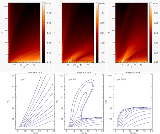
Illustration of the effect of resistivity on the density in the outflow. Top panels: in the left-hand panel, the quasi-stationary state solutions in the ideal-MHD case are shown, and in the middle and right-hand panels, solutions with large and very large resistivity, η = 10 and 100 are shown. Solutions with small resistivity are very similar to the ideal-MHD solution. Definitions of colours and lines are the same as in Fig. 1. The obtained outflow for large and very large resistivity is supersonic in the entire domain, so that the slow magnetosonic surface is not present in those cases. Bottom panels: magnetic flux isocontour lines with the above resistivities, η = 0, 10, 100 in the left, middle and right-hand panels, respectively. Contours are parallel to the poloidal magnetic field lines. With a small η, magnetic flux isocontour lines are of the same geometry as for the ideal-MHD case. We obtain three different geometries of solutions for small, large and very large resistivity. The topology of the magnetic field lines for corresponding values of resistivity is always similar to one of the three modes shown.

Open in new tabDownload slide

Figure 4.

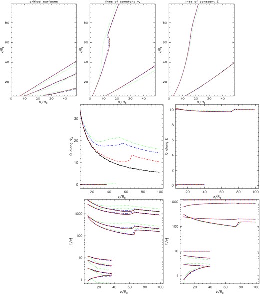
Illustration of the effect of small physical resistivity on the alignment of MHD integrals and magnetic flux surfaces. In the top-left panel, we show critical surfaces in the outflow with the resistivities η = 0, 0.01, 1 and 1.5 shown in solid (black), dashed (red), dot–dashed (blue) and dotted (green) lines, respectively. The last value is shown to illustrate the difference in comparison with solutions above the critical value of η_c = 1.0. The fast magnetosonic, Alfvén and slow magnetosonic critical surfaces are positioned from higher to lower positions in the box, respectively. In the top-middle and top-right panels, the shapes of two different poloidal magnetic field lines and energy integral isocontour lines are shown along which we compute quantities shown in the panels in the rows below (shown with the same line type and colour as in the plot of critical surfaces). As an example of the MHD-integrals, in the middle panels we show the entropy Q along those lines, normalized to its value at large distance. In the bottom panels, we show a split-down of the energy contributions along the same two lines. In both panels, the upper set of curves corresponds to the inner flux line, and the lower set of curves to the outer flux line. The colour code of the lines is for the resistivities as above. The different line types now represent energy E (solid), kinetic energy (dotted), enthalpy (dot–dashed) and Poynting flux energy (dashed). The gravitational energy is not shown as it is orders of magnitude smaller.

Open in new tabDownload slide

Figure 5.

Illustration of the effect of small, large and very large physical resistivity on the magnetic field lines and alignment of MHD integrals and magnetic flux surfaces. In the top panels, the shapes of magnetic flux isocontour lines (which are parallel to the poloidal magnetic field lines) in a quasi-stationary state in simulations with η = 0.5, 2.5, 100 in the left, middle and right-hand panels, respectively, are shown. In the middle and bottom panels, the left-hand panels show different poloidal magnetic field and energy integral isocontour lines along which quantities in the panels to their right are computed, for each resistivity. Legend of the figures is the same as in Fig. 4.

Open in new tabDownload slide

5 RESULTS WITH LARGE AND VERY LARGE RESISTIVITY

With resistivities approaching η = 1, the geometry of the solutions for the magnetic field lines starts to change. The value of η = 1 is a critical value for this change, as it is where the smooth trend described in the previous subsection no longer applies in the whole box, because of the changed geometry. The typical solution in the second mode of geometry for a radially self-similar setup is shown in the middle panels of Fig. 3. The magnetic field ‘bulges’ in the superfast magnetosonic portion of the flow, and is compressed towards the meridional plane at large radial distances.

With even larger resistivities, approaching η = 10, the magnetic field geometry drastically changes once again. The ‘bulge’ acquired with large resistivities is smoothed out, and only the compressed part of the field above the disc surface remains. The third mode of geometry for a radially self-similar setup is shown in the right-hand panels of Fig. 3. There is no longer any collimation of the magnetic field. This mode of the solution is stationary, it does not change further with an increase in resistivity. In Fig. 5 are compared magnetic field lines, MHD integrals and magnetic flux surfaces with small, large and very large physical resistivity. The largest value of resistivity for which our code still could run to a quasi-stationary state was of the order of a few hundreds.

Fig. 6 shows the Reynolds magnetic number in our computational box in simulations with increasing η. The profile of Rm traces the increasingly de-collimating outflow, indicating that the resistivity is directly related to the geometry of the magnetic field. In Fig. 7, we show various quantities along the slice parallel to the axis of symmetry, at half the computational box, for the full range of η considered in this work. The density does not differ much in our solutions. Poloidal velocity increases for large and very large resistivities. Rotation changes direction for very large resistivities. B_Z also changes direction for large and very large resistivities, but it is interesting that B_R changes direction only for large, but not for very large resistivities.

Figure 6.

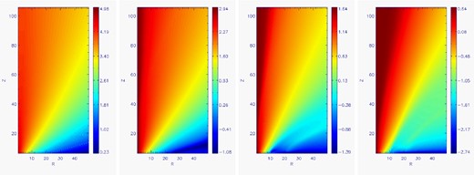
Reynolds magnetic number Rm = VΔx/η in the case of initial conditions, small, large and very large physical resistivity, shown in the logarithmic colour grading. Left- to right-hand panels show Rm for η = 0.01, 0.5, 10 and 100, respectively. The numerical resistivity, η = 0.01 is plotted at T = 0, for easier comparison of the other values of η to the solution from Vlahakis et al. (2000).

Open in new tabDownload slide

Figure 7.

Various quantities computed along the slice parallel to the symmetry axis, at half of the computational box (R = 25). In solid, dotted, dashed and dot–dashed lines for η = 0.01, 0.5, 10 and 100 are shown density, Reynolds magnetic number and R_β = μ₀RmP/B² in logarithmic scale, and R, Z and toroidal components of velocity and magnetic field, respectively.

Open in new tabDownload slide

In C08, we estimated the physical magnetic diffusivity in the astrophysical case of young stellar object with solar mass |${\cal M} \approx {\rm M}_{\odot }$| and with a characteristic distance of 0.1 au = 1.4 × 10¹⁰ m. Here, we extend it to the increased range of diffusivity. From equation (11), for the diffusivities |$\hat{\eta }=(1,10,100)$| in the code units, we obtain the physical diffusivities η = (1, 10, 100) × 6.8 × 10¹⁴ m² s⁻¹ = (1, 10, 100) × 6.8 × 10¹⁸ cm² s⁻¹, respectively.

6 SUMMARY

We obtained solutions of resistive-MHD self-similar outflows above the accretion disc for the regimes of small, large and very large resistivities. The disc is not included in the simulations, but is taken as a boundary condition.

To find the lower limit of small resistivity, we first find the level of numerical resistivity. We also verified the predicted behaviour of numerical resistivity with increasing grid resolution: it is not enough to double the grid resolution to obtain the decrease in numerical resistivity for an order of magnitude. One has to quadruple the number of grid cells. A similar procedure could be used as a standard test for resistive MHD codes.

Next, we verified the solutions from our previous work in C08, for small resistivity, since there we used a different code. We find the same trend. Since now we have a parallel code, we can investigate solutions with larger resistivities. Solutions with small, large and very large resistivities each have a different geometry, so that we can distinguish three modes of solutions.

The first mode is similar to the ideal-MHD solutions. With η > 1, there appears a ‘bulge’ in the magnetic field, which is a signature of the second mode. At even larger resistivities, with η > 10, the third mode of solutions sets in. In the third mode, the magnetic field is no longer collimated, but is pressed towards the disc. Such a solution does not change further with increasing resistivity.

MČ completed this work in the Theoretical Institute for Advanced Research in Astrophysics (TIARA) under contract funding by TIARA in the Academia Sinica and National Tsing Hua University through the Excellence Program of the NSC, Taiwan. Simulations have been initially performed during MČ stay in Athens at spring 2009, supported by the European Community's Marie Curie Actions – Human Resource and Mobility within the Jet Simulations, Experiments and Theory (JETSET) network under contract MRTN-CT-2004005592. Fruitful discussions with Ruben Krasnopolsky are acknowledged, and we thank A. Mignone for possibility to use the pluto code. MČ thanks to M. Stute for help with pluto setup, and J. Gracia for his python scripts for some of the plots.

REFERENCES