


Abstract
We present results of a study of the fast timing variability of the magnetic cataclysmic variable (mCV) EX Hya. It was previously shown that one may expect the rapid flux variability of mCVs to be smeared out at time-scales shorter than the cooling time of hot plasma in the post-shock region of the accretion curtain near the white dwarf (WD) surface. Estimates of the cooling time and the mass accretion rate, thus provide us with a tool to measure the density of the post-shock plasma and the cross-sectional area of the accretion funnel at the WD surface. We have probed the high frequencies in the aperiodic noise of one of the brightest mCV EX Hya with the help of optical telescopes, namely Southern African Large Telescope and the South African Astronomical Observatory 1.9 m telescope. We place upper limits on the plasma cooling time-scale τ < 0.3 s, on the fractional area of the accretion curtain footprint f < 1.6 × 10⁻⁴, and a lower limit on the specific mass accretion rate Ṁ/A>3 g s−1 cm−2. We show that measurements of accretion column footprints via eclipse mapping highly overestimate their areas. We deduce a value of Δr/r ≲ 10− 3 as an upper limit to the penetration depth of the accretion disc plasma at the boundary of the magnetosphere.
1 INTRODUCTION
Confining a hot (millions K) plasma in a magnetically controlled volume is not only the goal of the thermonuclear fusion reactors in terrestrial laboratories, but also is a reality near magnetic and relativistic compact objects in binary systems. It was realized quite some time ago that the strong magnetic fields of accreting white dwarfs (WDs) and neutron stars disrupt accretion flows at some distance from their surfaces to form an accretion column (or curtain) around their magnetic poles (Pringle & Rees 1972; Lamb 1974). However, very little is currently known about the geometry of these columns or curtains. It is likely that the best currently available direct measurement of the size of an accretion column footprint on a WD surface, was obtained several years ago via eclipse mapping of the polar FL Cet (O'Donoghue et al. 2006).
Indirectly, the geometry of the accretion column/curtain can be estimated from the density of the hot plasma which is heated by a standing shock wave near the WD surface. The density determines the cooling time of the plasma, thus knowing this cooling time and the total mass accretion rate in the flow we can have a handle on the accretion column/curtain geometry. Langer, Chanmugam & Shaviv (1981) showed that if the hot post-shock region is cooling only via the bremsstrahlung emission it should be thermally unstable, generating quasi-periodic oscillations (QPOs) of the shock (see also Chevalier & Imamura 1982; Imamura et al. 1996). It was expected that such oscillations should be observable as optical brightness variations (see e.g. Larsson 1995). In later studies, it was shown that there were mechanisms, like influence of cyclotron cooling, which can stabilize the post-shock region (e.g. Chanmugam, Langer & Shaviv 1985; Wu, Chanmugam & Shaviv 1994; Wu & Saxton 1999; Wu 2000; Saxton & Wu 2001); it may be for this reason that predicted QPOs are seen only in a small fraction of all magnetic cataclysmic variables (mCVs). Another possible mechanism which might make the post-shock region oscillations invisible in light curves is incoherent variations of different parts of the accretion column. If the accretion flow is not uniform, but spread over a large number of quasi-independent filaments, their individual oscillations might be not in phase with each other. Therefore, even if the hot plasma cooling time-scale is similar in these filaments, their total emission will be the sum of incoherent brightness oscillations of individual filament and will be strongly dumped (Drake et al. 2009).
More recently, it was proposed that in spite of the relative absence of QPOs in mCVs, one can still probe the cooling time of the accretion column plasma via the properties of their aperiodic variability (Semena & Revnivtsev 2012). It was proposed that aperiodic variability of the mass accretion rate in accretion columns, which, as we know from observations of accreting neutron stars, continues towards frequencies above 100 Hz (see e.g. Jernigan, Klein & Arons 2000), should not produce strong variability in the luminosity at time-scales smaller than the cooling time of plasma in the hot post-shock region. All variability at higher frequencies should be smeared out for periods less than this cooling time-scale, producing a break in the power-density spectrum of the brightness variations.
The search for such a break was done in optical light of a bright Northern hemisphere intermediate polar (IP), LS Peg (Semena et al. 2013). Choosing to study mCVs in optical light has certain advantages. The main gain is in the relative increase in the number of optical photons generated by the WD/accretion disc, due to X-ray illumination from the post-shock region. Depending on the geometry and inclination of the system, this number can far exceed that of X-ray photons reaching us directly from the post-shock region.
Unfortunately, due to the small level of aperiodic variations of light of LS Peg at high frequencies (<0.2 per cent at f > 0.1 Hz), only an upper limit (<10 s) on the cooling time-scale was obtained.
In this paper, we are furthering the search for the cooling time generated turnover frequency in the rapid variability of mCVs. Our target is one of the brightest accreting magnetic WDs in the Southern hemisphere, EX Hya.
2 EX Hya
EX Hya is one of the closest and brightest IPs, which makes it one of the best candidates for searching for cooling time features in the power-density spectra of optical flux variations in magnetic CVs. Physical parameters of the system used in this study are listed in Table 1.
Parameters of EX Hya, used in the paper.
| Parameter | Value | Reference |
|---|---|---|
| Orbital period, h | 1.63 | |
| Mass WD, MWD | 0.79 M⊙ | 1 |
| Radius WD, RWD | 0.7 × 109 cm | 1 |
| Secondary radius, R2 | 1.04 × 1010 cm | 1 |
| Inner disc radius, Rin | 1.9 × 109 cm | 2,3 |
| WD magnetic field, B | <1 MG | 4 |
| ∼ 7-8 kG | 5 | |
| Mass accretion rate, |$\skew4\dot{M}$| | 3 × 10¹⁵ g s−1 | 6 |
| Binary separation, a | 4.68 × 1010 cm | 1 |
| Binary inclination, i | 77.8° cm | 7 |
| Luminosity, Lx | 2.6 × 1032 erg s−1 | 1 |
The mass accretion rate on to WD in this binary system demonstrates stochastic variability, which we see through variations of its X-ray and optical flux (e.g. Watson & Rayner 1974; Revnivtsev et al. 2011). The accretion flow in this binary occurs via an accretion disc, disrupted at a distance of approximately 2 × 109 cm (Siegel et al. 1989; Hellier 1997; Revnivtsev et al. 2011). Assuming that this disruption is due to influence of a dipole magnetic field of the WD, we can obtain an approximate estimate of its magnetic field from a simple formula of magnetospheric radius of accreting compact object (e.g. Pringle & Rees 1972): |$R_{\rm in}\sim \mu ^{4/7} ({GM}_{\rm WD})^{-1/7} \skew4\dot{M}^{-2/7}$|, where μ is the magnetic moment of the compact object. Substituting parameters from Table 1, we obtain μ ∼ 2.5 × 1030 G cm−3, which corresponds to magnetic field strength on WD surface B ∼ 7 kG. This value is in agreement with upper limit B < 1 MG, inferred from spectroscopic observations of the system in infrared spectral band (Harrison et al. 2007). Such low-magnetic field of the WD means that the cyclotron cooling mechanism is not important for the dynamics of the post-shock region of the accretion column, that the dominant cooling is the optically thin plasma bremsstrahlung emission (see e.g. Lamb & Masters 1979; Chanmugam et al. 1985), and that electrons and ions in the accretion column/curtain has the same temperatures (e.g. Imamura et al. 1987).
We used numerical integration techniques similar to Wu et al. (1994) in order to estimate the plasma cooling time, and thus the accretion channel cross-section. The WD mass and radius were fixed, while the accretion channel cross-section was varied to obtain the expected cooling time. To check different possibilities, we made use of the flat channel geometry of Wu et al. (1994) and the dipole channel geometry of Canalle et al. (2005); see equations 37 and 38. In both cases, gravity of the WD and bremsstrahlung cooling were taken into account.
We assume that the field lines of the magnetic dipole, which form the boundary of the accretion curtain, start at the inner edge of the accretion disc Rin, and that matter from the surrounding area then settles on to these field lines. We also assume, for simplicity, that the magnetic dipole and the spin axis of the WD are co-aligned (this is of course an oversimplification but sufficient for our present estimates). We can then put an upper limit on the accretion curtain cross-sectional area, |$A < \pi R_{{\rm c}}^2 = \pi R_{\rm WD}^3/ R_{\rm in} \sim 5.6\times 10^{17}$| cm2, where RWD is the WD radius and Rin the inner radius of the disc.
For cross-sectional area A = 2.8 × 1017 cm2, the corresponding cooling time is τ ≈ 15 s, while for cross-sectional area |$A = 0.01 \ 4 \pi R_{\rm WD}^2 = 6 \times 10^{16}$| cm2 the cooling time τ ≈ 6 s. In the case of pure bremsstrahlung cooling, we can therefore expect that source flux variability should be smeared out at frequencies above >0.05–0.5 Hz.
3 APERIODIC VARIATIONS OF THE EX Hya OPTICAL LIGHT
Matter, which impacts the WD surface in accretion columns/curtains is heated up to high temperatures and emits X-ray radiation. The X-ray flux of even the brightest accreting magnetic WDs is relatively small (of the order of 10−3 photons cm2 s−1), which complicates any study of their fast timing variability. However, part of this X-ray emission is intercepted by the underlying WD surface and the accretion disc, and re-emitted in optical/UV energy range with much larger photon fluxes (Beuermann et al. 2004; Revnivtsev et al. 2011). Any variations in X-ray luminosity of the post-shock region should therefore also be visible in optical light variations. These optical light variations look like flicker noise, often observed in accreting WD binaries (see e.g. Bruch 1992; Baptista & Bortoletto 2004). The goal of our paper is to use the optical light flickering to understand properties of the post-shock region.
Since we analyse the optical emission of the binary instead of its X-ray emission, we should take into account some modification of the emerging flux variability.
3.1 Power-density spectrum
There are two main reasons for the power-density spectrum of the optical flux variability to change: (a) smearing of variability due to finite light crossing time of the reprocessor and (b) smearing, caused by a finite time, required for the reprocessor (inner part of the accretion disc of the WD surface) to absorb and re-emit incoming X-rays. The latter effect was considered, e.g. by Cominsky, London & Klein (1987), where it was shown that the reprocessing time-scale for parameters relevant for our study is not larger than ∼1 s (see also Hummer & Seaton 1963; O'Brien et al. 2002).
In order to model the effect of smearing due to light crossing time of the reprocessing region, we have calculated the transfer function of the reprocessor in two scenarios. First, we assumed that the reprocessor is an annulus with the inner disc radius Rin = 1.9 × 109 cm and (1) the outer radius Rout = 3 × 109 cm, or (2) the outer radius 1010 cm. Values of the outer radii of the reprocessing disc annulus (which is the most important parameter of the smearing kernel) were adopted using the following arguments. In the work of Siegel et al. (1989), it was shown that the optically bright region is located at a distance ∼1.5 × 109 cm from the WD. The maximal outer radius of the optically bright region can be estimated also from the length of the optical eclipse: adopting the orbital inclination of the binary i = 77| $_{.}^{\circ}$|8 (Hellier et al. 1987) and the size of the secondary R2 ∼ 1.04 × 1010 cm (Beuermann & Reinsch 2008) the length of the eclipsing chord of the secondary can be estimated as ≲ 5 × 109 cm. The shape of the eclipse shows that the emitting region should have a similar size.
In the model, the illuminating X-ray source is raised at 0.6 × 109 cm above the plane of the disc, the disc has the shape H ∝ R9/8 (Shakura & Sunyaev (1973)).
The power spectrum of simulated flux variability of an accreting magnetic WD, modified by disc reflection (along with power-density spectrum of intrinsic variability) are shown in Fig. 1. It is seen that the effect of smearing in any case is important only at Fourier frequencies above few Hz.
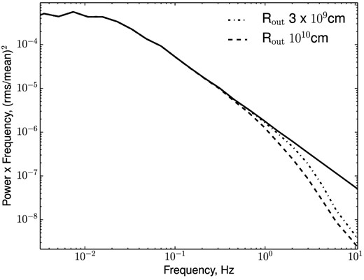
Power spectrum of intrinsic variability of the source and its modifications due to smearing caused by reflection from disc. We present results of two models, where the reprocessor is an annulus with inner radius Rin = 1.9 × 109 cm, and the outer radius rout = 3 × 109 cm (dotted curve) and rout = 1010 cm (dashed curve).
4 OBSERVATIONS
In order to study properties of aperiodic variability of EX Hya in the optical, we have used a set of observations from telescopes at the South African Astronomical Observatory (SAAO), including Southern African Large Telescope (SALT). Table 2 contains a list of observations.
Observations of EX Hya on telescopes of SAAO, used in this work.
| Date | Time resolution, s | Duration, s | ut start time | Device | Filter |
|---|---|---|---|---|---|
| 15.04.2010 | 1.0 | 5100 | 19:37 | HIPPO | R |
| 17.04.2010 | 1.0 | 4700 | 23:21 | HIPPO | R |
| 18.04.2010 | 1.0 | 4600 | 19:43 | HIPPO | R |
| 29.03.2012 | 0.067 | 3239 | 02:52 | SHOC | White light |
| 02.04.2012 | 0.067 | 3500 | 03:00 | SHOC | R |
| 07.05.2012 | 0.1 | 2500 | 23:00 | SALTICAM | CLR-S1 |
| 07.02.2013 | 0.16 | 3760 | 23:50 | SHOC | White light |
| 07.04.2013 | 0.1 | 1064 | 01:35 | BVIT | White light |
| 02.08.2013 | 0.16 | 5118 | 00:53 | SHOC | White light |
| 15.06.2013 | 0.057 | 7485 | 17:08 | SHOC | R |
| 17.06.2013 | 0.032 | 7106 | 16:43 | SHOC | R |
| 18.06.2013 | 0.032 | 3923 | 16:51 | SHOC | R |
| 18.06.2013 | 0.032 | 4102 | 18:03 | SHOC | B |
4.1 SALT/SALTICAM
We obtained approximately 2.5 ks of fast photometry on the SALT using SALTICAM with a Sloan r′ filter on 2012 May 7, from 23:00 UTC to 24:00. Observations were performed in Slot Mode, with 6 × 6 binning, providing 0.1 s time resolution (O'Donoghue et al. 2006). Slot Mode employs the following readout algorithm: a slot in front of the CCD leaves open only 144 unbinned rows (approximately 20 arcsec on the sky) of the CCD, just above the frame transfer boundary. During one exposure time, the signal is accumulated on the open part of the CCD. At the end of the exposure, these 144 rows rapidly (∼14 ms) move over the frame transfer boundary. These images then migrate to the readout register in a stepwise manner. Start times of two consequent exposures differ by 104 ms (i.e. time resolution of our data). The SALTICAM readout algorithm has some features which affect data analysis. The time series have a time gap every 6.2 s, lasting between ∼0.1 and ∼0.6 s. Such periodic time gaps should be carefully taken into account in all studies of source fluxes aperiodic variability power spectra. Therefore, in our analysis, we have split Fourier frequency range into two intervals, above and below 1/6.2 Hz. The power spectrum at Fourier frequencies above 1/6.2 Hz was obtained from evenly sampled data between gaps. The power spectrum at Fourier frequencies below 0.08 Hz was obtained from the light curve binned into 6.2 s time bins.
A typical image of the target star with a comparison star is shown in Fig. 2. Our reduction algorithm is similar to that of standard pysalt slottools package (Crawford et al. 2010), but with some differences. Photometric measurements of target and comparison stars were performed with fixed apertures around best-fitting centroids of the two stars, determined in each frame. We assume that the background consists of a constant value and the vertical trail of the star, created by light from the star trailing during frame transfer from the image to the storage area of the CCD (the shutter remains open in Slot Mode). Typical selection regions are shown in Fig. 3. The background value was measured as a median outside 3.75 arcsec aperture around stars and within 8.33 arcsec square, see Fig. 3. Our measurements show that the vertical trail contains about 4 per cent of signal in 4.5 pixel star aperture, thus it should be carefully taken into account. We have adopted the following approach: we measured the mean shape of the trail profile over the areas, shown in Fig. 3. This profile was extracted from each frame row.
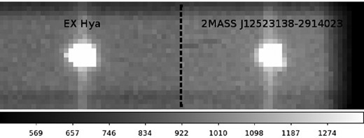
Typical image frame with EX Hya (left object) and a comparison star (right object) collected over 0.1 s. The grey-scale shows the number of counts per pixel.
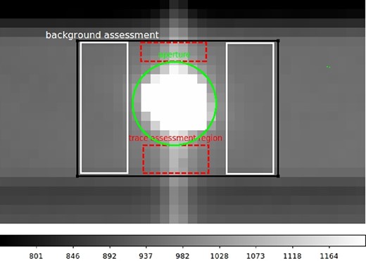
Illustration of apertures, used for photometric measurement of stars. Circular apertures with radius 4.5 pixels were used to collect counts from a star. Rectangular regions to the left and to the right from the star were used to estimate the background level. Dashed rectangles were used to estimate the shape of the trail.
As the first step of correction for the atmospheric influence, we have divided the flux of the target star by the flux of a comparison star 2MASS J12523138−2914023 (differential photometry). Due to poor weather conditions, a substantial fraction (approximately 50 per cent) of our observations are not acceptable for the subsequent analysis. We have determined this from the light curve of the comparison star. The raw count rate of the comparison star is shown in Fig. 4, where excluded time intervals are shown by shaded areas. The remaining data were split into evenly sampled time intervals, each 6 s long. The exposure time of our data set filtered for the bad weather conditions is 1340 s. Example of the source light curve is shown in Fig. 5. It is clearly seen that aperiodic variability of the source flux exists down to at least 1 s time-scale.
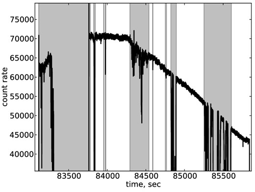
Count rate of a comparison star during our observation. Due to poor weather condition some parts of our observations were affected by clouds. We have excluded time periods, shown by shaded areas from the subsequent analysis.
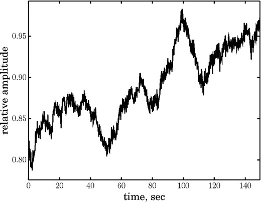
A section of a light curve of EX Hya, which demonstrate aperiodic variations of the light down to at least 1 s time-scale.
Numerous gaps in SALTICAM data set (typically every 6 s, are due to features in the readout sequence) preclude usage of simple Fourier transforms to obtain power spectrum of the source variability. Thus, we have obtained the power spectrum in two steps, at frequencies above 1/6 Hz and below 1/13 Hz.
Seeing as the power spectrum at Fourier frequencies above 1/6 Hz has a steep slope of around −2 (P(f ) ∝ f−2) (see e.g. Revnivtsev et al. 2011), the simple rectangular window function can produce artificial power at all relevant frequencies. In order to reduce this effect, we have multiplied data in each time interval by a Hann window function before calculation of the power spectra. This multiplication was done for all data sets from all instruments.
The resulting power-density spectrum of EX Hya (in relative units (rms mean)−2 Hz−1, see e.g. Miyamoto et al. 1991) obtained by averaging over all power spectra, calculated for every time interval, is presented in Fig. 6. Uncertainty in the power value at any particular frequency interval was calculated from dispersion of all values of power, which fall into this interval. Such an approach provides us the most robust estimate of the uncertainty. This automatically includes all measurement errors and all uncertainties connected with intrinsic red noise in the source flux variations. This approach was also applied to all data sets, which we describe below.
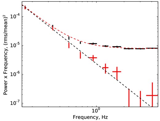
Power spectrum of EX Hya, obtained by averaging over power spectra of all 6 s time intervals. The upper set of crosses show raw power-density spectrum, which contains contribution from Poisson noise of photon counts. The lower set of crosses shows intrinsic power-density spectrum of EX Hya. The dashed line shows a power law with slope α = 2.5.
The periodogram clearly contains the intrinsic source variability at frequencies below 1 Hz, and is dominated by noise at higher Fourier frequencies. The dominant contribution to the noise component is Poisson noise of photon counts, which we see as a constant value in units (rms mean)−2 Hz−1 (at the level approximately ∼8 × 10⁻⁶ (rms mean)−2 Hz−1).
Atmospheric turbulence along the light path adds a band-limited noise (scintillation) to power spectra of optical objects (see e.g. Dravins et al. 1998; Revnivtsev et al. 2012). It is known that the amplitude of this noise is smaller for larger telescopes (Dravins et al. 1998) and in the case of SALT/SALTICAM observations we do not detect it. In order to estimate an upper limit to the atmospheric scintillation component, we fit the power spectrum using model with additional component Patm = A(1 + (f/f0)2)−0.3, f0 ∼ 0.8 Hz. The upper limit on contribution of atmospheric scintillations at 1 Hz is about ∼5 × 10⁻⁶ (rms mean)−2 Hz−1.
4.2 SALT/BVIT
BVIT – The Berkeley Visible Image Tube is a photon counter with quantum efficiency about ∼15 per cent and angular resolution approximately 0.3 arcsec, mounted on SALT (Buckley et al. 2010; Welsh et al. 2012). BVIT makes observations in the format of 25 ns time resolution event list in a circular, 1.6-arcmin diameter field of view. The target, the background and the comparison star apertures were selected during data processing. We have binned all count rates into 0.01 and 0.1 s time resolution bins. All BVIT data processing made use of the BVIT data standard processing tools (Welsh et al. 2012).
The mean BVIT count rate of EX Hya with background is 5.9 kcps, while the mean background count rate is 0.9 kcps. The background rate is not constant and contains shot noise variations as well as long-term trends. Point-to-point subtraction of the background curve from the count rates of EX Hya will increase the shot noise of the resulting light curve, therefore it is better to subtract a model of the background count rate variations. Analysis of the time variable background count rate shows that a third-order polynomial fit describes it well.
The resulting power spectra of EX Hya from BVIT data (original and shot-noise-subtracted) are presented in Fig. 7.
Power spectrum of EX Hya light curve received by SALT/BVIT. The dashed line shows a power law with slope α = 2.48.
4.3 1.9 m/SHOC
SHOC (Sutherland High-speed Optical Camera) consists of an Andor iXon 888 CCD camera (similar to that used by our group on RTT150 telescope; Revnivtsev et al. 2012) and auxiliary systems (Coppejans et al. 2013). For our observations, SHOC was mounted on the SAAO 1.9 m telescope. SHOC was used in both conventional and electron-multiplying modes, with binning optimized to the seeing conditions on each night.
Instrumental magnitudes for EX Hya were extracted using iraf daophot (Stetson 1987) tasks for different apertures. Aperture-corrected photometry was then performed by using the iraf MKAPFILE task (Davis & Gigoux 1993), extracting the magnitudes for the smallest apertures that maximize the signal to noise and ignoring data points with errors larger than 0.1 mag. The data were then filtered to eliminate outliers, which were detected using a simple algorithm which marks as an outlier any point outside of 5σ from the median of five neighbouring points. The sigma parameter for this filter was the standard deviation of 100 points preceding the given one, which were initially detrended by making a linear fit.
Power spectra of EX Hya light curve, obtained in one of the 1.9 m/SHOC observations. Upper set of points shows raw power spectrum, which contains photon counting noise and noise of atmospheric scintillations. Lower set of points shows EX Hya power spectrum with subtracted noise components. The dashed line shows a power law with slope α = 2.48.
4.4 1.9 m/HIPPO
For completeness, we also used light curves of EX Hya obtained on the SAAO 1.9 m telescope using the HIPPO photopolarimeter (Potter et al. 2008), presented in work of Revnivtsev et al. (2011). HIPPO is a two-channel instrument capable of simultaneous dual filtered photopolarimetry. We present results of light curves collected in one filter (R). Data reduction was done as outlined in Potter et al. (2010) and binned to 1 s time resolution.
5 RESULTS
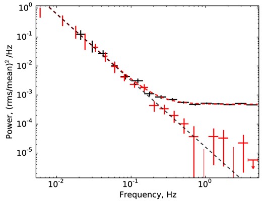
Power spectra from observations obtained at the SAAO with SALT/SALTICAM, SALT/BVIT, SAAO 1.9 m/SHOC and SAAO 1.9 m/HIPPO (shown in Fig. 9) were analysed at frequencies above 0.05 Hz. All SHOC observations were split into eight parts which have approximately similar levels of atmospheric oscillations and Poisson noise. SALTICAM data were split into two parts with similar levels of Poisson noise.
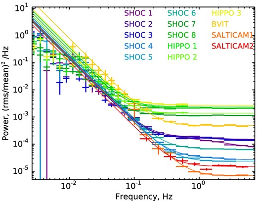
Power spectra of EX Hya, obtained during different observations with different instruments along with their best-fitting models (solid curves).
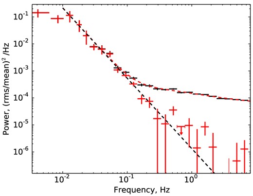
Power spectra of all separate light-curve segments, renormalized to the average normalization, are shown in Fig. 10. For this plot, we have subtracted fitted contributions of all noise components.
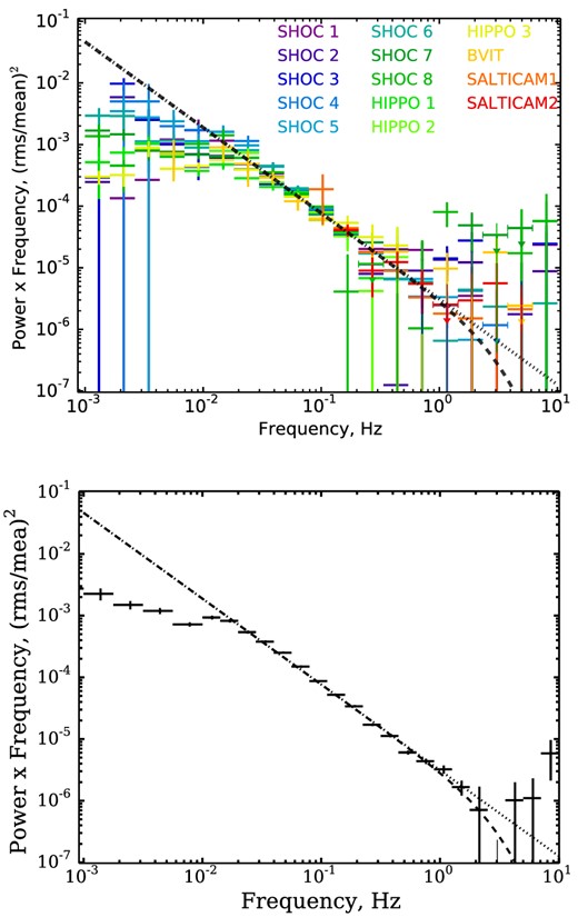
Broad-band power-density spectrum of aperiodic variations of optical light of EX Hya, obtained by different instruments (upper panel) and averaged over all presented measurements (lower panel). Dotted line shows a power law with the slope α = 2.4. Dashed curve (with rollover at high frequencies) shows the same power law with a break at fbreak = 4.4 Hz.
In order to present the frequency binned power spectrum of EX Hya averaged over all analysed data sets, we also used maximum likelihood technique. In this case, the mean value of the power in any individual frequency bin was estimated by maximizing the likelihood function assuming that the model function is constant within this frequency bin. The confidence interval on the mean value of the power in this frequency bin was obtained adopting intervals of power values, where Δlog L = 0.5.
The power spectrum obtained after averaging over all available data sets is presented in Fig. 10. The power spectrum does not show any evidence of QPOs, with a typical upper limits of 0.3 per cent. The best-fitting approximation of obtained data points give the value of the slope α = −2.40 ± 0.05, the 2σ lower limit on the break frequency fbreak > 3.5 Hz. The quality of the fit can be accessed via calculation of χ2 values on binned power spectra. For the PDS averaged over all data set, the χ2 = 13.5 for 12 degrees of freedom.
5.1 Area of accretion curtain footprints
From this equation, the area of both curtains (accretion is going on to two poles) is A < 1015 cm2 and the specific mass flux is about |$\skew4\dot{M}/A>3$| g s−1 cm−2. This simple approach underestimates the cross-sectional area due to the underestimating of the cooling rate in the hot zone. A more accurate estimate of the cross-sectional area A can be derived by taking into account the profiles of the temperature, velocity and density in static hydrodynamic flow through the accretion column (Wu et al. 1994). The effect of gravity in the column and geometrical compression, which can play significant role in the case of tall accretion columns, also should be taken into account (Canalle et al. 2005).
We use the Canalle et al. (2005) one-dimensional equations of the stationary flow (equation 37, 38 in that paper). We assume that accreting matter flows from the inner disc radius along the magnetic field lines through the geometrically thin curtains to the two areas on the opposite sides of the WD. Each curtain collects half of the accreted matter. Adopting the system parameters from Table 1, the minimum possible cooling mechanism (|$\Lambda _{\rm bremss} \sim 1.4 \times 10^{-27} n^2 \sqrt{T}$|) and cooling time (τ < 0.3 s), we get for a single curtain footprint a surface area A < 1015 cm2 and a mass accretion rate of |$\skew4\dot{M}/A> 3$| g s−1 cm−2. Small area of the accretion curtain footprint was also estimated from X-ray spectra of EX Hya. Evans & Hellier (2007) interpreted a soft blackbody component seen in X-ray spectrum of EX Hya as an area of WD surface, heated by the X-ray emitting accretion column, and thus obtained an estimates of its area A ≈ 1014 cm2.
The value of the specific mass accretion rate, which we estimate here, is very important. Usually, this parameter is an ingredient of all models of X-ray spectra of IPs (see e.g. Cropper, Ramsay & Wu 1998; Suleimanov, Revnivtsev & Ritter 2005; Yuasa et al. 2010). However, it is highly degenerate for observational data with limited energy resolution (i.e. if there are no abilities to make detailed emission line diagnostics). This degeneracy usually leads to adopting some fiducial parameters of the specific mass accretion rates. Here, we are able to put physically important constraints on this parameter.
It should be noted that with the obtained parameters the accretion curtains might become optically thick with respect to Compton scattering in the vertical direction (i.e. along the direction of mass flow). This might have an influence on the spectral shape of the emission of the post-shock region (see e.g. Suleimanov et al. 2008) and on its angular dependence, producing pulsed emission.
The length of the accretion curtain can be estimated from eclipse mapping. In particular, Mukai et al. (1998) showed that the egress and ingress of eclipses of X-ray emitting regions last about 21 s, which can be recalculated into a maximal spatial size of the X-ray emitting accretion curtain near the WD surface of l ∼ 109 cm. For this length, the accretion curtain thickness should then be ≲ 106 cm.
It is important to emphasize here that the area of the accretion curtain footprints, which we measure here with the cooling time method, is significantly smaller than that, estimated from eclipse mapping (see e.g. Hellier 1997; O'Donoghue et al. 2006). However, there are no contradictions here because the eclipse mapping essentially determines the maximal spatial size of the accretion curtain and not its area (in a sense it determines the upper limit on the area of the column). As an illustration of this difference, in Fig. 11 we show a schematic of the accretion curtain footprint along with limits of its sizes from the eclipse mapping.
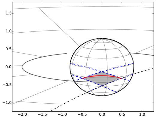
Schematic view of the accretion curtain geometry. The scheme illustrates that the area of the rhombus, which limits the size of the accretion curtain footprint and which is determined from the eclipse mapping, can be significantly larger than the real area of the accretion curtain – thin stripe within the rhombus. Part of big dashed circle (at the lower-right corner of the plot) denotes the secondary at the position immediately after the egress of X-ray eclipse.
The deduced parameters of the accretion curtains imply that the plasma density in the curtains increase from n ∼ 1016 cm−3 to n ∼ 1017 cm−3 in its luminous part. We postulate that this range of hot plasma (T ∼ (50-200) × 106 K) densities can be probed with iron emission lines diagnostics (see e.g. Hayashi & Ishida 2014) if high-energy resolution spectra of the curtains will be available from future calorimeter experiments aboard, e.g. satellites Astro-H (Takahashi et al. 2010) or Athena+ (den Herder et al. 2012).
5.2 Matter coupling region at the magnetospheric boundary
Assuming that the matter flows strictly along the magnetic field lines of the WD dipole, we can relate the thickness of the accretion curtain at the WD surface with Δr, the radial extent of the plasma–magnetosphere coupling region at the inner edge of the accretion disc (see e.g. Rosen 1992). Assuming that the magnetic dipole and the accretion disc rotation axis are coaligned (which is a reasonable assumption at the current level of accuracy of our estimates), the cross-sectional area of one curtain corresponds to a depth Δr/Rin < 10−3. Note that the size of this coupling region is significantly smaller than that assumed in many works on magnetic accretion (see e.g. Basko & Sunyaev 1976; Ghosh & Lamb 1978; Hameury, King & Lasota 1986; Buckley & Tuohy 1989; Rosen 1992; Kim & Beuermann 1995; Ferrario 1996).We can try to compare this number with some physical estimates of the plasma layer thickness on top of the magnetosphere (see also discussion of this topic in Ghosh & Lamb 1978, 1979; Ichimaru 1978; Anzer & Boerner 1980; Spruit & Taam 1990; Campbell 1992, 2010; Lovelace, Romanova & Bisnovatyi-Kogan 1995).
It is commonly accepted that matter at the inner part of the accretion disc starts to flow along magnetic field lines when the (central object) magnetic field energy density exceeds the matter pressure. The flow along the magnetic field lines very rapidly becomes supersonic, but the motion of plasma across the field lines is strongly suppressed, and thus is significantly subsonic in this direction.
Thus, we propose that the thickness of the plasma flow in the magnetosphere is set by its dynamical settling at the magnetospheric boundary. Different works, adopting reasonable assumptions about the accretion disc magnetic diffusivity, give estimates of Δr ≲ cs/ωK (see e.g. Campbell 1992; Shu et al. 1994; Lovelace et al. 1995; Campbell 2010), which is in general agreement with results of direct numerical simulations (e.g. Long, Romanova & Lovelace 2005; Romanova et al. 2014).
In the case of EX Hya, the size of the magnetosphere (∼3–5 RWD; Siegel et al. 1989; Hellier 1997; Revnivtsev et al. 2011) is smaller than the corotation radius (∼50RWD). This means that there should be a strong shear (vm/vK ∼ 0.01) between the magnetospheric boundary and the accretion disc plasma. This shear should significantly suppress the interchange (Rayleigh–Taylor) instability, often assumed to be operating in the case of accretion on slow magnetic rotators (see e.g. Arons & Lea 1976; Romanova, Kulkarni & Lovelace 2008). Part of the excess rotational energy (which is not transferred to the rotational energy of the WD) should result in some additional heating of the innermost part of the accretion disc. This additional energy release cannot heat the matter to X-ray temperatures, because eclipse mapping of EX Hya showed that the X-ray emitting region in this system is confined to the WD surface (e.g. Mukai et al. 1998). Thus, the effective temperature at the innermost edge of the disc should be less than < 2–3 eV ( < 20-30 × 103 K; Mauche 1999).
Adopting the other parameters of our binary, we can conclude that the thickness of the inner disc should be H/R ≲ 5 × 10− 3 − 10− 2. Thus, the size of the coupling region at the boundary of the magnetosphere is ΔR/R ≲ H/R ≲ 5 × 10− 3, which is in agreement with our findings.
5.3 Impact for neutron stars
Accretion flow on to magnetic neutron stars should form magnetosphere–disc interaction regions quite similar to those of accreting magnetic WDs. The size of the WD magnetosphere in EX Hya is ∼1.9 × 109 cm. This is close to size of magnetosphere of well-known magnetic neutron star accretor EXO 2030+375 in its faint state (e.g. Reig & Coe 1998). An estimate of the magnetic moment μ of the WD in EX Hya ∼2.5 × 1030 G cm−3 is close to that of the neutron star in EXO 2030+375 ∼ (2-10) × 1030 G cm−3 (e.g. Klochkov et al. 2007), thus, the magnetic field strength at the boundary of the accretion disc in these systems are of the same order. The mass accretion rate in faint state of EXO 2030+375 (with Lx ∼ 1036 erg s−1) is only few times higher than that in EX Hya. The only difference is the higher level of illuminating X-ray flux from accreting neutron star in EXO 2030+375, which might lead to some additional heating of the innermost parts of the accretion disc.
6 SUMMARY
In this work, we are trying to determine the area of accretion curtain footprints on the surface of the accreting magnetic WD in the binary system EX Hya. Our approach is based on measurements of the hot post-shock plasma cooling time. The plasma in the accretion curtains, which is heated in the standing shock above the WD surface, cools on a time-scale which is determined by its density. All variations in the mass accretion rate at the WD surface at time-scales smaller than this (and we know that such fast mass flux variations do exist in accreting neutron star binaries) should be effectively smeared out in the luminosity variations. Knowing the values of the total mass accretion rate at the WD surface, the hot plasma temperature and cooling time allows us to make an estimate of the accretion curtain footprint area.
We have attempted to measure the smearing time-scale with the help of fast timing observations of one of the brightest IPs, EX Hya, with optical telescopes at the SAAO. The principle is based on the fact that a significant part of optical emission from EX Hya originates as reprocessed X-rays in the post-shock region of the WD accretion curtains.
We have used a set of nine observations on different telescopes and produced a power spectrum of EX Hya in Fourier frequency interval ∼ 10− 3-5 Hz. Unfortunately, the total exposure time of our best quality highest time resolution data set, from SALT, is only 1340 s. However, the quality of the SALT data shows that we can obtain good quality power spectra at high frequencies for estimating cooling time-scales.
Our current findings can be summarized as follows.
Power spectrum of EX Hya at Fourier frequencies above 0.05 Hz can be adequately described by a power law P(f ) ∝ f−α with a slope α ∼ 2.4.
With the available data set, we place an upper limit on the hot plasma cooling time-scale on the order of 0.3–0.5 s.
This hot plasma cooling time puts an upper limit on the area of the accretion curtain footprints on WD surface of EX Hya, A < 1015 cm2, and a lower limit on the mass flux of |$\skew4\dot{M}/A>3$| g s−1 cm−2.
Our findings imply that the electron scattering (Compton) optical depth of the hot post-shock plasma in the vertical direction might be close to, or more, than unity, which would lead to some distortions of the emergent energy spectrum and its angular distribution.
We deduce that the density of hot plasma in accretion curtains should be in the range n ∼ 1016−17 cm−3. This range of densities can be probed with X-ray iron emission line diagnostics with future high-energy resolution X-ray calorimeters.
We conclude that our estimate of the accretion curtain footprint area is significantly smaller than that deduced from the eclipse mapping technique. This happens because eclipse mapping effectively determines the maximum geometrical sizes of curtains and thus their maximal possible areas within those size limits.
From the thickness of the accretion curtain at the WD surface, we determine that the extent of the coupling region at the boundary of WD magnetosphere in EX Hya to be Δr/r < 10−3, which is in line with presently available theoretical and numerical estimates of this value.
If we assume that coupling region at the boundary of magnetosphere has a similar value Δr/r < 10−3 in the case of accreting neutron stars, then we can estimate the fractional area of the neutron star accretion column |$A/4\pi r_{\rm NS}^2<10^{-5}$|. Such a small fractional area of the column should result in very high mass flux, and thus should have strong influence on the column structure.
This material is based upon work supported financially by the National Research Foundation. Any opinions, findings and conclusions or recommendations expressed in this material are those of the author(s), and therefore the NRF does not accept any liability in regard to thereto. This work was partially supported by grants of Presidium of Russian Academy of Sciences P21, programme OFN16 of RAS, by grants NSH-5603.2012.2, RFBR-13-02-00741, RFBR-14-02-93965 as well as grants from the South African National Research Foundation (NRF) Professional Development Programme (PDP).
Some of the observations reported in this paper were obtained with the SALT.
