


Abstract
We present emission-line flux distributions and ratios for the inner ≈200 pc of the narrow-line region (NLR) of the Seyfert 2 galaxy NGC 1068, using observations obtained with the Gemini Near-infrared Integral Field Spectrograph (NIFS) in the J, H and K bands at a spatial resolution of ≈10 pc and spectral resolution of ≈5300. The molecular gas emission – traced by the K-band H2 emission lines – outlines an off-centred circumnuclear ring with a radius of ≈100 pc showing thermal excitation. The ionized gas emission lines show flux distributions mostly outlining the previously known [O iii] λ5007 ionization bi-cone. But while the flux distributions in the H i and He ii emission lines are very similar to that observed in [O iii], the flux distribution in the [Fe ii] emission lines is more extended and broader than a cone close to the nucleus, showing a ‘double bowl’ or ‘hourglass’ structure. This difference is attributed to the fact that the [Fe ii] emission, besides coming from the fully ionized region, comes also from the more extended partially ionized regions, in gas excited mainly by X-rays from the active galactic nucleus. A contribution to the [Fe ii] emission from shocks along the bi-cone axis to north-east and south-west of the nucleus is also supported by the enhancement of the [Fe ii](1.2570 μm)/[P ii](1.1885 μm) and [Fe ii](1.2570 μm)/Paβ emission-line ratios at these locations and is attributed to the interaction of the radio jet with the NLR. The mass of ionized gas in the inner 200 pc of NGC 1068 is MH ii ≈ 2.2 × 10⁴M⊙, while the mass of the H2 emitting gas is only MH2 ≈ 29 M⊙. Taking into account the dominant contribution of the cold molecular gas, we obtain an estimate of the total molecular gas mass of Mcold ≈ 2 × 10⁷ M⊙.
1 INTRODUCTION
NGC 1068 is the brightest and most studied Seyfert 2 galaxy, being considered the prototype of this class, after the discovery of a Seyfert 1 spectrum in polarized light (Antonucci & Miller 1985), what led to the proposition of the Unified Model for active galactic nuclei (hereafter AGN; Antonucci 1993). Hundreds of papers have been published on its properties, obtained from data spanning the electromagnetic spectrum from X-rays to radio wavelengths. The mass of the super-massive black hole in the nucleus of NGC 1068 is M• = 8.6 ± 0.6 × 10⁶ M⊙ as obtained from the Keplerian motions of water maser clouds in a disc surrounding the nucleus (Lodato & Bertin 2003; Kormendy, Bender & Cornell 2011).
Optical narrow-band images of the narrow-line Region (NLR), obtained with ground-based telescopes as well as with the Hubble Space Telescope (HST), revealed an approximately cone-shaped structure with an opening angle of ≈65° and oriented along the position angle (hereafter PA) 15° (e.g. Pogge 1988; Evans et al. 1991; Macchetto et al. 1994). The HST narrow-band [O iii] λ5007 Å image of the NLR shows several knots and filaments of enhanced emission (e.g. Evans et al. 1991; Macchetto et al. 1994; Cecil et al. 2002). In radio wavelengths, NGC 1068 shows a kiloparsec-scale radio jet, with the brightest structure being a compact bent nuclear radio jet, less than 1 arcsec in extent (Gallimore et al. 1996, and references therein). Although the jet leaves the nucleus at PA ≈ 15°, the jet is deflected at the so-called cloud C1 to PA ≈ 30°. Gallimore, Baum & O'Dea (2004) has shown that the nuclear source (known as component S1 in the compact radio jet) is extended and aligned perpendicularly to the radio jet. Gas kinematics obtained from long-slit HST Space Telescope Imaging Spectrograph (STIS) spectra reveals outflows along the [O iii] bi-cone, with a kinematical axis aligned with the compact nuclear radio source at PA ≈ 30° (Das et al. 2006; Das, Crenshaw & Kraemer 2007).
Optical integral field spectroscopy (IFS) of the central 10 arcsec of NGC 1068 obtained with the Gemini Multi-object Spectrograph at the Gemini-North telescope shows a complex flux distribution for the [O iii] and Hβ emitting gas, with some components associated with the bi-conical outflow, but with others attributed to high-velocity clouds and disc-like structures orbiting around the nucleus (Gerssen et al. 2006).
In the near-infrared (hereafter near-IR), Müller Sánchez et al. (2009) using the Spectrograph for Integral Field Observations in the Near-Infrared (SINFONI) at the Very Large Telescope (VLT), at an angular resolution of 0.075 arcsec, found that the molecular hydrogen H2 is distributed in a ring-like structure surrounding the nucleus of the galaxy, similar to that observed in CO emission in the radio (e.g. Schinnerer et al. 2000). In the inner 0.4 arcsec, Müller Sánchez et al. (2009) found non-circular motions concluding that the H2 gas streams towards the nucleus on highly elliptical or parabolic trajectories in the plane of the galaxy, estimating a mass inflow rate of ≈15 M⊙yr−1 (Müller Sánchez et al. 2009).
Although the NLR of NGC 1068 has been the subject of many studies, most of them are in the optical. We explore here the NLR properties observed in the near-IR, where we can probe distinct regions from those probed by optical observations, in particular regions with higher dust extinction. In addition, due to its proximity, we can probe the properties of the NLR down to a scale of 8 pc with the Gemini instrument Near-infrared Integral Field Spectrograph (NIFS) used with the adaptive optics module ALTtitude conjugate Adaptive optics for the InfraRed (ALTAIR). We use these observations to map the near-IR emitting gas distribution, excitation and extinction of the inner ≈200 pc of NGC 1068. The origin of the coronal line emission has already been discussed in Mazzalay et al. (2013b) using the same data presented here and we thus focus only in the properties of the low-ionization and molecular gas. The gas kinematics is discussed in Barbosa, Storchi-Bergmann & McGregor (2014), while the stellar population and kinematics has been presented in Storchi-Bergmann et al. (2012). Two of the strongest emission lines in the near-IR which we particularly explore are the [Fe ii] λ1.644 μm and H2λ2.12 μm, as they probe regions that are not probed in the optical. The [Fe ii] originates in partial ionized zones, and can be present in regions where there is no H+ emission; it is also sensitive to shocks and traces regions of high temperature (T ≈ 15 000 K). The H2 emission probes the molecular gas, which originates in regions of much lower temperature (2000 K) than those of the ionized gas.
This paper is part of a large project in which our group AGNIFS is mapping the gas excitation and kinematics, as well as the stellar population and kinematics of the inner kiloparsec of active galaxies with IFS (e.g. Fathi et al. 2006; Riffel et al. 2006a, 2008, 2009, 2010b, 2011; Storchi-Bergmann et al. 2007, 2009, 2010, 2012; Riffel, Storchi-Bergmann & Nagar 2010a; Riffel & Storchi-Bergmann 2011a, 2011b; Riffel, Storchi-Bergmann & Winge 2013a; Riffel, Storchi-Bergmann & Riffel 2013; Schönel Júnior et al. 2013). We adopt a distance to NGC 1068 of 14.4 Mpc, for which 1 arcsec corresponds to 70 pc at the galaxy (for z = 0.003793 and H0 = 75 km s−1 Mpc−1).
This paper is organized as follows. In Section 2, we describe the observations and data reduction. In Section 3, we present the results, which include emission-line flux and line-ratio maps for the near-IR emission lines. In Section 3, we derive physical parameters for the NLR and discuss the origin of the [Fe ii] and H2 emission. The conclusions of this work are presented in Section 5.
2 OBSERVATIONS AND DATA REDUCTION
The spectroscopic data consists of a number of data cubes in the near-IR bands, obtained at the Gemini North telescope, with the NIFS, described in McGregor et al. (2003), operating with the ALTAIR adaptive optics module. NIFS has a square field of view of ≈3 arcsec × 3 arcsec, divided into 29 slitlets, each of which is sampled by 69 detector pixels (along each slitlet). Each single slitlet is 0.103 arcsec wide and each detecting pixel measures 0.044 arcsec (spatial sampling). ALTAIR was used in its Natural Guide Star mode and the wave front sensor was fed with optical light from the nucleus of NGC 1068.
The data were obtained on the nights of 2006 November 26, December 03 and 09 (Program code: GN-2006B-C-9) and covered the standard J, H, K spectral bands at two-pixel resolving powers of 6040 for the J band and 5290 for the other bands. This resulted in an effective wavelength coverage of 1.15–1.34, 1.48–1.79, 1.93–2.34 μm, respectively. Additional spectra were obtained at the Klong setting of the K grating. This covers the wavelength range 2.11–2.52 μm, which includes the Q-branch H2 emission lines.
Dithering was used in the observations in order to cover a field of view (hereafter FOV) of ≈5 arcsec × 5 arcsec. Fig. 1 shows this FOV on top of an HSTF606W image of NGC 1068 obtained with the Planetary Camera. The insert shows the intensity distribution in the [O iii] λ5007 emission line, from Schmitt et al. (2003), with six contours overplotted, within the FOV of our observations. The white dotted line shows the orientation of the photometric major axis of the outer disc, at PA = 80° ± 5° (Emsellem et al. 2006), which is also consistent with the stellar kinematic major axis within our FOV (Storchi-Bergmann et al. 2012), with the near and far sides of the galaxy disc indicated. The final spatial coverage of the data cubes was slightly different in each spectral band depending on the dithering process: 49 × 118 pixels in the J band, 50 × 117 pixels in the H band, Ks was 49 × 118 pixels in the Ks band and 50 × 118 pixels in the Kl band.
![The large panel shows an HSTF606W image of NGC 1068 with the FOV of our observations indicated by the square. The insert is the [O iii] 5007 Å flux distribution, from Schmitt et al. (2003), with six linearly spaced contours overplotted. The three red dots indicate the positions from which we obtained the spectra shown in Fig. 2. The black cross shows the position of the galaxy nucleus. The white dashed line shows the orientation of the major axis of the galaxy, with near and far sides indicated.](https://oup.silverchair-cdn.com/oup/backfile/Content_public/Journal/mnras/442/1/10.1093_mnras_stu843/1/m_stu843fig1.jpeg?Expires=1749977218&Signature=Hoiae2cP32WDKkC7dGKYh4rHe596hk-4PX6j-gD29LYcqwXj7GOxyDV4Sjl9plQyW3AbqZJV175sXSpXd8uX890nJV7qh1wom4iwwV1IP2K6rFlgp8RFRBVYzrMQUod0wpWmsxSxz0fSNOBODMQqQJJ65eeBwQfOOtTQCgS4R4jYH06gB-sPFPCiTvxjlQoNjp0KkT9UypJpaJNzfGml58VKnemObiyxaxhL0ZjKi~SPlW7PXWzXCOVw~i~xYFyo3pW5k2V2MVjjMrjz1ua2zxt0j45PZmRj6oOWlzP0T5UrSs2mePH~9Y6zEFU~L2jRE2UFnvLTJPJhKdUnLF~Bvg__&Key-Pair-Id=APKAIE5G5CRDK6RD3PGA)
The large panel shows an HSTF606W image of NGC 1068 with the FOV of our observations indicated by the square. The insert is the [O iii] 5007 Å flux distribution, from Schmitt et al. (2003), with six linearly spaced contours overplotted. The three red dots indicate the positions from which we obtained the spectra shown in Fig. 2. The black cross shows the position of the galaxy nucleus. The white dashed line shows the orientation of the major axis of the galaxy, with near and far sides indicated.
The instrument was set to a PA of 300°, resulting in a finer spatial sampling perpendicular to the ionization cone. The full width at half-maximum (FWHM) of the spatial profile of the telluric standard star is |$0.11\,{\rm arcsec}\,\pm \,0.02\,{\rm arcsec}$| in the H and K bands, corresponding to ≈8 pc at the galaxy, while in the J band it is larger, |$0.14\,{\rm arcsec}\,\pm \,0.02\,{\rm arcsec}$|, corresponding to ≈10 pc at the galaxy.
The data reduction followed standard procedures and was accomplished using tasks from the NIFS package – which is part of the Gemini iraf package, as well as generic iraf tasks. The reduction included trimming of the images, flat-fielding, sky subtraction, wavelength and s-distortion calibrations, and remotion of the telluric absorptions. The flux calibration was done by interpolating a blackbody function to the spectrum of the telluric standard star. The individual data cubes in each band were then median combined to a single data cube. More details on the data reduction process can be found in Storchi-Bergmann et al. (2012). The final data cubes contain ≈5800 spectra, with each spectrum corresponding to |$0.103\,{\rm arcsec}\ \times 0.044\,{\rm arcsec}$| in the sky, and 8 × 3.4 pc2 at the galaxy. The entire field of ≈ 5 arcsec × 5 arcsec covered by the observations corresponds to a region of ≈400 pc × 400 pc at the galaxy.
3 RESULTS
In Fig. 2, we present sample spectra extracted from |$0.3\,{\rm arcsec}\,\times \,0.3\,{\rm arcsec}$| apertures, centred at the three positions shown in Fig. 1: (A) the continuum peak, which was adopted as the position of the nucleus; (B) the position where [Fe ii] λ1.257 μm emission line reaches its maximum intensity at 0.55 arcsec north-east (NE) from the nucleus; and (C) the position where the H2 λ2.1218 μm emission line reaches its maximum intensity at 1.2 arcsec south-east (SE) from the nucleus. The main emission lines seen in the J, H and K bands are identified and labelled in the spectra. The strongest emission lines of the J band are identified in the top-left panel, while in the middle central panel we identify the strongest H-band emission lines and in the bottom-right panel the strongest K-band lines. The top central and right-hand panels show the strong red continuum present in the H- and K-band nuclear spectra, attributed to the nuclear (torus) dust component, discussed in Storchi-Bergmann et al. (2012). In the extra-nuclear spectra shown in the middle and bottom panels, the continuum is much flatter and even blue in the case of the position C, where we have found the presence of young stars in Storchi-Bergmann et al. (2012).
![Sample of integrated spectra within apertures of 0.3 arcsec × 0.3 arcsec from three positions: (A-top) the nucleus; (B) the position of the peak flux in the [Fe ii] 1.257 μm emission line and (C) the position of the peak flux of the H2λ2.1218 μm emission line. These positions are identified in Fig. 1.](https://oup.silverchair-cdn.com/oup/backfile/Content_public/Journal/mnras/442/1/10.1093_mnras_stu843/1/m_stu843fig2.jpeg?Expires=1749977218&Signature=ck5KhtC11-uMhTBoVrjVdyNG5xBEfY7FAaf1NjGcbbit1e-XLoUMCaw8WWquZ8SLFf7Wfx7Z-ZfsnesWXCZc94tvhz2k8rNLKfxj~njhSyzGdsbs9aLz92IZtv5LV~GP8FLhhz06vbrGPvcLxj2rfeYQQ1hYuKND-s8uhTsn62qFlQTqKQ0D-wkVnx3GxqQ-H6uNpy3CehLwtL9gH8YYwig4rQMuxbahgeNhEvbP5GOlawkI7QvoXr336XurYIOCRP40iT~hsZNPxRw9aUoQm1l~8mE7NXJI14Wh0kM3Ya-tCkCZMj2ZpPZ7Ui4jDdfOZe6SzExMjVNODqJBxatXyw__&Key-Pair-Id=APKAIE5G5CRDK6RD3PGA)
Sample of integrated spectra within apertures of 0.3 arcsec × 0.3 arcsec from three positions: (A-top) the nucleus; (B) the position of the peak flux in the [Fe ii] 1.257 μm emission line and (C) the position of the peak flux of the H2λ2.1218 μm emission line. These positions are identified in Fig. 1.
In Table 1 , we list the flux of the emission lines we could measure in the integrated spectra from positions A, B and C in Fig. 1. They were obtained by integrating the flux under each emission line profile after the subtraction of the underlying continuum contribution, which was determined by a linear fit (least-squares fitting) to the observed continuum in spectral windows adjacent to each emission line. In the case of blended lines, we defined a common adjacent continuum and fitted multiple Gaussians. The fluxes are presented in units of 10−15 erg cm−2 s−1 and the listed errors are due to the uncertainty associated with the fitting procedure.
Fluxes of emission lines in the J, H, Ks and Kl bands measured within 0|$.3\,{\rm arcsec}\ \times 0.3\,{\rm arcsec}$| apertures at three positions: (A) the nucleus, (B) the location of the [Fe ii] emission peak at 0.55 arcsec NE from the nucleus and (C) the location of the H2 emission peak at 1.2 arcsec SE from the nucleus, as shown in Fig. 1. Flux units are 10−15 erg cm−2 s−1. The Line ID column shows the spectroscopic term for the lower level Ji and upper level Jk. Flux values were obtained via integration of Gaussian profiles fitted to the lines, after subtraction of the continuum contribution. In the case of blended/multicomponent lines, multiple Gaussians were fitted.
| λvac (μm) | Ion | Line ID (Ji − Jk) | (A) Nucleus | (B) [Fe ii] peak | (C) H2 peak |
|---|---|---|---|---|---|
| 1.1630 | He ii | 5 − 7 | 2.14 ± 0.19 | 2.03 ± 0.10 | 0.706 ± 0.10 |
| 1.1714 | Ca i | 3D1 − 3Po1 | 1.22 ± 0.25 | 0.46 ± 0.12 | 0.423 ± 0.12 |
| 1.1799 | Ca i | 3Po2 − 3D2 | 0.79 ± 0.23 | 0.35 ± 0.12 | 0.187 ± 0.10 |
| 1.1855 | He ii | 7 − 29 | 1.81 ± 0.29 | – | 0.513 ± 0.12 |
| 1.1886 | [P ii] | 3P2 − 1D2 | 4.83 ± 0.29 | 8.25 ± 2.50 | 1.988 ± 0.15 |
| 1.1909 | Fe ii | e6G13/2 − 6Fo11/2 | 1.62 ± 0.29 | – | 0.298 ± 0.12 |
| 1.2068 | Si iii | 1D2 − 1Po1 | 0.33 ± 0.15 | 0.55 ± 0.14 | 0.629 ± 0.14 |
| 1.2147 | Si iv | 2Po3/2 − 2D3/2 − 5/2 | – | 0.74 ± 0.10 | 0.682 ± 0.10 |
| 1.2523 | [S ix] | 3P2 − 3P1 | 11.9 ± 2.1 | 10.34 ± 0.50 | 3.565 ± 0.26 |
| 1.2570 | [Fe ii] | a6D9/2 − a4D7/2 | 8.47 ± 1.82 | 8.62 ± 0.46 | 4.465 ± 0.35 |
| 1.2640 | He i | 3S1 − 3Po0 − 2 | 1.53 ± 0.50 | – | 0.143 ± 0.16 |
| 1.2822 | H i Paβa | 3 − 5 | 30.6 ± 5.3 | 25.80± 8.20 | 7.26 ± 0.52 |
| 1.2964 | [Fe ii] | b2P3/2 − c2G7/2 | – | 1.22 ± 0.12 | 0.724 ± 0.10 |
| 1.3216 | [Fe v] | 5P2 − 3P0 | – | 3.98 ± 0.18 | 1.811 ± 0.14 |
| 1.5330 | [Fe ii] | a4F9/2 − a4D5/2 | – | 1.78 ± 0.06 | 0.64 ± 0.06 |
| 1.5492 | He ii | 8 − 33 | – | 1.05 ± 0.08 | 0.86 ± 0.07 |
| 1.5705 | H i Br15 | 4 − 15 | – | 0.48 ± 0.06 | 0.19 ± 0.04 |
| 1.5953 | He i | 3S1 − 3Po0 − 2 | – | 0.55 ± 0.07 | 0.34 ± 0.04 |
| 1.6028 | Fe ii] | v4Fo5/2 − e4H7/2 | – | 0.38 ± 0.06 | 0.14 ± 0.04 |
| 1.6085 | He i | 3D3 − 3Fo2 − 4 | – | 0.41 ± 0.08 | 0.26 ± 0.06 |
| 1.6114 | H i Br13 | 4 − 13 | 1.00 ± 0.25 | 0.41 ± 0.08 | 0.12 ± 0.07 |
| 1.6388 | [Fe ii] | b4P5/2 − b2P1/2 | – | 7.31 ± 0.20 | 1.31 ± 0.12 |
| 1.6440 | [Fe ii] | a4F9/2 − a4D7/2 | – | 10.17 ± 1.25 | 2.44 ± 0.15 |
| 1.6596 | He ii | 8 − 23 | 2.59 ± 0.37 | 0.47 ± 0.06 | 0.33 ± 0.06 |
| 1.6713 | [Fe iv] | 4D7/2 − 2D3/2 | 3.04 ± 0.80 | – | – |
| 1.6773 | [Fe ii] | a4F7/2 − a4D5/2 | – | 2.85 ± 0.10 | 0.75 ± 0.06 |
| 1.6811 | H i Br11 | 4 − 11 | – | 2.75 ± 0.50 | 0.37 ± 0.06 |
| 1.6877 | H2 | 1 − 0 S(9) | – | 0.06 ± 0.04 | 0.34 ± 0.04 |
| 1.6918 | He i | 1Po1 − 1D2 | – | 0.33 ± 0.04 | 0.18 ± 0.07 |
| 1.6985 | He i | 1Po1 − 1S0 | – | 0.59 ± 0.08 | 0.10 ± 0.06 |
| 1.7058 | He ii | 8 − 21 | – | 0.13 ± 0.08 | 0.24 ± 0.06 |
| 1.7147 | H2 | 1 − 0 S(8) | 0.23 ± 0.15 | 0.22 ± 0.04 | 0.29 ± 0.04 |
| 1.7334 | He i | 3D3 − 3Fo2 − 4 | – | 4.33 ± 1.25 | 0.34 ± 0.04 |
| 1.7360 | He ii | 8 − 20 | – | 0.18 ± 0.06 | 0.21 ± 0.04 |
| 1.7367 | H i Br10 | 4 − 10 | – | 1.99 ± 0.06 | 0.17 ± 0.04 |
| 1.7454 | He i | 3S1 − 3Po0 | – | 0.41 ± 0.08 | 0.21 ± 0.10 |
| 1.7480 | H2 | 1 − 0 S(7) | 1.09 ± 0.76 | 0.61 ± 0.08 | 1.55 ± 0.10 |
| 1.9439 | He i | 1Fo3 − 1G4 | – | 3.78 ± 0.16 | 0.92 ± 0.12 |
| 1.9548 | He i | 3D1 − 3Po0 | – | 1.96 ± 0.42 | – |
| 1.9576 | H2 | 1 − 0 S(3) | – | 7.71 ± 0.53 | 5.67 ± 0.18 |
| 1.9598 | He i | 1Po1 − 1D2 | – | 3.10 ± 0.49 | 2.09 ± 0.15 |
| 1.9650 | [Si vi] | 2Po3/2 − 2Po1/2 | – | 27.66 ± 1.23 | 1.40 ± 0.14 |
| 2.0338 | H2 | 1 − 0 S(2) | – | 0.72 ± 0.11 | 2.30 ± 0.22 |
| 2.0444 | He i | 3S1 − 3Po0 − 2 | – | 1.13 ± 0.10 | 0.24 ± 0.06 |
| 2.0587 | He i | 1S0 − 1Po1 | – | 2.34 ± 0.10 | 0.59 ± 0.06 |
| 2.0735 | H2 | 2 − 1 S(3) | – | 0.33 ± 0.06 | 0.63 ± 0.04 |
| 2.1204 | He ii | 9 − 25 | – | 1.02 ± 0.12 | – |
| 2.1218 | H2 | 1 − 0 S(1) | 2.81 ± 0.17 | 2.13 ± 0.12 | 6.95 ± 0.22 |
| 2.1542 | H2 | 2 − 1 S(2) | – | 0.34 ± 0.08 | 0.37 ± 0.05 |
| 2.1661 | H i Brγa | 4 − 7 | 12.81 ±4.30 | 8.82 ± 1.50 | 0.69 ± 0.04 |
| 2.1766 | Li i | 2D5/2 − 2Po1/2 − 3/2 | – | 0.57 ± 0.06 | 0.09 ± 0.03 |
| 2.1891 | He ii | 7 − 10 | – | 0.57 ± 0.04 | – |
| 2.2233 | H2 | 1 − 0 S(0) | – | 1.24 ± 0.05 | 1.79 ± 0.04 |
| 2.2477 | H2 | 2 − 1 S(1) | – | 0.45 ± 0.06 | 0.73 ± 0.07 |
| 2.3163 | He i | 3D3 − 3Po0 − 2 | – | 1.18 ± 0.05 | 0.17 ± 0.06 |
| 2.3210 | [Ca viii] | 2Po1/2 − 2Po3/2 | – | 7.55 ± 2.50 | – |
| 2.4066 | H2 | 1 − 0 Q(1) | 2.34 ± 0.18 | 2.86 ± 0.26 | 5.80 ± 0.22 |
| 2.4134 | H2 | 1 − 0 Q(2) | 2.03 ± 0.32 | 0.56 ± 0.26 | 1.84 ± 0.16 |
| 2.4237 | H2 | 1 − 0 Q(3) | 1.36 ± 0.24 | 2.70 ± 0.14 | 5.99 ± 0.06 |
| 2.4375 | H2 | 1 − 0 Q(4) | – | 0.41 ± 0.08 | 1.59 ± 0.08 |
| 2.4548 | H2 | 1 − 0 Q(5) | 1.22 ± 0.40 | 1.74 ± 0.10 | 4.14 ± 0.26 |
| 2.4755 | H2 | 1 − 0 Q(6) | – | 1.17 ± 0.38 | 0.97 ± 0.12 |
| 2.4810 | He ii | 10 − 35 | – | 19.34 ± 1.25 | 2.95 ± 0.15 |
| 2.4817 | He i | 1Po1 − 1D2 | – | 6.75 ± 0.39 | 0.35 ± 0.12 |
| 2.4833 | [Si vii] | 3P2 − 3P1 | 1.20 ± 0.45 | 32.41 ± 1.39 | 0.20 ± 0.12 |
aPaβ and Brγ lines seem to have a broad component, although narrower than that seen in the optical polarized spectra, and may just be the result of the blend of several components.
3.1 Emission-line flux distributions
We obtained emission-line flux distributions by integrating the flux of each emission line over the whole FOV, after subtraction of the underlying continuum contribution. In Figs 3 and 4, we present these maps for the emission lines with the highest signal-to-noise (S/N) ratio among their species: [P ii] (λ1.1886 μm), [S ix] (λ1.2523 μm), [Fe ii] (λ1.257 μm), Paβ (λ1.2821 μm), [Fe ii] (1.644 μm), [Si vi] (1.965 μm), H2 (2.1218 μm), Brγ (2.1661 μm), [Ca viii] (λ2.321 μm) and [He ii] (2.481 μm). The green contours overploted on the [Fe ii] (1.644 μm), [Si vi] (1.965 μm), Brγ (2.1661 μm) and [He ii] (2.481 μm) flux distributions are from the HST [O iii] λ5007 Å narrow-band image from Schmitt et al. (2003). In these maps, we masked regions with fluxes smaller than the standard deviation obtained from the average ‘fluxes’ of regions devoid of emission.
![Flux distributions in the J-band emission lines: [P ii] (1.1886 μm), [S ix] (1.2523 μm), [Fe ii] (1.257 μm) and Paβ(1.2821 μm) The blue cross shows the position of the nucleus. The fluxes are in units of 10−15 erg cm−2 s−1.](https://oup.silverchair-cdn.com/oup/backfile/Content_public/Journal/mnras/442/1/10.1093_mnras_stu843/1/m_stu843fig3.jpeg?Expires=1749977218&Signature=PRtFef1yGSnnfcRyJo9eQ98zFt-xjMqrrMnmVcDtZhpeHffpmGn5s3J-FvNkF2LEbniMtlMl1rr0zK3csL4NyhdJ8O5ccCBBQZrNLqRufx1~6qMsprl4yZ3BvdcyHIIzbbR-TkcxX~0AIMbD6JmcudymhEVU5hjOWK9sckQRN3qT3rybY6SK~XWboA~I4PEIjsPWJdtUmS2NYc4mvbrgRRdH2HVg6XJBvFP85ByDw2WXss-fRw0emnJZ6VIR4NWy-FAY~NBw2amarhScDyAau2m3NuT6dtL~ZlWMnp3SA6O0YPHx-QCdZrAb3hYTiJzgVGvF6X1E0xvrh5bstWAy~A__&Key-Pair-Id=APKAIE5G5CRDK6RD3PGA)
Flux distributions in the J-band emission lines: [P ii] (1.1886 μm), [S ix] (1.2523 μm), [Fe ii] (1.257 μm) and Paβ(1.2821 μm) The blue cross shows the position of the nucleus. The fluxes are in units of 10−15 erg cm−2 s−1.
![Flux distributions in the H- and K-band emission lines: [Fe ii] (1.644 μm), [Si vi] (1.965 μm), H2 (2.1218 μm), Brγ (2.1661 μm), Ca viii] (λ2.321 μm) and [He ii] (2.481 μm). Contours of the [O iii] λ5007 image from Schmitt (Schmitt et al. 2003) are overplotted in green on some of the flux maps. The blue cross shows the position of the nucleus. The fluxes are in units of 10−15 erg cm−2 s−1.](https://oup.silverchair-cdn.com/oup/backfile/Content_public/Journal/mnras/442/1/10.1093_mnras_stu843/1/m_stu843fig4.jpeg?Expires=1749977218&Signature=QI~UNW3uJY7qe0oFZbRD~907V5VTwQW8fTJAmm9msAJYwA1XYgMpwxCnrQefpvEl7udpOOYjwXJLt8R91i4XNIWch48eiwPVA6BAXHEQOKKOCnPz9Rh8Wpi3h9jUz3Ub1OYody7J2xUoDek6mt~K2vMN4jF9fE8Ng~3J5klFQyffKh-rkmaEX7AGL2P5fcu2jFXmV3qlkSq2JYO-az5Gaz41f~71a3kPFPQ7xaAQvJpIgBhI4PGbgiev8sWB2vTG58mtnrDiLQQALQ3EpIjaPFh7Lstks0I0mqw5vO4pPQ3hk~H8im30RTdGUQrlC9XSPgE5kZJvUthvZTp0GEXFcw__&Key-Pair-Id=APKAIE5G5CRDK6RD3PGA)
Flux distributions in the H- and K-band emission lines: [Fe ii] (1.644 μm), [Si vi] (1.965 μm), H2 (2.1218 μm), Brγ (2.1661 μm), Ca viii] (λ2.321 μm) and [He ii] (2.481 μm). Contours of the [O iii] λ5007 image from Schmitt (Schmitt et al. 2003) are overplotted in green on some of the flux maps. The blue cross shows the position of the nucleus. The fluxes are in units of 10−15 erg cm−2 s−1.
The [P ii] (1.189 μm) flux distribution is more extended to the NE, where it reaches up to 2.0 arcsec from the nucleus, while to the opposite side (SW) there is no emission farther than 1.0 arcsec from the nucleus. The brightest region is located at |$0.5\,{\rm arcsec}$| N from the nucleus. The [S ix] (1.252 μm) flux distribution presents a very similar morphology to that of [P ii], but the brightest region is closer to the nucleus, at |$0.2\,{\rm arcsec}$| N.
Although the [Fe ii] (1.257 μm) and [Fe ii] (1.644 μm) flux distributions are similar to each other (as they should be), there is ‘less definition’ in the former when compared to the latter due to the fact that the image quality is inferior in the J band when compared to that in the H band (PSF width of 0.14 arcsec versus 0.11 arcsec): much less details are seen in the [Fe ii] (1.257 μm) than in the [Fe ii] (1.644 μm) flux distribution. On the basis of the latter, the [Fe ii] flux distribution can be described as having a bipolar ‘bowl’ or hourglass morphology, oriented along NE–SW. This morphology is ‘broader’ at the apex (nucleus) than the shape of the NLR in the [O iii] image, as can be seen in the left-hand panel of Fig. 4, where the contours of the [O iii] image from Schmitt et al. (2003) are overlaid on the [Fe ii] (1.644 μm) flux distribution. The [Fe ii] emission extends up to the borders of the NIFS FOV (≈200 pc from the nucleus) along the direction of the axis of the hourglass, with higher fluxes to the NE than to the SW. At the highest flux levels, the [Fe ii] flux distribution approximately follows that of [O iii] λ5007 Å, but the [Fe ii] emission extends beyond the [O iii] emission distribution.
The Paβ (1.282 μm) flux distribution presents an elongated emission distribution to the N–NE, reaching its maximum approximately at |$0.4\,{\rm arcsec}$| N from the nucleus. It also presents some fainter emission to the SW. The Brγ (λ2.1661 μm) flux distribution, although showing a similar flux distribution to that of Paβ (as it should have), shows a much higher definition, as the point spread function (PSF) is narrower in the K band than in the J band, as explained above: much more detail is seen in the Brγ flux distribution than in the Paβ one. The Brγ map is much more similar to the [O iii] map than the [Fe ii] map: individual ‘emission knots’ seen in the [O iii] flux distribution are also observed in the Brγ map. The Brγ flux distribution is also similar to those of the [Si vi] (λ1.965 μm), [Ca viii] (λ2.321 μm) and [He ii] (λ2.481 μm) flux distributions. Common to these two flux distributions are the orientation and morphology, which are also co-spatial with that of [O iii], extending mostly to the N, in the region where the [Fe ii] emission is also brightest. Compared to [Si iv], [Ca viii] and Brγ, the He ii emission presents two additional knots: one at |${\approx }\,1.6\,{\rm arcsec}$| \of the nucleus (PA=30°) and the other at |${\approx }\,0.6\,{\rm arcsec}$| E (PA=80°). These knots are also present in the [O iii] flux distributions and are observed in all other He i and He ii flux distributions.
The flux distribution of the molecular gas H2 (λ2.1218 μm) is completely distinct from that of the ionized gas, being distributed in a circumnuclear ring with a diameter of ≈ 150 pc (2.0 arcsec). Although this ring is circumnuclear, it is not centred at the nucleus. The centre of the ring is displaced towards a small knot of H2 emission observed at |$0.8\,{\rm arcsec}$| SW of the nucleus. All the remainder H2 emission lines present in the K-band spectra show similar flux distributions.
The coronal lines flux distributions were already shown and discussed by Mazzalay et al. (2013b) using the same NIFS data presented here. We only show again the [S ix] (1.2523 μm) and [Si vi] (1.965 μm) flux distributions for the purpose of comparing them with those for the low-ionization and molecular gas. Their flux distributions are very similar to those of Paβ and Brγ.
3.2 Emission-line ratio maps
We have used the flux distributions to create the following line-ratio maps: [Fe ii] λ1.257/[P ii] λ1.1886, [Fe ii] λ1.257/Paβ, H22.248/2.122 and H22.1218/Brγ. These maps are shown in Fig. 5 together with reddening E(B − V) maps derived from the Brγ/Paβ and [Fe ii] λ1.257/1.644 ratios. These ratios can be used to investigate the excitation mechanisms of the H2 and [Fe ii] near-IR emission lines and to map the extinction in the NLR. As for the case of the flux distribution maps, we have masked regions where the S/N ratio was not high enough to fit the emission-line profiles and excluded these regions from the ratio maps.
![Line-ratio maps. Top-left: [Fe ii]1.257/[P ii]1.118; top-right: [Fe ii] λ1.257/Paβ; bottom-left: H22.1218/Brγ and bottom-right: H2 2.2477/H2 2.1218. The blue cross indicates the position of the nucleus.](https://oup.silverchair-cdn.com/oup/backfile/Content_public/Journal/mnras/442/1/10.1093_mnras_stu843/1/m_stu843fig5.jpeg?Expires=1749977218&Signature=ySm36i57-TNY1-dtAlFIKQ2Y4WJyDcuHdcZsI842klhbkIfnge9vxhf2MMTp1hrNWsvBQdNHUO8YiM7vtk35WQ5MchesXWSmhlvHCI-daFw~f4fBR6dY1TjcnotsWW-WARosXa-gosFj7kak8C7So3EQ1NqyNveG-IZj2E8BdLFTtVSQTL9R9AIwjKzaTIboDbVAv7kVrZ7nEbz47YcbIYRaF7P88kQF36727f8vLReA--YFiHT7P1kqXg8ISd8IwtoMDp1uBEMFAkt0dchBxgTosatduiwbvCrQCLyAGei5sKjEHkww~OlvwU0bpM38sVpg~e3w8z41AxcRffz8xw__&Key-Pair-Id=APKAIE5G5CRDK6RD3PGA)
Line-ratio maps. Top-left: [Fe ii]1.257/[P ii]1.118; top-right: [Fe ii] λ1.257/Paβ; bottom-left: H22.1218/Brγ and bottom-right: H2 2.2477/H2 2.1218. The blue cross indicates the position of the nucleus.
In order to compute ratios between lines from H or K band and the those from the J band, we have convolved the best resolution images – from the H and K bands – with a Gaussian kernel with σ equivalent to |$0.3\,{\rm arcsec}\times 0.3\,{\rm arcsec}$| [5 pixels along the slitlets (y) × 2 pixels across slitlets (x)]. In order to avoid infinities, we have masked out from the ratio maps any pixel for which the flux was smaller than the standard deviation of the flux in a region devoid of emission (‘sky’).
In the top-left panel of Fig. 5, we show the [Fe ii]1.257/[P ii]1.118 line-ratio map, which is useful to investigate the origin of the [Fe ii] line emission; higher values correspond to a larger contribution from shocks to the excitation of the [Fe ii] (e.g. Oliva et al. 2001; Storchi-Bergmann et al. 2009; Riffel et al. 2010a). The smallest values of [Fe ii]1.257/[P ii]1.118 ≈1.3 are observed at 0.4 arcsec N from the nucleus, while the highest values of up to 10 are seen at the borders of the IFU field to the NE. Some high values of this ratio are also seen in a small region at 1.5 arcsec south-west (SW) of the nucleus.
The [Fe ii] λ1.257/Paβ line-ratio map is shown in the top-right panel of Fig. 5. It shows a similar structure to that observed in the [Fe ii]1.257/[P ii]1.118 ratio map, with the smallest (<0.6) values being observed at 0.4 arcsec N from the nucleus and the highest values of up to 3 to the NE, near the border of the FOV.
The bottom-left panel of Fig. 5 presents the H22.1218/Brγ line-ratio map. At most locations this ratio present values ranging from 0.6 to 2, with the smallest values observed at 0.4 arcsec N from the nucleus – where the flux distributions from the ionized gas have a peak. Nevertheless, values of up to 10 are observed at 1 arcsec NE from the nucleus, in a region where the H2 emission presents a knot of enhanced emission and Brγ is very weak.
Finally, the bottom-right panel of Fig. 5 shows the H2 2.2477/H2 2.1218 line-ratio map. Its highest value of 4.7 is observed at the nucleus, as well as at its surroundings where this line ratio reaches ≈2.0 up to |${\approx } 0.4\,{\rm arcsec}$| W of the nucleus. Along the H2 ring, the values are ≈ 0.11, while in regions at the borders of the ring this line ratio increases to about 0.35.
4 DISCUSSION
4.1 Emission-line profiles
The emission-line profiles over most of the observed FOV are complex, presenting double or multiple components originated in gas with distinct kinematics. These complex profiles can be seen in Fig. 2: the Paβ profile is double peaked in positions B and C as well as the [Fe ii] profile in position B. The study of each kinematic component individually would likely yield further insights into the physical conditions, reddening and geometry of the NLR, but this is a task beyond the scope of this paper. A detailed analysis of the gas kinematics is presented in a companion paper (Barbosa et al. 2014). In this paper, we do not separate the different kinematic components and use instead the total flux in the lines to map the average extinction and gas excitation.
At the nucleus and surrounding regions, the Paβ and Brγ emission-line profiles present a broad ‘base’ that could be interpreted as coming from the broad-line region (BLR). In the case of Paβ, we could fit a narrow and a broad component with FWHM≈1500 km s−1 and a full width at zero intensity – FWZI ≈ 4700 km s−1; could this come from the BLR? The BLR in NGC 1068 was observed for the first time in polarized light (e.g. Antonucci & Miller 1985; Simpson et al. 2002), with the emission lines showing FWZI ≈ 7500 km s−1and attributed to emission from the BLR scattered towards the observer. This width is approximately twice the value we measure for the broad base of the nuclear Paβ emission line. This fact, combined with the observation that as one moves away from the nucleus the profile approximately keeps its width but shows more clearly separate kinematic components, suggests that the broad component we observe in Paβ is actually a superposition of two or more kinematic components of the NLR gas, instead of from gas of the BLR. This is also supported by the presence of multiple components in the Paβ profile at the position B (at the location of the peak of the [Fe ii] emission). At this location, the Paβ profile is clearly double peaked with a similar FWZI to that of the nuclear profile. This seems to apply also to the Brγ profile but is less clear due to the lower intensity of the line.
4.2 Extinction
![Average extinction E(B − V) obtained from the ratios Brγ/Paβ (left-hand panel) and [Fe ii] λ1.644/1.257 (right-hand panel). The blue cross shows the position of the nucleus.](https://oup.silverchair-cdn.com/oup/backfile/Content_public/Journal/mnras/442/1/10.1093_mnras_stu843/1/m_stu843fig6.jpeg?Expires=1749977218&Signature=jW96UV90Oy4b8cfPaAnAWOcOqqgMYxb~9FZ-fnuwWm0iNUWdQ2ruf-LchZn2najHnQ6dJvPtdDJHgPH0CW5P4p9I3i4RSUXBYxLONxiaUVPY7H8OWC1wv5TwH1emhNOy5tZuLJ8-a8rn9EnKx5tzfDkHq2QyXyrOHXgpL0AtABmLXayEoc3HVPgWGy0JrKsLpurtjFrVOkr5FmXNsTSdMxRoQyyeIeensonS5F0w3RphAyP0iX~ennAW-2rt5VQ0ePec~0v64lFFs5U-NNk4XZvyHMFcQvVXG7eWyg4vF1~xQGLCRIjYA50cwbgAyodPLyHUmoaIGstg6eL5c3Ctcw__&Key-Pair-Id=APKAIE5G5CRDK6RD3PGA)
Average extinction E(B − V) obtained from the ratios Brγ/Paβ (left-hand panel) and [Fe ii] λ1.644/1.257 (right-hand panel). The blue cross shows the position of the nucleus.
Common to both E(B − V) maps are: (1) the region of highest reddening, which is observed from the nucleus up to 1.5 arcsec close to the N wall of the cone (or hourglass), and (2) the region at ≈2.0 arcsec SW of the nucleus, where the reddening values are similar in both maps. The other regions of the NLR have average E(B − V) values of 0.6.
We can compare the E(B − V) obtained here for the NLR of NGC 1068 with those from previous works. Koski (1978) reported a value of E(B − V) = 0.52 mag from integrated spectra within an aperture of |$2.7\,{\rm arcsec}\times 4\,{\rm arcsec}$|, while Ho, Filippenko & Sargent (1997) obtained E(B − V) = 0.54 mag as estimated from the Balmer decrement from observations within a similar aperture; this aperture corresponds to integrating our data over approximately half our FOV. These values are consistent with our average value of E(B − V) ≈ 0.6, observed over most of the region from where we could measure it from the [Fe ii] line ratio. Kraemer & Crenshaw (2000) used HST STIS spectra with a slit width of 0.1 arcsec with the slit centred on a position 0.14 arcsec north of the optical continuum peak oriented along PA = 202° and calculated the reddening along the slit using the He iiλλ1640, 4686 emission lines. They show that the reddening along the slit is highly variable, obtaining values in the range 0.1 ≤ E(B − V) ≤ 0.6 and estimate an average reddening of E(B − V) ≈ 0.35 for the blueshifted emitting gas to the NE and of E(B − V) ≈ 0.22 for the redshifted emitting gas to NE. These values are smaller than those we have obtained. Our data in the J band ([Fe ii] λ1.257) does not have the angular resolution of these HST observations, and we thus cannot sample variations on this fine scale, but our average E(B − V) values are higher than those obtained from the He ii lines. One possible explanation is that the lower ionization species (as H ii with ionization potential IP=13.6 eV and Fe ii with IP = 7.87 eV) we are observing originate in the regions of higher extinction than those from where the high-ionization gas emission (such as He ii, with IP = 24.6 eV) originates. Using near-IR long-slit spectra, although with ground-based ∼1 arcsec angular resolution, Martins et al. (2010) reported values of E(B − V) ranging from 0.1 to 2.65 along a 0.8 width slit covering the inner 5 arcsec oriented along the N–S direction, also derived from Paβ/Paγ and [Fe ii]1.257/1.643 line ratios. For the inner 2.5 arcsec, Martins et al. (2010) also obtained larger values for E(B − V) derived from H recombination lines than from the [Fe ii] lines, similarly to what we have found. For the nucleus, these authors found E(B − V) = 1.13 ± 0.10 and E(B − V) = 0.26 ± 0.12 based on H and [Fe ii] lines, respectively. Our value of E(B − V) estimated from the H lines for the nucleus is slightly larger than that of Martins et al. (2010), possibly due to the uncertainties in the fitting of the Brγ emission line discussed above. Considering that our angular resolution is higher than that of Martins et al. (2010), their value can be considered an average of our values integrated within 0.8 arcsec × 1.6 arcsec (their nuclear aperture). In summary, the reddening for the nucleus derived using near-IR H lines is higher than both those derived from H optical lines as well as from those derived from the [Fe ii] near-IR lines. Either the near-IR H lines are probing the regions of higher reddening or there could be some contribution from a broad Brγ component that increases the nuclear Brγ/Paβ ratio. Outside the nucleus, the reddening values are more similar, and the average value E(B − V) ≈ 0.6 is not that different from that derived from optical emission lines.
4.3 Ionized and molecular gas distributions
4.3.1 Ionized gas distributions
In Section 3.1, we have compared the emission-line flux distributions shown in Fig. 3 with the optical [O iii] λ5007 Å flux distribution. Most ionized gas flux distributions resemble that of the [O iii] λ5007 Å emission line. All knots seen in the [O iii] contour map are seen also in the Brγ and He ii flux distributions, for example. The NE side of the NLR is brighter than the SW side in all flux distributions of the ionized gas, as also observed in [O iii], what has been attributed to the orientation of the bipolar outflow, which is in front of the galactic plane to the NE and behind the plane to the SW (Das et al. 2006). This resemblance of the near-IR ionized gas and [O iii] flux distributions suggests a similar origin for the corresponding emission lines, which previous works have attributed to emission from the walls of a hollow bi-cone centred in the nucleus and oriented along PA = 30/210°, as described by Das et al. (2006, 2007). But although most of the ionized gas flux distributions show several resemblances with that of the [O iii], some differences can be observed in the case of [Fe ii].
In order to better compare the [Fe ii] and [O iii] images, we show in Fig. 7 the [Fe ii] (1.644 μm) flux distribution with [O iii] contours overlaid with levels ranging from 2σ to the maximum of the [O iii] emission, where the σ is defined as the standard deviation of the fluxes in a region with no [O iii] emission in the image. From this comparison, it is clear that the [Fe ii] emission is more extended than the [O iii] one, with a structure better described as a section of an hourglass or of two ‘bowls’, one to each side of the nucleus rather than a bi-cone. This morphology is similar to that observed for some planetary nebulae (e.g. NGC 6302). In Barbosa et al. (2014), we use a ‘lemniscata’ geometry (similar to that of an hourglass) to model the [Fe ii] kinematics (outflow), showing that it reproduces better the flux distributions in channel maps than a bi-cone. We attribute the larger extent and ‘broader’ flux distribution to the fact that the ion Fe ii is also formed in partially ionized regions, as Fe i has an ionization potential of only 7.9 eV (Worden et al. 1984). Thus, [Fe ii] emission can be observed beyond the fully ionized regions, in locations where there is no more H+ or O++ but may still be outflows. For this reason, we argue that Fe+ is a better tracer of outflows than H+ and O++.
![Comparison between the [Fe ii] (1.644 μm) and [O iii] flux distributions. [O iii] image contours from Schmitt et al. (2003) are shown in green with levels ranging from 2σ to the maximum of the [O iii] emission flux (∼30σ) with an interval of 5σ between contours. The blue cross shows the position of the nucleus. The fluxes are in units of 10−15 erg cm−2 s−1.](https://oup.silverchair-cdn.com/oup/backfile/Content_public/Journal/mnras/442/1/10.1093_mnras_stu843/1/m_stu843fig7.jpeg?Expires=1749977218&Signature=Nuuq8zPRsfiq5I2nKpEuJ4iXDSyhs-240MP3fy5xgWNr7rWx856~LTEnx96pApRHBLA0BoeimVm8AAGXQ-ngYdccvJivEJ4Fp~28RZAAMe6U2cHw67fQMUSuktS7-SeNXahHEb40ob-Ud2krhuD6s9V2J0jv-eGWHztk8ceG-oTyg6F4hVqbsewT~jzXak1LC2MEBlLxHfCWB2q8VQVzI08pXqQwucQ3GfKuCrsLwBN6lBawBRrGhqiCT0H8thVXze2wBty87LnXejoF~ZMdByykkAVv6DPDLzQ8hfEHX0pbCV0Pt7NSZ-WpdkxMuB26UxKrFmcWdA5MnYgzR2XNTg__&Key-Pair-Id=APKAIE5G5CRDK6RD3PGA)
Comparison between the [Fe ii] (1.644 μm) and [O iii] flux distributions. [O iii] image contours from Schmitt et al. (2003) are shown in green with levels ranging from 2σ to the maximum of the [O iii] emission flux (∼30σ) with an interval of 5σ between contours. The blue cross shows the position of the nucleus. The fluxes are in units of 10−15 erg cm−2 s−1.
4.3.2 Molecular gas flux distribution
The flux distribution in the H2 (λ2.1218 μm) emission line shows a totally different morphology from that of the ionized gas (see Fig. 3). The H2 emission is mostly originated in a ring with approximate major (2a) and minor (2b) axes of 3.0 arcsec and 2.3 arcsec, respectively, measured from the bottom-left panel of Fig. 3. The major axis of the ring is oriented approximately along the line of nodes of the galaxy, as seen from the stellar velocity field shown in Storchi-Bergmann et al. (2012). Assuming that this ring is circular and is in the plane of the galaxy, it has a diameter of ≈200 pc, and we can use its apparent axes diameters to estimate its inclination relative to the plane of the sky as i = cos−1(b/a) = ≈40°. This value is in approximate agreement with that of the large-scale disc, derived from the extent of the major and minor axes of the galaxy quoted in NASA/IPAC Extragalactic Database (NED)1 and in de Vaucouleurs et al. (1991). This inclination is also similar to that derived from our modelling of the stellar velocity field in the inner 200 pc, which is i ≈ 33°.
The presence of the H2 ring had already been inferred in previous near-IR long-slit spectroscopy with the VLT of the inner 1.5 arcsec × 3.5 arcsec by Alloin et al. (2001). These authors concluded that the H2 emitting gas in NGC 1068 was mainly concentrated in two knots along the East–West direction at a distance of about 70 pc from the nucleus, consistent with a location in the ring. Galliano & Alloin (2002) showed that the H2 kinematics in the inner 200 pc cannot be reproduced by a simple rotating disc and suggest an additional outflowing component. They also conclude that the H2 is originated in gas excited by X-ray irradiation from the central AGN.
The H2 flux distribution and kinematics was also recently studied by Müller Sánchez et al. (2009) using adaptive optics IFS with the VLT instrument SINFONI. They show a map for the H2 (2.1218 μm) flux distribution over the inner |$4\,{\rm arcsec}\times 4\,{\rm arcsec}$| of NGC 1068, which is very similar to ours. They report also the detection of two prominent linear structures to the north and south of the nucleus observed within the inner 0.4 arcsec between the ring and the AGN, which they attribute to emission from gas streaming towards the nucleus on highly elliptical or parabolic trajectories in the plane of the galaxy.
In millimetre wavelengths, Schinnerer et al. (2000) present a map for the 12CO(2-1) emission, which shows that the cold molecular gas presents the same ring-like structure seen in the ‘warm’ H2 flux distribution that we observe in the near-IR. The presence of this molecular ring is also confirmed by recent observations of emission lines from CO, HCN and HCN+ (Krips et al. 2011). These authors show that the molecular ring is expanding outwards in the galactic plane and propose that the expansion is caused by shocks originated in the interaction of the AGN jet with the molecular gas. In Barbosa et al. (2014), we show that the kinematics of the H2 observed with NIFS is consistent with expansion in the plane, but most of the AGN outflow observed in ionized gas seems not to be co-spatial with the H2 ring. There is even some ‘empty space’ between the ionized gas emission and the H2 ring observed towards the north-west (NW) and SE, which do not support an interaction between the outflow and the ring to cause its expansion. The radio jet is much more collimated than the outflow and probably leaves the galaxy plane at the nucleus at an angle of at least 45°, and it is hard to believe that such a narrow jet would be responsible for the expansion of the ring ≈100 pc away in the galaxy plane. In addition, in Storchi-Bergmann et al. (2012), we found that there is a correlation between the spatial distribution of a young (≈30 Myr) stellar population and the flux distribution of H2, suggesting that the H2 expanding kinematics could be associated with supernova explosions in such a population (see discussion below).
4.4 Physical conditions of the [Fe ii] and H2emitting regions
4.4.1 The origin of the H2 emission
The origin of the H2 line emission in active galaxies has been investigated in several studies. In most of them it has been concluded that the H2 emission originates in gas excited by thermal processes produced by X-ray and/or shock heating (e.g. Hollenbach & McKee 1989; Maloney, Hollenbach & Tielens 1996; Rodríguez-Ardila et al. 2004; Rodríguez-Ardila, Riffel & Pastoriza 2005; Riffel, Rodríguez-Ardila & Pastoriza 2006b; Riffel et al. 2006a, 2008, 2009, 2010a, 2013a,b; Storchi-Bergmann et al. 2009; Riffel & Storchi-Bergmann 2011b; Dors et al. 2012; Mazzalay et al. 2013a). Another conclusion of these studies is that H2 emission due to fluorescent excitation (Black & van Dishoeck 1987) is negligible for most AGNs.
Here, we have used the H2λ2.2477 μm/λ2.1218 μm line ratio to distinguish between thermal (values between 0.1 and 0.2) and fluorescent (≈0.55) excitation (Mouri 1994; Reunanen, Kotilainen & Prieto 2002; Rodríguez-Ardila et al. 2004; Rodríguez-Ardila et al. 2005; Storchi-Bergmann et al. 2009) in the nuclear region of NGC 1068. The map for this ratio is shown in the bottom-right panel of Fig. 5, presenting values ranging from 0.1 – typical value at most locations – to 0.45, observed only in a small region surrounding the nucleus. This map supports thermal excitation for H2 at most locations. At the nucleus, the line ratios are close to those typical of fluorescent excitation, but uncertainties in the H2λ2.2477 μm)/λ2.1218 μm line ratio are larger there, due to the small S/N ratio of the emission-line fluxes.
In Fig. 8, we present maps for the vibrational (left-hand panel) and rotational (right-hand panel) temperatures obtained using the equations above. The uncertainties in these maps are smaller than 100 K for most locations. It can be seen that both temperatures are approximately constant over the ring, with somewhat larger values for Tvib around the nucleus. This suggests some contribution of fluorescent excitation for the H2 line emission there (e.g. Reunanen et al. 2002; Riffel et al. 2008).
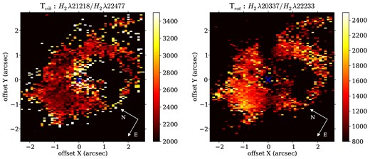
Maps for the vibrational (left-hand panel) and rotational (right-hand panel) temperatures of the H2 emitting gas.
In Fig. 9, we present a plot of |$N_{\rm upp}=\frac{F_i \lambda _i}{A_i g_i}$| (plus an arbitrary constant) versus Eupp = Ti for the locations shown in Fig. 1, namely: (1) the nucleus (left-hand panel), (2) the position corresponding to the peak emission of [Fe ii] (middle panel) and (3) the location of the peak emission of H2 (right-hand panel). The fits of the observed data points by the equation (5) are shown as continuous lines. The fit reproduces the observed data for the three positions and thus confirm that the |$\text{H}_2$| emitting gas is in thermal equilibrium. For the nucleus, the excitation temperature obtained from the fit is ≈2700 K, while for the extra-nuclear regions the excitation temperature is about 2250 K. These values for the excitation temperature of H2 in NGC 1068 are in good agreement with previous estimates of Texc for other Seyfert galaxies (Storchi-Bergmann et al. 2009; Riffel et al. 2010a; Riffel & Storchi-Bergmann 2011b; Schönel Júnior et al. 2013).

Thermal excitation temperature derived from the fluxes of a series of H2 emission lines at the three positions shown in Fig. 1. Ortho transitions are shown as filled circles and para transitions as triangles.
In Storchi-Bergmann et al. (2012), we have performed spectral synthesis of the continuum and concluded that, at the ring, there is a strong contribution of a young but not ionizing, stellar population – the main component being that with age 30 Myr. Particularly conspicuous in the H2 flux distribution and in the young population contribution is the ‘knot’ of strong H2 emission at approximately 1 arcsec E of the nucleus. This region shows a large velocity dispersion, being observed from the channel maps in blueshift centred at −130 km s−1 up to the one in redshift at 112 km s−1 and even at 172 km s−1. One possibility to explain this high velocity dispersion is the presence of supernova remnants there, what would be compatible with the age of the stellar population. In spite of having a larger velocity dispersion than in the rest of the ring, the H2λ2.2477 μm)/λ2.1218 μm line ratio at this location does not differ from those in the remainder of the ring, supporting also thermal excitation there.
Using long-slit spectroscopy of a sample of 67 emission-line galaxies together with photoionization models, Riffel et al. (2013b) have investigated the origin of the H2 line emission and concluded also that heating by X-rays is the dominant thermal process for active galaxies. Our more detailed data suggests that this also happens in NGC 1068: the H2λ2.2477 μm/λ 2.1218 μm ratio also indicates that the H2 emission is mainly due to X-ray heating.
4.4.2 The origin of the [Fe ii] emission
Most of the previous studies referred to in the previous section, address also the excitation mechanisms of the near-IR [Fe ii] emission lines and in general support a larger contribution of excitation by shocks to the [Fe ii] than to the H2 excitation, based mainly on emission-line ratios. However, in Dors et al. (2012), we showed that the [Fe ii] emission in active galaxies can also be reproduced by photoionization models which include only X-rays from the central AGN, even though a contribution from shocks cannot be discarded. On the other hand, Riffel et al. (2013b) found that shocks play an important role in the origin of the [Fe ii] emission in AGNs. Thus, the [Fe ii] origin in AGNs is still an open question to be further investigated.
One interesting property of the [Fe ii] emission in NGC 1068 is the fact that, within the FOV of our observations, its emission is more extended than that of [O iii], as discussed in previous sections. As the Brγ flux distribution seems to be similar to that of [O iii] (see Fig. 3), we have used the channel maps of Brγ (Barbosa et al. 2014) to investigate this difference between the [O iii] and [Fe ii] emitting gas also regarding their kinematics. What can be seen in the channel maps is that there is a strong similarity between the two in the blueshift channels, although only at the highest flux levels, as the emission in the [Fe ii] map is more extended than that of Brγ. But the most striking difference is observed in the redshift channels, in which little emission is seen in Brγ to the N-NE and S-SW, while in [Fe ii] there is strong emission within the whole quadrant between N and E. Adopting the approximate geometry for the outflow proposed by Das et al. (2006), the origin of this emission in redshift would be the back wall of the conical/hourglass outflow to the NE. Actually, the hourglass shape of the outflow seen in the [Fe ii] flux distribution has an important contribution from this redshifted part of the outflow. But why there is emission from this part in [Fe ii] and not in Brγ? As pointed out by Mouri, Kawara & Taniguchi (2000), the [Fe ii] emission is excited by electrons in a zone of partially ionized H. This zone is found around AGN because it is formed when the H ionizing photons have been already absorbed but there is heating of the gas by X-rays and/or shocks, that can still ionize the Fe i. This explains why we see a lot of [Fe ii] emission and little Brγ emission from the back part of the outflow: most of this region is a partially ionized zone.
Further investigation on the origin of the [Fe ii] emission can be done via the line ratios shown in Fig. 5. In particular, the [Fe ii] λ1.2570 μm and [P ii] λ1.1885 μm emission lines have similar excitation temperatures, with their parent ions having similar ionization potential and radiative recombination coefficients. In H ii regions, where shocks are not important, the ratio [Fe ii]/[P ii] is ≈ 2. In supernova remnants, fast shocks destroy the dust grains and release the Fe, increasing its abundance and thus its emission (e.g. Oliva et al. 2001; Storchi-Bergmann et al. 2009; Riffel & Storchi-Bergmann 2011b; Riffel et al. 2013a), leading to line ratios larger than 20 (Oliva et al. 2001). The same can happen in AGNs, where nuclear jets can produce the shocks. In the top-left panel of Fig. 5, the ratio [Fe ii]/[P ii] ≤ 3 within a circular region with radius 1 arcsec centred ≈0.5 arcsec N of the nucleus, while values of up to 10 are observed further out to the NE and to the SW, along the bipolar outflow observed in [O iii] (Das et al. 2006, 2007), suggesting that shocks are present at these locations. These shocks are probably due to the interaction of the outflowing material and/or the radio jet with ambient gas. Similar behaviour of the [Fe ii] emission has also been observed for other active galaxies (Storchi-Bergmann et al. 2009; Riffel et al. 2010a; Riffel & Storchi-Bergmann 2011b; Riffel et al. 2013a): an enhancement of [Fe ii]/[P ii] line ratio in association with a radio jet.
The [Fe ii] (1.2570 μm)/Paβ line ratio can also be used to investigate the origin of the [Fe ii] emission. Values larger than 2 indicate that shocks contribute to the excitation of the [Fe ii] lines (e.g. Rodríguez-Ardila et al. 2004, 2005; Riffel et al. 2006a; Storchi-Bergmann et al. 2009; Riffel & Storchi-Bergmann 2011b; Riffel et al. 2013a). For NGC 1068, most regions present values smaller than 2 as can be seen in Fig. 5 indicating that X-rays are the main excitation mechanism of the [Fe ii] lines. Nevertheless, some higher values are observed to NE along the bi-cone – at the same location where the Fe ii]/[P ii] presents the highest values – consistent with shock excitation at these locations.
In summary, we conclude that the [Fe ii] near-IR lines are originated from the emission of an outflowing gas excited mainly by X-rays from the central AGN, but also with a contribution from shocks associated with the radio jet to NE and SW of the nucleus.
4.5 Masses of ionized and molecular gas
Integrating the Brγ flux over the NLR, we obtain FBrγ ≈ 1.6 × 10⁻¹⁵ ergs−1cm−2 resulting in |$M_{\rm H\,\small {II}}\approx 2.2\times 10^{4}\,{\rm M_{\odot }}$|, for an electron density Ne = 500 cm−3 – the average Ne we have found in our previous studies (Storchi-Bergmann et al. 2009; Schnorr-Müller et al. 2011, 2014a,b).
The integrated flux of the H2 line is |$F_{\rm H_{2}\lambda 2.1218}\approx 2.5\times 10^{-15}\,{\rm erg\,s^{-1} cm^{-2}}$| for NGC 1068, resulting in a mass of only |$M_{\rm H_2}\approx 29\,{\rm M_{\odot }}$|.
Thus, the mass in ionized gas is about 1000 times larger than the mass in hot molecular gas in the inner 200 pc of NGC 1068. The ratio |$M_{\rm H\,\small {II}}/M_{\rm H_2}$| is similar to those we have found in similar studies of other active galaxies, which ranges from 103 to 104 (Storchi-Bergmann et al. 2009; Riffel et al. 2010a, 2013a).
Using the flux quoted above for the H2λ2.1218 μm line, we obtain |$L_{\rm H_{2}\lambda 2.1218}\approx 6.9\times 37\,{\rm erg\, s^{-1}}=1.8\times 10^{4}\,{\rm L_{\odot }}$| and thus Mcold ≈ 2.1 × 10⁷ M⊙. This value is 106 times larger than that obtained for the mass of hot molecular gas, in agreement with the range quoted above (between 105 to 107; e.g. Dale et al. 2005; Mazzalay et al. 2013a; Riffel et al. 2013a).
5 FINAL REMARKS
We have mapped the emitting gas flux distributions, reddening and excitation of the inner ≈200 pc of NGC 1068, at a spatial resolution of ≈10 pc using near-IR adaptive optics IFS obtained at Gemini with the instrument NIFS. The main conclusions of this paper are as follows.
The emitting H2 and ionized gases have completely different flux distributions. The first is observed in a circumnuclear ring in the plane of the galaxy with radius 75 pc and the latter trace the bipolar outflows previously observed in the optical;
The comparison of line-ratio maps with the values predicted by different excitation models shows that most of the H2 line emission is excited by thermal processes, mainly due to heating of the gas by X-rays from the central AGN to an excitation temperature of 2200 K.
The flux distribution in the H emission lines, such as Brγ, follows that observed in the optical [O iii] emission, previously described as having a bipolar cone-shaped structure; the [Fe ii] flux distribution is nevertheless more extended and shows an hourglass structure, broader than a cone and similar to that seen in planetary nebulae such as NGC 6302.
The broader and more extended flux distribution in the [Fe ii] emission lines is attributed to the fact that the it originates in a partially ionized region, that extends beyond the fully ionized region and is excited mainly by X-rays from the central AGN, with some contribution from shocks to NE and SW of the nucleus along the bi-cone axis. Shock excitation is supported by the enhancement in the [Fe ii](1.2570 μm)/[P ii](1.1885 μm) and [Fe ii](1.2570 μm)/Paβ emission-line ratios, and is attributed to the passage of the radio jet through the NLR;
Reddening maps for the NLR were obtained from H and [Fe ii] emission-line ratios, presenting values in the range 0 ≤ E(B − V) ≤ 2, but with an average value of 0.6, observed at most locations; the highest reddening values are observed at ≈0.8 arcsec north of the nucleus;
The mass of ionized gas in the inner ≈200 × 200 pc2 of NGC 1068 is |$M_{\rm H\,\small {II}}\approx 2.2\times 10^{4}\,{\rm M_{\odot }}$|, while the mass of the H2 emitting gas (hot molecular gas) is only |$M_{\rm H_2}\approx 29\,{\rm M_{\odot }}$|. Considering the average factor between the masses of cold and hot molecular gas observed for AGN in general, the total (dominated by the cold) H2 mass is estimated to be M ≈ 2 × 10⁷ M⊙.
Based on observations obtained at the Gemini Observatory, which is operated by the Association of Universities for Research in Astronomy, Inc., under a cooperative agreement with the NSF on behalf of the Gemini partnership: the National Science Foundation (United States), the Science and Technology Facilities Council (United Kingdom), the National Research Council (Canada), CONICYT (Chile), the Australian Research Council (Australia), Ministério da Ciência e Tecnologia (Brazil) and SECYT (Argentina). This work has been partially supported by the Brazilian institutions CNPq and FAPERGS. This research has made use of the NASA/IPAC Extragalactic Database (NED) which is operated by the Jet Propulsion Laboratory, California Institute of Technology, under contract with the National Aeronautics and Space Administration.
