


Abstract
We use MERLIN, VLA and VLBA observations of Galactic H i absorption towards 3C 138 to estimate the structure function of the H i opacity fluctuations at au scales. Using Monte Carlo simulations, we show that there is likely to be a significant bias in the estimated structure function at signal-to-noise ratios characteristic of our observations, if the structure function is constructed in the manner most commonly used in the literature. We develop a new estimator that is free from this bias and use it to estimate the true underlying structure function slope on length-scales ranging from 5 to 40 au. From a power-law fit to the structure function, we derive a slope of |$0.81^{+0.14}_{-0.13}$|, i.e. similar to the value observed at parsec scales. The estimated upper limit for the amplitude of the structure function is also consistent with the measurements carried out at parsec scales. Our measurements are hence consistent with the H i opacity fluctuation in the Galaxy being characterized by a power-law structure function over length-scales that span six orders of magnitude. This result implies that the dissipation scale has to be smaller than a few au if the fluctuations are produced by turbulence. This inferred smaller dissipation scale implies that the dissipation occurs either in (i) regions with densities ≳ 103cm−3 (i.e. similar to that inferred for ‘tiny scale’ atomic clouds or (ii) regions with a mix of ionized and atomic gas (i.e. the observed structure in the atomic gas has a magnetohydrodynamic origin).
1 INTRODUCTION
The neutral atomic hydrogen (H i) component of the Galactic interstellar medium (ISM) is observed to have structure on a wide range of spatial scales. Studies over the last several decades have shown that this structure can be characterized by a scale-free power spectrum on scales varying from a fraction of a parsec to hundreds of parsecs (Crovisier & Dickey 1983; Green 1993; Deshpande, Dwarakanath & Goss 2000; Dickey et al. 2001; Roy et al. 2009). This is generally understood to be the result of compressible fluid turbulence in the ISM. The turbulence is in turn believed to be generated by supernova shock waves, spiral density waves in the disc, etc. (see, e.g. Elmegreen & Scalo 2004; Scalo & Elmegreen 2004, for reviews). In addition to this parsec-scale structure, fine scale structure on scales of tens of au have also been observed in the atomic ISM (Dieter, Welch & Romney 1976; Davis, Diamond & Goss 1996; Faison & Goss 2001; Brogan et al. 2005; Lazio et al. 2009; Stanimirović et al. 2010). However, the connections, if any, between these au-scale structures and the structures observed at larger scales are not well understood. The existence of ubiquitous au-scale structure implies either that these structures are long lived and are in pressure equilibrium with the much lower (typically orders of magnitude smaller) density gas surrounding them, or that they are being continuously created (Hennebelle & Audit 2007). Recent numerical simulations (Nagashima, Inutsuka & Koyama 2006; Vázquez-Semadeni et al. 2006; Hennebelle & Audit 2007) suggest different mechanisms for generating and sustaining these au-scale structures. An alternative model proposed by Deshpande (2000) postulates that the observed fine scale structure is the projection of larger scale structures in the plane of the sky. In this picture, the au-scale structure would form part of the same scale-free structure observed at parsec scales.
Here, we use combined MERLIN,1 VLA2 and VLBA3 observations to estimate the structure function of the H i absorption towards 3C 138. Monte Carlo simulations show that the noise bias in the structure function, estimated from data with low signal to noise, is significant and is also scale dependent. We develop a new estimator that is free from this bias and use this to estimate the true underlying structure function on au scales. Finally, we compare the structure function that we measure on these small scales with that determined at larger scales.
2 STATISTICAL DESCRIPTION OF THE OPTICAL DEPTH FLUCTUATIONS
2.1 Formalism
2.2 Measurement of the optical depth fluctuation
2.3 The effect of measurement noise on the estimated structure function
2.4 Description of the data
Our analysis is based a combined data set obtained from MERLIN, VLA and VLBA observations4 of 3C 138. Details of the different data sets used to make this image, as well as the data analysis procedure followed, are presented by Roy et al. (2012). To summarize, a spectral data cube was made from the combined calibrated uv-data using multi-scale clean. The data cube has a spectral resolution of 0.4 km s−1 per channel and a spatial resolution of 20 mas with rms noise per channel about 20 mJy. The source is unresolved in the VLA observations, so the VLA data allow us to accurately measure the total flux density. Further, the MERLIN, VLA and VLBA have overlapping baselines. The combined data set hence samples all angular scales between the total extent of the source (∼500 mas) and the largest angular scale probed by the VLBA (∼6 mas). Fig. 1 shows the average Galactic H i optical depth spectra towards 3C 138.
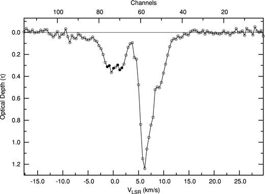
Average Galactic H i optical depth spectrum along the line of sight of 3C 138 from the combined MERLIN, VLA and VLBA data set is plotted against the LSR velocities. The corresponding channel numbers are marked on the top axis. The channels for which the structure function could be measured (see Section 4) are marked by filled circles in the velocity range −1.2 to 1.7 km s−1.
3 MONTE CARLO SIMULATIONS
For running the simulations, we need three main input parameters: the amplitude and slope of the fluctuation power spectrum, and the mean value of the optical depth. Several previous studies (e.g. Deshpande 2000; Roy et al. 2010) have found that the power spectrum of H i opacity fluctuations in the Milky Way, as well as in external galaxies, is well described by a power law with slope ∼−2.6 to ∼−2.8. Based on this, we assume that Pτ(U) = A Uα, with α = −2.7 and A = 1.0 × 10¹⁸ (U in rad−1). This value of the power spectrum amplitude A is chosen so that the amplitude of the simulated structure function is comparable to the observed structure function (see below).
Keeping A and α fixed to the above values, 64 different realizations of |$\tau ^{(\rm S)}({\boldsymbol {\theta }})$| images were generated for different |$\tau ^{(\rm M)}_{0}$| values ranging between 0.1 and 1.0. The mean and the standard deviations of the averaged optical depth values from these realizations are plotted against the known true |$\tau ^{(\rm M)}_{0}$| in Fig. 2. The dashed line is the expected relation from equation (9) and can be seen to agree well with the results from the simulation. In the rest of the paper, we have used this curve to determine the value of input |$\tau ^{(\rm M)}_{0}$| to use with a particular simulation.
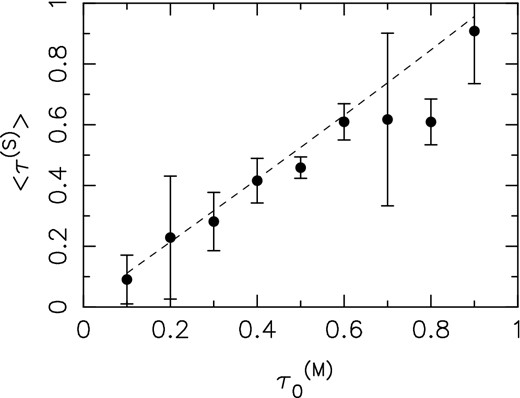
The average optical depth |$\langle \tau ^{(\rm S)}({\boldsymbol {\theta }}) \rangle$| as measured from the simulated optical depth images as a function of the true mean optical depth in the simulation |$\tau ^{(\rm M)}_{0}$|. The optical depth fluctuations are assumed to follow a power law with amplitude A = 1.0 × 10¹⁸ and slope α = −2.7. The averages and standard deviations are determined over 64 different realizations. The dashed line is the expected analytical relation (equation 9).
To illustrate the effect of the bias in the measured structure function, we show in Fig. 3 the results from 128 simulation runs with the optical depth power spectrum amplitude fixed to A = 1.0 × 10¹⁸ and slope α = −2.7 as before and the mean optical depth set to |$\tau ^{(\rm M)}_{0}= 0.4$|. For each simulated image, we estimate the structure function of the optical depth fluctuations. These structure functions are plotted in Fig. 3 as grey lines. The average structure function of the 128 realizations is also shown as a dark continuous line. For comparison, the structure function computed from a single line channel of the actual data cube is shown as a dashed line and the true underlying structure function (which has slope β = −(2 + α) = 0.7) is shown as a dot–dashed line. The steep rise in the measured structure function at angular scales below 0.01 arcsec reflects the fact that the pixel values are highly correlated for separations smaller than the resolution. The large scatter in the different structure functions at large angular scales is due to the fact that there are only a few measurements at large separations. At intermediate scales, the measured structure function is consistent with a power law, but with a shallower slope than the true structure function. This effect illustrates the bias that was discussed in the previous section. As can be seen, the structure function estimated from the observed data is well matched by the structure functions estimated from the simulated data.
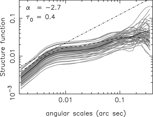
Structure function estimated from 128 realizations with α = −2.7 and τ0 = 0.4 is plotted against the angular scales (grey curves). Mean of these realizations is also plotted (black curve). The dot–dashed line has the same slope as the noise-free structure function. For comparison, the structure function estimated from one of the line channels with average optical depth ∼0.4 from the data is also plotted.
3.1 An unbiased estimator for the slope of the structure function
In this section, we use the simulation procedure described above to construct an unbiased estimator |$\hat{\beta }$| for the structure function slope β. We start by noting from equation (6) that the bias in the observed optical depth is half of its variance. Hence, the bias is reduced if the structure function is estimated from the pixels in the optical depth image with a high SNR. Restricting the measurement to only high SNR pixels, on the other hand, will also reduce the number of usable pixels. This procedure could also result in other more complicated biases by selectively sampling only part of the entire image. To determine the optimum value of SNR as a cutoff, we have applied different SNR cutoffs to the simulated optical depth images, and investigated which cutoff allows us to recover the input structure function.
As before, we set the optical depth fluctuation power spectrum amplitude and slope to A = 1.0 × 10¹⁸ and α = −2.7, respectively, and the mean optical depth to be |$\tau ^{(\rm M)}_{0}= 0.4$|. As discussed in more detail below, we chose |$\tau ^{(\rm M)}_{0}= 0.4$| in order to maximize the number of pixels in the final image with SNR greater than the cutoff. We then compute the structure function from these images, using only pixels above a given threshold SNR value (TSNR). Next, we fit a power law (S0 ϕβ) in the angular scale range of 0.01–0.05 to the structure function estimated from each simulation and estimate the value of β for each run. We exclude the values of β for which the fractional error from the fit is larger than 20 per cent (i.e. SNR less than 5). The mean and standard deviation are then calculated over the remaining realizations of the β values. We repeat this procedure for different values of TSNR. Fig. 4 shows the mean and standard deviation of the recovered β values for different values of TSNR. The dashed line corresponds to the true value of β. Naively, higher TSNR is expected to improve the accuracy in the estimate of β. However, since high optical depth pixels also correspond to low SNR, the number of high optical depth pixels available to estimate β decreases as the TSNR increases. This leads to a flattening of the structure function (or equivalently a decrease in β) as TSNR is increased. As can be seen, at TSNR = 3 the recovered β is close to the true one; for higher and lower values of TSNR the recovered β is offset from the true value. So at least for an input structure function slope of 0.7, a cutoff value of TSNR ∼ 3 is optimal. To check whether it is optimal for other input structure function slopes, the same procedure is repeated for different values of α, viz. −3.0 < α < −2.1 (i.e. 1.0 > β > 0.1). The results are summarized in Fig. 5, where the distribution of |$\widehat{\beta }$| for each input β is shown in the form of a boxplot. The solid horizontal line (cross) inside each boxplot represents the median (mean) of the distribution of |$\widehat{\beta }$|. For β ≳ 0.4, using a cutoff of TSNR = 3 results in a value of |$\widehat{\beta }$| that is close to β. For lower values β, even with a cutoff TSNR = 3, |$\widehat{\beta }$| is systematically offset from β. In the range 0.4 ≲ β ≲ 0.9, the mean value of |$\widehat{\beta }$| is offset from β by a constant, viz. −0.02. So the final step in determining an unbiased value of the structure function slope would be to subtract this constant from |$\hat{\beta }$|. Apart from estimating β, we would also like to know the confidence intervals around the estimated β. We return to this issue after we have applied this estimator to the actual data.
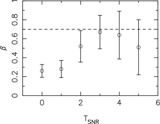
Mean value and the standard deviation (as error bars) of the best-fitting Galactic H i structure function slope estimated from the simulated data are plotted for different signal-to-noise thresholds (TSNR) in the optical depth values. The dashed horizontal line corresponds to an input slope of 0.7. See the text for details.
![Boxplots representing the distributions of $\widehat{\beta }$ for different values of input β. Data boundaries (excluding the outliers) are marked by the bar ends, while the box boundaries mark 25 and 75 per cent quantiles. The mean (crosses) and median (thick solid horizontal lines) from the points excluding the outliers are also shown. The number of data realizations for which $\widehat{\beta }$ could be estimated are [59, 53, 48, 50, 42, 46, 42, 35, 31, 27] (left to right) for the boxplots with input β values from 0.1 to 1.0 respectively.](https://oup.silverchair-cdn.com/oup/backfile/Content_public/Journal/mnras/442/1/10.1093_mnras_stu881/1/m_stu881fig5.jpeg?Expires=1749859504&Signature=MvlFMJQgR~EyulfHnpsd6-TdNKyr566YtVD91iWgOPHERksEBkc8h-drscBQE9QBdfnXdx9VNteDpKJiieOKivjlIx1zOfDRnuGmVk0ax2Wk57oIobCGXUGj0Fo2pIPoyjDiOuNV-u1xWkYVV~kORzlY9V~0Koz8qcWjgy4FGL~oZTfrs0jxntOr4xCZ7qnkX6-4vbx0m-JYqFP5-y1FB-r8cqWCtJwuLiD998xqQVB~akRc4tUk7luDwSvcHX0En42TifiT0QUZdDj5pdUr1TiiQStra3VarLYG-S~0IIb3eoLEMiq8UCif-R2wO-LTbbQ0tZhYwLSabpUID3lGfA__&Key-Pair-Id=APKAIE5G5CRDK6RD3PGA)
Boxplots representing the distributions of |$\widehat{\beta }$| for different values of input β. Data boundaries (excluding the outliers) are marked by the bar ends, while the box boundaries mark 25 and 75 per cent quantiles. The mean (crosses) and median (thick solid horizontal lines) from the points excluding the outliers are also shown. The number of data realizations for which |$\widehat{\beta }$| could be estimated are [59, 53, 48, 50, 42, 46, 42, 35, 31, 27] (left to right) for the boxplots with input β values from 0.1 to 1.0 respectively.
The procedure discussed above leads to an unbiased estimate of the structure function slope. Even after using only the high SNR pixels, the amplitude of the structure function, however, still has a bias, which cannot be easily estimated. This noise bias is positive. So, although we cannot estimate the amplitude of the Sτ(θ), we can set an upper limit to the structure function amplitude.
4 APPLICATION TO THE 3C 138 DATA
Guided by the results discussed in Section 3, we used an SNR cutoff TSNR = 3 to estimate the structure function for all channels in the observed data cube with average optical depth lying between 0.2 and 0.4. This restriction in the mean optical depth occurs for the following reason. Since the noise in the optical depth image increases exponentially with optical depth (see equation 6), the SNR is low for pixels with either large or small optical depths. Consequently, channels with large or small average optical depth have very few pixels that lie above the TSNR = 3 cutoff and generally sample a very restricted region of the image. The net result is that too little data are left to make a good estimate of the structure function.
For spectral channels with mean optical depth between 0.2 and 0.4, the structure function was computed. For a total of six channels the structure function could be fitted using a power law of the form Sτ(ϕ) = S0ϕβ with an uncertainty in the slope of less than 20 per cent (Fig. 6). All of these channels are at velocities corresponding to local H i. The data cube also shows absorption at velocities corresponding to the more distant H i with average optical depth values between 0.2 and 0.4. However, in these channels the number of pixels that remained after using an SNR cutoff of three was too small to estimate the structure function. For the six channels for which the structure function could be estimated, the structure function slope was estimated using the unbiased estimator |$\widehat{\beta }$| introduced in Section 3. As discussed in Section 3, the measured amplitude of the structure function S0 is an upper limit to the amplitude of the true structure function amplitude.
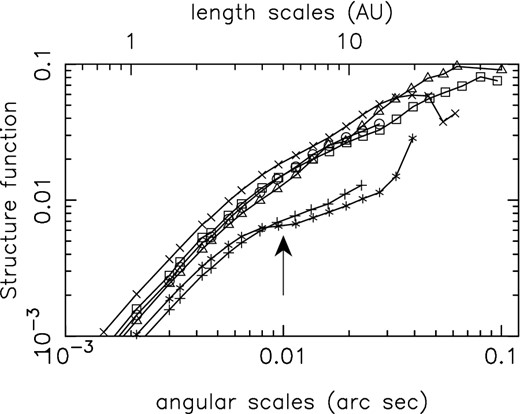
Structure function of Galactic H i estimated using the pixels with 3σ sensitivity in optical depth for the six channels (69, 70, 71, 73, 75, 76). The top axis also shows the corresponding length-scales assuming that the distance to the H i is 500 pc. The instrumental resolution results in a steepening in the structure function at angular scales smaller than 0.01 arcsec. This angular scale is marked by an arrow in the figure.
Fig. 7 shows the resultant values for |$S_{0}, \hat{\beta }$| and the range of angular scales over which the power-law fit was done for the six frequency channels. The top panel of this figure shows the resultant upper limits to the true structure function amplitudes. The middle panel in the same figure shows the slopes of the structure function and the grey bar in the bottom panel gives the range of angular scales for which the estimate could be made. The LSR velocities corresponding to these channels are given in the bottom axis of the plot. The dashed lines in the upper two panels show the amplitude and slope of the optical depth structure function as estimated on parsec scales (Deshpande et al. 2000).

Top panel shows the upper limit of the structure function amplitude estimated from six channels (channel numbers and the corresponding LSR velocities are given at the top and bottom of the figure, respectively) in the data cube. Points with error bars in the middle panel indicate the structure function slope and the grey bars in the bottom panel show the range of angular scales over which the fit could be done. Horizontal lines in the upper two panels indicates the best-fitting value from Deshpande (2000).
All the six channels used to estimate the structure function are shown as filled circles in Fig. 1. For the channels (69, 70, 71), a power law can be fitted over a small range of angular scales (0.01–0.03), whereas for the channels (75, 76), the range is comparatively broader (0.01–0.08). Following Faison & Goss (2001), we adopt a distance of 500 pc for the H i that gives rise to the absorption. At this distance, the angular range of the fit corresponds to a linear range of 5–40 au. The angular range used for the fit does not exceed a factor of 10 for any of the channels. As such, while a power law is consistent with the structure function determine from the data, from the data we cannot prove that the structure function has a power-law form. Other functional forms may also provide a good fit.
In the case of the six channels under discussion (see Fig. 1 for the channels analysed), the recovered slope is similar. The mean value of these six observational estimates of β is |$\widehat{\beta }_{\rm obs}= 0.79$| with a standard deviation of 0.06. The error bars shown in Fig. 7 correspond to the error estimates for the power-law fit. The estimated β is well within the range for which the Monte Carlo simulations show that an unbiased recovery of the slope is possible. As discussed in Section 3, in this range the estimator |$\hat{\beta }$| has a small remaining bias of −0.02. Accounting for this, the final mean estimated slope is 0.81.
Given the estimated value of the structure function slope, we now turn to the question of the appropriate confidence interval for this estimate. Determination of the confidence intervals on the estimated |$\widehat{\beta }$| requires knowledge of the probability distribution of the estimator. To get some information on the probability distribution, we simulated a large number (2048) of images with input β = 0.81 and estimate β using the same procedure as used for the actual data. We denote the estimated standard deviation of this sample by |$\widehat{\mathsf {se}}$|. Given |$\widehat{\mathsf {se}}$|, there are two prescriptions for (1 − γ) confidence intervals (0 ≤ γ ≤ 1) based on the following two different assumptions:
- Assuming that the distribution of |$\widehat{\beta }$| is Gaussian with mean |$\overline{\beta }$| and estimated standard deviation |$\widehat{\mathsf {se}}$|, the (1 − γ) confidence interval on |$\overline{\beta }$| iswhere zx = Φ−1(1 − x) for 0 ≤ x ≤ 1, and |$\Phi (x) = 0.5\, (1 + {\rm erf}(x/\sqrt{2}))$| is the cumulative distribution function for the standard (i.e. zero mean and unit standard deviation) Gaussian distribution. We call this the Gaussian-based confidence interval.\begin{equation*} \overline{\beta } \pm z_{\gamma /2} \times \widehat{\mathsf {se}}, \end{equation*}
Assuming that the distribution of |$\widehat{\beta }$| is unimodal but not necessarily symmetric (or Gaussian), the (1 − γ) confidence interval on β is defined by the γ/2 and (1 − γ/2) numerical quantiles of this sample. We call this the quantile-based confidence interval. In the case when |$\widehat{\beta }$| has a Gaussian distribution, these two prescriptions are equivalent.
Fig. 8 shows the histogram for the estimates of |$\widehat{\beta }$|. The mean value (excluding five potential outliers not shown in the figure) of this distribution (the dashed vertical line) is 0.793, close to the input β. The standard deviation is |$\widehat{\mathsf {se}}=0.138$|. The dashed curve in Fig. 5 shows a Gaussian probability density function with the same mean and standard deviation as the data (excluding the outliers). The confidence intervals using both methods are given in Table 1. As can be seen, both methods provide similar confidence interval of |$0.81^{+0.14}_{-0.13}$| (1σ) on the structure function slope for spatial scales of 5–40 au.
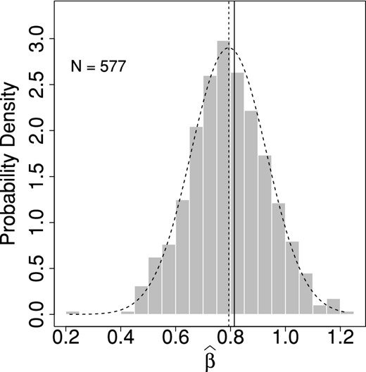
Histogram showing the probability density of |$\widehat{\beta }$| estimated with an input β = 0.81 (input β is indicated with a solid vertical line). The dashed vertical line indicates the mean of the histogram. The mean (dashed vertical line) and median are similar. For comparison, a Gaussian function with same mean and standard deviation of the data is also overplotted (dashed bell-shaped curve). The total number of realizations used to produce the histogram is N = 577.
Quantile- and Gaussian-based confidence intervals for β at the 1σ, 2σ and 3σ levels. Columns (1), (2) and (3) gives the value of γ (see text) and the corresponding quantile- and Gaussian-based confidence intervals.
| γ | Quantile-based | Gaussian-based |
|---|---|---|
| 0.3173 (1σ) | 0.68-0.95 | 0.68-0.95 |
| 0.0455 (2σ) | 0.54-1.08 | 0.54-1.09 |
| 0.0027 (3σ) | 0.48-1.18 | 0.40-1.23 |
| γ | Quantile-based | Gaussian-based |
|---|---|---|
| 0.3173 (1σ) | 0.68-0.95 | 0.68-0.95 |
| 0.0455 (2σ) | 0.54-1.08 | 0.54-1.09 |
| 0.0027 (3σ) | 0.48-1.18 | 0.40-1.23 |
5 DISCUSSION AND CONCLUSION
Deshpande et al. (2000) and Roy et al. (2009) have estimated the H i opacity fluctuation power spectra and/or the structure function in the ISM of our Galaxy. Deshpande et al. (2000) used a very similar image-based technique to estimate the opacity fluctuation structure function towards Cas A. Those authors have not made any correction for the bias, which is justifiable in their case because the brightness of Cas A is expected to make the bias small. This small bias in the case of Cas A is confirmed by the fact that a completely different visibility based approach (which does not suffer from this bias) gives a structure function slope that is in excellent agreement with the image-plane-based approach (Roy et al. 2009). Interestingly, the current measurement of the structure function slope |$\beta = 0.81^{+0.14}_{-0.13}$| (1σ, Gaussian based) at length-scale 5–40 au is consistent with that observed towards Cas A (β = 0.75 ± 0.25) over almost six orders of larger scales (i.e. ∼0.02 to ∼4 pc). The amplitude from the power law given by Deshpande (2000, indicated in the top panel of Fig. 7 by a dashed line) is also consistent with the upper limit derived here.
Roy et al. (2012) also used the same data that are used here to estimate the structure function using a similar technique. The important difference is that Roy et al. (2012) used two methods: (1) no cutoff in optical depth and (2) a 2σ cutoff based on the optical depth signal to noise. This later choice is in contrast to the 3σ signal to noise used in the present analysis. Based on this lower signal-to-noise cutoff, Roy et al. (2012) were able to estimate the structure function over a larger range of angular scale (more than a decade) with 36 spectral channels. On the other hand, as mentioned in Section 4, the 3σ cutoff restricts the analysis to only six spectral channels. The structure function can then be estimated only over a smaller range of angular scales. However, the advantage of the current analysis, demonstrated using the numerical simulations described in Section 3, is that the structure function estimator with the 3σ cutoff is free from the scale-dependent bias arising from the correlated noise. Using a 3σ cutoff is crucial to obtain an unbiased estimator; hence, the present estimate of the structure function slope is more reliable. The current best-fitting value of |$0.81^{+0.14}_{-0.13}$| is consistent with the Roy et al. (2012) value of 0.33 ± 0.07 at roughly a 3σ level. In future, these improved techniques can be applied to data with higher signal to noise in order to estimate the power spectra over a larger range of angular scales and a larger range of velocity channels.
5.1 Turbulence dissipation scale
As mentioned above, our fit of a power-law model for the structure function is over a very small range of angular scales (order of 10). This functional form (viz. a power law) is motivated by the theoretical understanding that fine scale structure is expected to be the result of ISM turbulence and the fact that the structure function on much larger scales is observed to have a power-law form. However, because of the small range of angular scales that we are restricted to in the current analysis, we cannot establish that the structures at these scales actually follow a power law. Nonetheless, we do establish that the data are consistent with au-scale structures having a structure function that has the same slope as that observed on much large scales. In the case of turbulence generated structures in a medium, the structure function assumes a power law at scales lying between the scale of energy input (i.e. the driving scale) and the scale at which energy is taken out (i.e. the dissipation scale). If the structures we see here are generated by turbulence, the turbulence dissipation scale should be smaller than ∼5 au. The dissipation scale for H i in the ISM is discussed in detail by Subramanian (1998). For a largely neutral gas with a thermal velocity dispersion of ∼1 km s−1, and a Kolmogorov-like turbulence, the Reynolds number Re is given by |$R_{e} = 3\times 10^{4}\, \frac{L}{10\, {\rm pc}}\, \frac{v}{10\, {\rm km\, s}^{-1}}\, \frac{n}{1\, {\rm cm^{-3}}}$|. Here, v is the turbulent velocity dispersion, n is the average density at the energy dissipation scale and L is the energy injection scale for turbulence. The dissipation scale ld in such a case is given by |$l_{\rm d} = L R_{e}^{-3/4}$|. Typically, v is ∼5 km s−1 for the neutral gas, and L is ∼10 pc for energy injection via supernova explosions.
Unfortunately, there is no strong or direct constraint on the density at the scales of our interest. If we assume the density to be ∼1–100 cm−3, similar to that of the diffuse cold H i, the dissipation scale is ∼50–1500 au, significantly larger than the 5 au scale probed in the current analysis. In this case, a higher Reynolds number (and hence a smaller dissipation scale) is possible if ionized gas is mixed with the H i (e.g. Brandenburg & Subramanian 2005) and the turbulence is magnetohydrodynamic in nature. On the other hand, if the observed opacity fluctuations are directly related to the so-called tiny-scale atomic structure (TSAS), then the density can be >103 cm−3 (e.g. Heiles 1997), and the dissipation scale for the neutral gas will be ≲ 5 au. The fact that we observe the structure function to be consistent with a power law at au scales hence suggests that either the H i at these scales is associated with ionized gas, and thus the magnetohydrodynamic (MHD) turbulence is playing an important role, or that the observed fluctuations are related to TSAS with a few orders of magnitude higher density.
Complimentary to the radio observations, optical/UV/IR studies have also been used to trace small-scale structures, though these different tracers may not necessarily trace the same ISM phase. Interstellar absorption towards binary or common proper motion systems are used to probe ≲ 2500 au scale. Broadly these observations suggest that while warm gas (traced by, e.g. Ca ii absorption) does not show much structures at these scales, small-scale structures are relatively common in colder gas (traced by, e.g. Na i absorption) at similar scales (e.g. Welty, Hobbs & Kulkarni 1994; Watson & Meyer 1996; Lauroesch & Meyer 2003). Lauroesch, Meyer & Blades (2000) and Lauroesch & Meyer (2003) reported N i structure as small as ∼10–20 au based on observed temporal variation due to proper motion, whereas Rollinde et al. (2003) reported column density structures at similar scales (i.e. ∼10 au) from CH and CH+ observations. Similarly, André et al. (2004) have also reported subpc-scale molecular structure in multiple tracers. Gibson (2007) used optical and radio observations of the Pleiades reflection nebula to reveal a power-law power spectrum of optical dust reflection and H i radio emission with a power-law index of −2.8 over more than five order of magnitude range of scale down to few tens of au. On the other hand, Ingalls et al. (2004) have reported Spitzer observations of the Gum nebula, for which the power spectrum of the surface brightness has a power law with an index of α = −3.5 at milliparsec scales, but α = −2.6 at >0.3 pc scales. Overall however, the optical/UV/IR observations are consistent with the presence of significant self-similar small-scale structures in the ISM.
To summarize, we have used Monte Carlo simulations to show that a direct estimation of the structure function slope from the optical depth image towards 3C 138 is contaminated by a scale-dependent bias. We further show that this bias can be overcome by using only those pixels with SNR greater than three to estimate the structure function. Using this prescription, we have estimated the structure function for absorption from the local gas towards 3C 138, and find that the structure function has a slope of |$0.81^{+0.14}_{-0.13}$| for length-scales from 5 to 40 au. This value of the slope agrees within the error bars with the structure function slope measured on scales that are almost six orders of magnitude larger. The same power-law slope extending down to scales of a few au implies that, if these structures are produced by turbulence, the dissipation scale of the turbulence needs to be smaller than a few au. Finally, we argue that such smaller dissipation scale is consistent with the theoretical models if either the density of these tiny scale structures is more than a few times >103 cm−3, or the H i turbulence is governed by MHD processes via fractional ionization and the presence of magnetic field.
The authors are grateful to K. Subramanian, A. Deshpande, N. Kanekar, S. Bharadwaj and S. Bhatnagar for useful discussions. This paper reports results from observations with MERLIN, VLA and VLBA. MERLIN is a National Facility operated by the University of Manchester at Jodrell Bank Observatory on behalf of PPARC/STFC. The National Radio Astronomy Observatory is a facility of the National Science Foundation operated under cooperative agreement by Associated Universities, Inc. PD would like to acknowledge the DST - INSPIRE fellowship [IFA-13 PH-54 dated 2013 Aug 01] used while doing this research. NR acknowledges support from the Alexander von Humboldt Foundation and the Jansky Fellowship of the National Radio Astronomy Observatory. Part of this research was carried out at the Jet Propulsion Laboratory, California Institute of Technology, under a contract with the National Aeronautics and Space Administration.
MERLIN: Multi-Element Radio-Linked Interferometer Network
VLA: Very Large Array
VLBA: Very Long Baseline Array
MERLIN observation date 1993 October 22 and 23; VLA project code AS0410 and TEST, observation date 1991 September 07 and 13; VLBA project code BD0026, observation date 1995 September 10.
See Wang et al. (2006) for a detailed description of how to generate Gaussian random fluctuations with a given power spectrum.
REFERENCES
APPENDIX A: THE BIAS AND VARIANCE OF THE ESTIMATED OPTICAL DEPTH
- the SNR is large, i.e.\begin{equation*} \frac{ \epsilon \, {\rm e}^{\tau (\nu )}}{I_{\rm C}} \ll 1 \,, \end{equation*}
the noise ϵ has a Gaussian distribution with zero mean,
The measurement noise will also affect the estimated amplitude of the structure function. Intuitively, the amplitude of the structure function measured from a noisy image is expected to be higher than the amplitude of the true structure function. We have used detailed analytical calculations to verify that, under the assumptions listed above, the measured structure function at the angular scales of interest is a scaled version (with scale factor greater than 1) of the noise-free structure function. The Monte Carlo simulations presented in the paper (see Fig. A1) also points to such a multiplicative bias in the structure function amplitude. The actual value of the scale factor, which depends sensitively on the noise level, is difficult to estimate from the observations. In presence of this scaling bias, we can estimate the power-law index of the structure function. However, as the scale factor remains unknown, the amplitude of the measured structure function is only an upper limit to the true structure function.
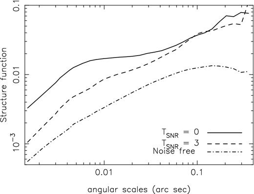
Structure function estimated from one of the 128 realizations of the simulations described in section 3 is plotted for no SNR cutoff (TSNR = 0, solid line) and a cutoff of 3σ (TSNR = 3, dashed line). The underlying noise-free structure function is shown using the dot dashed line. The structure function measured after using a cutoff of 3σ has the same slope as the true structure function. The measured structure function is however biased to higher amplitudes than the true structure function.
