


Abstract
Considering a small misalignment between a point-like source, a singular isothermal ellipsoid deflector and an observer, we derive to first order simple relations between the model parameters and the lensed image positions, and an expression for the time delay between pairs of opposed images which is analogue to the one previously derived for the case of ε − γ models. Combined with the first-order astrometric relations, we retrieve a simple expression for the time delays, in agreement with Witt, Mao & Keeton, which solely depends on the lensed image positions. The real advantage of using the first-order equations when dealing with symmetric gravitational lens systems is to directly test the validity of the adopted lens model without having to perform any accurate numerical fit. In this paper, we present in detail the calculations which lead to those relations between the singular isothermal ellipsoid lens model parameters and the lensed image positions. In addition, we model the well-known Einstein cross Q2237+0305 with three families of models: ε − γ, singular isothermal ellipsoid and non-singular isothermal ellipsoid plus shear, using a genetic algorithm from the Qubist Optimization Toolbox. We conclude that although the non-singular isothermal ellipsoid plus shear model shows the best agreement between the calculated and the observed image positions (〈Δx〉 = 0.0026 arcsec), the more simple singular isothermal ellipsoid also leads to quite satisfactory and acceptable results (〈Δx〉 = 0.0059 arcsec).
1 INTRODUCTION
According to Refsdal (1964a,b), the gravitational lens phenomenon provides a powerful tool to derive the values of several cosmological parameters, i.e. H0, ΩΛ, as well as to deduce the absolute mass of the lensing object, independently on the distance ladder. Unfortunately, such a determination turns out to be model dependent. However, for the case of a small misalignment between the source, the deflector and the observer, Wertz, Pelgrims & Surdej (2012) have recently shown that a first-order perturbative approach applied to the lensed image positions may lead to the determination of the Hubble parameter using observable quantities only (Wertz et al. 2012). Let us note that a similar kind of approach has been developed by Alard (2007) but his singular perturbative method proves to be more restrictive.
The main idea of this paper is to investigate for the case of the singular isothermal ellipsoid (SIE) model whether we can derive first-order equations linking the model parameters to the lensed image positions only. These equations are then used in order to derive model-independent expressions for the time delays between lensed images and the Hubble parameter. Let us note that the derived expressions of H0 are consistent with the ones already presented by Witt, Mao & Keeton (2000).
The outline of this paper is as follows. In Section 2, we recall the basic gravitational lens and astrometric equations for the case of the SIE. We also assume that the lensed images are not resolved individually. Assuming a very small misalignment between the source, the deflector and the observer, we then derive, in Section 3, first-order expressions which link the image positions to the model parameters, as well as the possibility to infer from only observable quantities the value of the Hubble parameter from the linearized astrometric and time delay expressions. Afterwards, we discuss the apparent problem of the degeneracy in determining the value of the parameter ϖ which represents the a priori unknown orientation of the elliptic-shape isodensity contours, and we propose to test the validity range of the astrometric equations. In Section 4, we test the first-order equations for the case of the well-known quadruply imaged quasar: Q2237+0305. We compare the first-order model parameters obtained with those determined numerically using a sophisticated genetic algorithm, called Ferret, which is a component of the Qubist Global Optimization Toolbox (Fiege 2010). Some general conclusions form the last section.
2 THE SINGULAR ISOTHERMAL ELLIPSOID MODEL
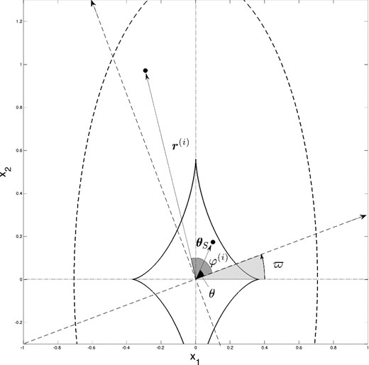
Illustration of the arbitrarily oriented coordinate system which abscissa axis form an angle ϖ with the semiminor axis of the isodensity elliptic contours. The azimuthal angles θ and φ(i) are, respectively, associated with the source and the ith image positions. Both are measured from the arbitrarily oriented coordinate system.
3 FIRST-ORDER EQUATIONS AND SOLUTIONS
3.1 Small deviations from the perfect alignment
3.2 The SIE lens model parameters
In this section, we will recover all lens model parameters from equations (6), (9), (10), (14), (15), (17) and (18). First of all, we need to be careful with the handling of the measured image angular coordinates φ(i). As a reminder, these coordinates are measured from the arbitrarily oriented coordinate system, which implies that φ(i) ∈ [0, 2π]. However, according to the value of ϖ and θ, we may have |$\varphi ^{(i)}_{0} + \Delta \varphi ^{(i)} = {i}\pi /2 - \varpi + \Delta \varphi ^{(i)} < 0$| with i ∈ {0, 1, 2, 3}. Therefore, for (θ + ϖ) ∈ [0, π] and ϖ ∈ [0, Δφ(0)[, we have, to first order, φ(i) = iπ/2 − ϖ + Δφ(i); but for (θ + ϖ) ∈ [0, 2π] and |$\varpi \in [\tilde{\varphi }^{(i)}, \tilde{\varphi }^{(i+1)}]$| with |$\tilde{\varphi }$| representing the image angular coordinate measured from the semiminor axis direction of the isodensity contours, we have φ(k) = kπ/2 − ϖ + Δφ(k) with k ∈ {i + 1, …, 3} and φ(l) ≠ iπ/2 − ϖ + Δφ(l) with l ∈ {0, …, i}. In the latter equation, since the angular quantities are cyclic, the two members are equivalent but not equal. In fact, we have φ(l) = iπ/2 − ϖ + Δφ(l)mod 2π, where mod represents the modulo operation. In the remainder of this section, we will take into account these properties, in particular for the determination of the parameter ϖ.
As a result, we have thus determined the values of f, θS, θ, ϖ and θE from the only astrometric positions of the lensed images. In addition, we note that the index of the lensed images i = {0, 1, 2, 3} is in principle unknown. However, only four possible combinations remain since the index values have to be consecutive. Furthermore, due to the symmetries in the relations between all model parameters and the lensed image positions (see equations 20, 23, 24, 27 and 28), we note that the inversion between the index of two opposed lensed images does not have any impact on their determination: 0↔2 and 1↔3. In order to differentiate the two remaining combinations |$( 02 \stackrel{?}{\leftrightarrow } 13)$|, we only need to calculate the value of f from equation (27). Indeed, one combination leads to f < 1 while the other one to f > 1, which points towards a non-physical situation of having the minor axis larger than the major one.
3.3 The degeneracy affecting the value of ϖ
For each pair of these parameters and the already determined values of f, θS and θE, we derive eight sets of four lensed image positions. By comparison with the real lensed image positions, there only remain two pairs of parameters: the real one (ϖreal, θreal) and another one which leads to the same lensed image positions. Due to the symmetry of the SIE lens models which leads to a diamond-shaped tangential caustic curve, and for fixed values of f, θS and θE, the two pairs of parameters (ϖ, θ) and (ϖ +, θ) rigorously lead to the same lensed image positions. As a consequence, among the eight different remaining combinations of parameter pairs (ϖl, θlk), the only valid ones are (ϖreal, θreal) and (ϖreal +, θreal). We thus find that the parameter θreal is unequivocally determined.
3.4 Time delays and the Hubble parameter
3.5 Validity range of the first-order equations
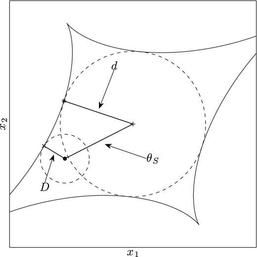
Illustration of the different angular distances involved in the test of the validity range of the first-order equations (see text).
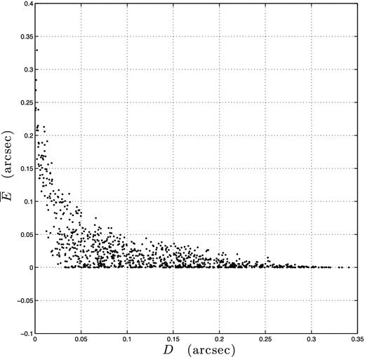
For a set of 1000 model parameters randomly chosen and θE = 1 arcsec, we have represented the distribution of the mean error |$\overline{E}$| between the exact lensed image positions and the derived first order ones as a function of the angular distance between the point-like source and the tangential caustic curve.
In order to further investigate this, we have represented |$\overline{E}$| as a function of the distance D (or θS since these two quantities are correlated) divided by the smallest angular distance d between the tangential caustic curve and the centre of the lens (see Fig. 4). The angular distance d is illustrated in Fig. 2. As shown in Fig. 4, from the same set of the 1000 previous model parameters and for the case θE = 1 arcsec, a more precise condition on the alignment can be derived. For the case of a perfect alignment, i.e. D/d = 1 and θS/d = 0, the mean error |$\overline{E}$| equals zero, as expected. Furthermore, for θS/d < 0.13, the mean error is always such as |$\overline{E} < 0.003$| arcsec which typically corresponds to the error on the observed positions of the lensed images of Q2237+0305. Since the value of d is correlated with the value of f, the latter validity range takes the form θS < 0.13 d(f) where the analytical function d(f) has not yet been determined but could be numerically evaluated.
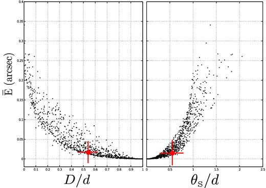
For the same set of 1000 model parameters randomly chosen (see Fig. 3) and θE = 1 arcsec, we have represented the distribution of the mean error |$\overline{E}$| between the exact lensed image positions and the derived first order ones as a function of the normalized distance D/d between the point-like source and the tangential caustic curve (left-hand panel) and as a function of the point-like source radial coordinate θS divided by the smallest distance between the tangential caustic curve and the centre of the lens (right-hand panel). The red crosses correspond to the case of the multiply imaged quasar Q2237+0305.
Furthermore, we have represented, respectively, in Figs 5, 6 and 7 the lensed images, the point-like source, the tangential critical and caustic curves for 12 SIE models and their associated first order ones characterized by θS/d ∈ [0.0, 0.25], θS/d ∈ [0.25, 0.50] and θS/d ∈ [0.50, 1.25], respectively. The model parameters related to those SIE models are given in Tables 1 –3. We notice that as θS/d increases, the accuracy of the first-order SIE model decreases.
![Illustration of different lensed image configurations corresponding to the SIE lens model (open circles ○) and the SIE first order one (pluses +). The source positions associated with the SIE lens model (open square □) and the SIE first order one (cross ×) are also represented. The lens model parameters were randomly chosen such as θS/d(f) ∈ [0, 0.25]. The solid lines correspond to the tangential critical and caustic curves deduced from the SIE lens model, whereas the dashed lines correspond to the SIE first order ones.](https://oup.silverchair-cdn.com/oup/backfile/Content_public/Journal/mnras/442/1/10.1093_mnras_stu866/1/m_stu866fig5.jpeg?Expires=1749872539&Signature=VlsXublo0SO8U8K~rgR53wRIqpTD7mDA44UyHvaswmf9Qf9IWcDrXc-4xJfEceVu3gdvN7KzJopeLm~yd7QR86hGzvpP3kFsIL20TPNvphjAYlfxyHq0oxifpVz4aD84NkRXqWtMQ21Pe3BlGOCaWGfbc1ze3VX2qvX4qZMEYd9sZMyBT150ZedURcJ2LjAqEeRFfgKHVLhf1jCkhF3-gdQIhfveWZoF8f87HqAFyFrAilIC0f6ggkMqP2pda3hi3cZOdlSigLjEXe7dji2m5cBfIx~2lqBlUlN3fnnTW~bE3PjrHfFNsNpYsbzAElqtIur3m6Bs6hRAOUVayh0U7Q__&Key-Pair-Id=APKAIE5G5CRDK6RD3PGA)
Illustration of different lensed image configurations corresponding to the SIE lens model (open circles ○) and the SIE first order one (pluses +). The source positions associated with the SIE lens model (open square □) and the SIE first order one (cross ×) are also represented. The lens model parameters were randomly chosen such as θS/d(f) ∈ [0, 0.25]. The solid lines correspond to the tangential critical and caustic curves deduced from the SIE lens model, whereas the dashed lines correspond to the SIE first order ones.
![Illustration of different lensed image configurations corresponding to the SIE lens model (open circles ○) and the SIE first order one (pluses +). The source positions associated with the SIE lens model (open square □) and the SIE first order one (cross ×) are also represented. The lens model parameters were randomly chosen such as θS/d(f) ∈ [0.25, 0.50]. The solid lines correspond to the tangential critical and caustic curves deduced from the SIE lens model, whereas the dashed lines correspond to the SIE first order ones.](https://oup.silverchair-cdn.com/oup/backfile/Content_public/Journal/mnras/442/1/10.1093_mnras_stu866/1/m_stu866fig6.jpeg?Expires=1749872539&Signature=XQs-uwi4Mk-zhPdwyVO4CPNbTsVo2CQYeyoZL~MTtzrEj7P7jGLNdc1-QXfNqFfZBydzLufW5tgdvt0gCZlw4uxX6YcNpTvKdFzf8OU5fg4AwJ0mhN21hhqVuQMWP~jKh8DS0DAxrHxlgMvQJec9ZddsdjRQBAXLhu-xoWgy-HSmqDQGGpx5awmttaOxrv9jqlcBvsXX~kLUQNCDoFyBp9U4rbSiG0ifvZ20CnDUsRjV91vM2GGQPnt0BQJq-AYYwy~Hvz1VCYK3dPddZRMUWxzJ67aKSV215Jn5ibnyXopJ~9weUMYC7WBi5SPJc8XSv8dP1puBagt6NBuMrAdlVw__&Key-Pair-Id=APKAIE5G5CRDK6RD3PGA)
Illustration of different lensed image configurations corresponding to the SIE lens model (open circles ○) and the SIE first order one (pluses +). The source positions associated with the SIE lens model (open square □) and the SIE first order one (cross ×) are also represented. The lens model parameters were randomly chosen such as θS/d(f) ∈ [0.25, 0.50]. The solid lines correspond to the tangential critical and caustic curves deduced from the SIE lens model, whereas the dashed lines correspond to the SIE first order ones.
![Illustration of different lensed image configurations corresponding to the SIE lens model (open circles ○) and the SIE first order one (pluses +). The source positions associated with the SIE lens model (open square □) and the SIE first order one (cross ×) are also represented. The lens model parameters were randomly chosen such as θS/d(f) ∈ [0.50, 1.25]. The solid lines correspond to the tangential critical and caustic curves deduced from the SIE lens model, whereas the dashed lines correspond to the SIE first order ones.](https://oup.silverchair-cdn.com/oup/backfile/Content_public/Journal/mnras/442/1/10.1093_mnras_stu866/1/m_stu866fig7.jpeg?Expires=1749872539&Signature=bIYLgDGidMkv8mIVmkJmNXvmQ~-Gr9b11E3VduBi2MPKVL4ftm9E~f~WeK5tqiGFAwuGuqf2jqIdarcDhb9EGOFpOysYoqlAXBILhh5PvaYyEZ1hqrJVD8nxTJ5ThbbK3bHXcZD8~xGpOTwe-9Rg6YHNkX~~F1NzjdAQBE89VbjaufbbTvv4N5RHhtsxYbSAS2EfqY18Z8M1AxnKkgBpltM62rkvyMVyv8Emkku41YzCnGeRGEbl35yArJULstvMXk-1VbW7tT783gcap-nOjulxrVbMJnfvvuud-wODICKqo8hO5PQPfPanYYn2WHxKXJRD8OqRdAWz1wfP-7AZgA__&Key-Pair-Id=APKAIE5G5CRDK6RD3PGA)
Illustration of different lensed image configurations corresponding to the SIE lens model (open circles ○) and the SIE first order one (pluses +). The source positions associated with the SIE lens model (open square □) and the SIE first order one (cross ×) are also represented. The lens model parameters were randomly chosen such as θS/d(f) ∈ [0.50, 1.25]. The solid lines correspond to the tangential critical and caustic curves deduced from the SIE lens model, whereas the dashed lines correspond to the SIE first order ones.
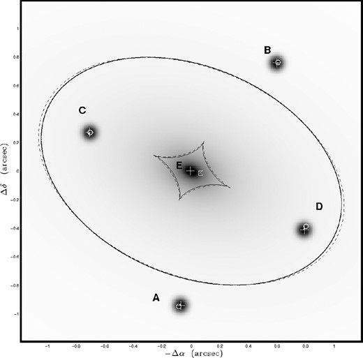
Illustration of the Q2237+0305 gravitational lens system. We have represented the corresponding surface mass density κ(ρ) characterized by the model parameters f and ϖ, as derived from the first-order equations. We have both represented the lensed image positions and the source position, all of them from the model derived by the numerical SIE fitting (see the dots), the NSIE + γ (see the pluses +) and the first-order equations (see the open circles ○). The diamond-shape and ellipse-shape solid lines represent the numerically derived tangential caustic and critical curves, respectively. The diamond-shape and ellipse-shape dashed lines represent the corresponding first-order tangential caustic and critical curves, respectively.
Real and first-order lens parameters for the 12 SIE models represented, respectively, in Fig. 5. For each lens model denoted by #i, we have reported the real model parameters (first line) and the retrieved first order ones (second line).
| Real | f | ϖ | θS | θ | θE | θS/d |
|---|---|---|---|---|---|---|
| first order | ||||||
| #1 | 0.0875 | 0 | 0.0871 | 0.0616 | 0.9807 | 0.1876 |
| 0.0865 | 0.0006 | 0.0871 | 0.0610 | 0.9829 | ||
| #2 | 0.6401 | 0.3307 | 0.0189 | 5.2981 | 0.8911 | 0.1459 |
| 0.6386 | 0.3300 | 0.0189 | 5.2988 | 0.8912 | ||
| #3 | 0.1806 | 0.6614 | 0.0661 | 5.7952 | 1.1218 | 0.1379 |
| 0.1796 | 0.6621 | 0.0661 | 5.7944 | 1.1226 | ||
| #4 | 0.0451 | 0.9921 | 0.0807 | 4.8440 | 1.1944 | 0.1459 |
| 0.0447 | 0.9896 | 0.0806 | 4.8461 | 1.1982 | ||
| #5 | 0.7232 | 1.3228 | 0.0111 | 0.2680 | 0.8120 | 0.1280 |
| 0.7222 | 1.3228 | 0.0111 | 0.2680 | 0.8123 | ||
| #6 | 0.3474 | 1.6535 | 0.0066 | 2.3762 | 1.0143 | 0.0206 |
| 0.3474 | 1.6535 | 0.0066 | 2.3762 | 1.0143 | ||
| #7 | 0.6606 | 1.9842 | 0.0204 | 4.4255 | 0.8348 | 0.1799 |
| 0.6585 | 1.9845 | 0.0204 | 4.4249 | 0.8346 | ||
| #8 | 0.3839 | 2.3149 | 0.0808 | 4.5837 | 1.1208 | 0.2490 |
| 0.3786 | 2.3189 | 0.0805 | 4.5805 | 1.1228 | ||
| #9 | 0.6273 | 2.6456 | 0.0161 | 1.4092 | 1.1957 | 0.0886 |
| 0.6267 | 2.6459 | 0.0161 | 1.4092 | 1.1958 | ||
| #10 | 0.0216 | 2.9762 | 0.0841 | 1.6905 | 0.8268 | 0.2428 |
| 0.0201 | 2.9770 | 0.0841 | 1.6905 | 0.8561 | ||
| #11 | 0.9106 | 3.3069 | 0.0032 | 4.2288 | 1.1758 | 0.0866 |
| 0.9104 | 0.1653 | 0.0032 | 4.2290 | 1.1758 | ||
| #12 | 0.8006 | 3.6376 | 0.0132 | 3.0002 | 0.8073 | 0.2216 |
| 0.7985 | 0.4965 | 0.0132 | 2.9984 | 0.8071 |
Real and first-order lens parameters for the 12 SIE models represented, respectively, in Fig. 6. For each lens model denoted by #i, we have reported the real model parameters (first line) and the retrieved first order ones (second line).
| Real | f | ϖ | θS | θ | θE | θS/d |
|---|---|---|---|---|---|---|
| first order | ||||||
| #1 | 0.0991 | 0 | 0.2414 | 5.5107 | 1.1990 | 0.4278 |
| 0.0900 | 3.1177 | 0.2381 | 5.5227 | 1.2407 | ||
| #2 | 0.4898 | 0.3307 | 0.1029 | 2.2189 | 1.1246 | 0.4061 |
| 0.4760 | 0.3227 | 0.1019 | 2.2266 | 1.1272 | ||
| #3 | 0.1932 | 0.6614 | 0.1655 | 2.8239 | 0.9943 | 0.3977 |
| 0.1835 | 0.6723 | 0.1647 | 2.8129 | 1.0023 | ||
| #4 | 0.8959 | 0.9921 | 0.0176 | 6.0540 | 1.1578 | 0.4151 |
| 0.8916 | 0.9935 | 0.0174 | 6.0528 | 1.1579 | ||
| #5 | 0.0991 | 1.3228 | 0.1054 | 0.2658 | 0.8550 | 0.2619 |
| 0.0946 | 1.3225 | 0.1054 | 0.2658 | 0.8729 | ||
| #6 | 0.0442 | 1.6535 | 0.1491 | 6.1133 | 0.9560 | 0.3372 |
| 0.0397 | 1.6563 | 0.1491 | 6.1134 | 1.0058 | ||
| #7 | 0.5573 | 1.9842 | 0.0798 | 1.1888 | 1.1709 | 0.3628 |
| 0.5475 | 1.9846 | 0.0798 | 1.1881 | 1.1696 | ||
| #8 | 0.7725 | 2.3149 | 0.0309 | 4.1916 | 1.1670 | 0.3102 |
| 0.7679 | 2.3157 | 0.0309 | 4.1888 | 1.1663 | ||
| #9 | 0.3119 | 2.6456 | 0.1569 | 3.6847 | 1.0854 | 0.4288 |
| 0.2983 | 2.6470 | 0.1569 | 3.6828 | 1.0872 | ||
| #10 | 0.1790 | 2.9762 | 0.2080 | 4.2419 | 1.0473 | 0.4640 |
| 0.1630 | 2.9980 | 0.2052 | 4.2355 | 1.0807 | ||
| #11 | 0.3390 | 3.3069 | 0.0958 | 2.2684 | 0.9373 | 0.3204 |
| 0.3301 | 0.1577 | 0.0952 | 2.2732 | 0.9418 | ||
| #12 | 0.2101 | 3.6376 | 0.2070 | 3.8973 | 1.1744 | 0.4328 |
| 0.1940 | 0.5068 | 0.2061 | 3.8979 | 1.2098 |
Real and first-order lens parameters for the 12 SIE models represented, respectively, in Fig. 7. For each lens model denoted by #i, we have reported the real model parameters (first line) and the retrieved first order ones (second line).
| Real | f | ϖ | θS | θ | θE | θS/d |
|---|---|---|---|---|---|---|
| first order | ||||||
| #1 | 0.2578 | 0.3307 | 0.3797 | 5.0953 | 1.0881 | 0.9326 |
| 0.1858 | 0.2560 | 0.3560 | 5.1187 | 1.1923 | ||
| #2 | 0.3317 | 0.6614 | 0.1831 | 3.0445 | 1.0887 | 0.5194 |
| 0.3090 | 0.6805 | 0.1803 | 3.0279 | 1.0997 | ||
| #3 | 0.1522 | 0.9921 | 0.4275 | 4.7548 | 1.1511 | 0.8349 |
| 0.1102 | 0.9129 | 0.4068 | 4.8169 | 1.2520 | ||
| #4 | 0.3480 | 1.3228 | 0.3183 | 2.6204 | 1.0330 | 0.9847 |
| 0.2588 | 1.3930 | 0.2941 | 2.5930 | 1.1025 | ||
| #5 | 0.1217 | 1.6535 | 0.3406 | 6.1059 | 0.8283 | 0.8909 |
| 0.0780 | 1.6678 | 0.3401 | 6.1076 | 1.0078 | ||
| #6 | 0.8842 | 1.9842 | 0.0373 | 6.2076 | 1.1691 | 0.7792 |
| 0.8672 | 1.9807 | 0.0367 | 6.1899 | 1.1725 | ||
| #7 | 0.9300 | 2.6456 | 0.0248 | 2.4434 | 0.9144 | 1.1221 |
| 0.9066 | 2.6410 | 0.0236 | 2.3989 | 0.9173 | ||
| #8 | 0.3424 | 3.6376 | 0.3250 | 4.9287 | 1.0863 | 0.9449 |
| 0.2614 | 0.4324 | 0.3040 | 4.9469 | 1.1578 | ||
| #9 | 0.7360 | 3.9683 | 0.1326 | 5.5470 | 1.1356 | 1.1544 |
| 0.6634 | 0.8327 | 0.1321 | 5.5258 | 1.1241 | ||
| #10 | 0.5449 | 4.6297 | 0.1924 | 3.5078 | 0.9882 | 1.0013 |
| 0.4648 | 1.4665 | 0.1888 | 3.4897 | 1.0290 | ||
| #11 | 0.6862 | 4.9604 | 0.0829 | 3.7628 | 1.0243 | 0.6551 |
| 0.6577 | 1.8069 | 0.0805 | 3.7732 | 1.0266 | ||
| #12 | 0.8936 | 5.2911 | 0.0337 | 0.9354 | 0.9076 | 0.9904 |
| 0.8692 | 2.1485 | 0.0337 | 0.9435 | 0.9040 |
Finally, we have determined exact and first-order time delays, between pairs of lensed images for the first eight simulated models represented in Figs 5–7. For this purpose, we have assumed a spatially flat Λ cold dark matter cosmology with a value H0 = 67.3 ± 1.2 km s−1 Mpc−1 for the Hubble parameter and the matter density parameter Ωm = 0.315 ± 0.017 (Planck Collaboration 2013). We have fixed the redshifts of the simulated sources and lenses according to realistic cases of expected multiply imaged quasars as in Finet (2013). From the normalized redshift distribution of the sources that are detected as multiply imaged, we have selected the most likely redshift of the sources for Ωm = 0.315, i.e. zs = 2.350. For this source redshift, we have calculated the differential contribution to the lensing optical depth as a function of the deflector redshift. We have then selected the most likely deflector redshift corresponding to the maximum of this distribution, i.e. zs = 0.66, as well as those corresponding to the two halves of its maximum, i.e. zs = 0.263 and zs = 1.294. Added to this, we have also considered the source and lens redshifts of the gravitational lens system Q2237+0305. The values of the corresponding time delays are summarized in Tables 4 –6. As expected, we note that the first-order time delays for a pair of opposed lensed images are identical to the exact time delays.
Comparison between the values of the time delays derived from the first-order equations and the real SIE lens model ones. The corresponding lensed image configurations are represented in Fig. 5. The time delays are expressed in days.
| Model | Time delays | Time delays | |||
|---|---|---|---|---|---|
| index | zs | zl | (real) | (to first order) | |
| #1 | 1.695 | 0.039 | Δt01 | 1.95 | 1.97 |
| Δt02 | 0.76 | 0.76 | |||
| Δt03 | 1.97 | 1.99 | |||
| #2 | 1.695 | 0.217 | Δt01 | 3.44 | 3.47 |
| Δt02 | 0.70 | 0.70 | |||
| Δt03 | 2.98 | 3.01 | |||
| #3 | 1.695 | 0.54 | Δt01 | 29.47 | 29.68 |
| Δt02 | 8.59 | 8.59 | |||
| Δt03 | 30.34 | 30.55 | |||
| #4 | 1.695 | 0.97 | Δt01 | 47.91 | 48.32 |
| Δt02 | 14.14 | 14.14 | |||
| Δt03 | 45.19 | 45.60 | |||
| #5 | 2.350 | 0.039 | Δt01 | 0.29 | 0.30 |
| Δt02 | −0.002 | −0.002 | |||
| Δt03 | 0.37 | 0.38 | |||
| #6 | 2.350 | 0.263 | Δt01 | 8.37 | 8.37 |
| Δt02 | −0.25 | −0.25 | |||
| Δt03 | 8.15 | 8.15 | |||
| #7 | 2.350 | 0.66 | Δt01 | 6.32 | 6.40 |
| Δt02 | 2.04 | 2.04 | |||
| Δt03 | 6.55 | 6.63 | |||
| #8 | 2.350 | 1.294 | Δt01 | 35.11 | 36.03 |
| Δt02 | 14.47 | 14.47 | |||
| Δt03 | 42.55 | 43.47 |
Comparison between the values of the time delays derived from the first-order equations and the real SIE lens model ones. The corresponding lensed image configurations are represented in Fig. 6. The time delays are expressed in days.
| Model | Time delays | Time delays | |||
|---|---|---|---|---|---|
| index | zs | zl | (real) | (to first order) | |
| #1 | 1.695 | 0.039 | Δt01 | 1.11 | 1.33 |
| Δt02 | −1.89 | −1.89 | |||
| Δt03 | 2.00 | 2.23 | |||
| #2 | 1.695 | 0.217 | Δt01 | 3.27 | 3.79 |
| Δt02 | −5.12 | −5.12 | |||
| Δt03 | 5.96 | 6.48 | |||
| #3 | 1.695 | 0.54 | Δt01 | 13.63 | 15.00 |
| Δt02 | −18.32 | −18.32 | |||
| Δt03 | 9.81 | 11.18 | |||
| #4 | 1.695 | 0.97 | Δt01 | 5.28 | 5.68 |
| Δt02 | 2.99 | 2.99 | |||
| Δt03 | 8.03 | 8.43 | |||
| #5 | 2.350 | 0.039 | Δt01 | 1.00 | 1.06 |
| Δt02 | −0.01 | −0.01 | |||
| Δt03 | 1.40 | 1.46 | |||
| #6 | 2.350 | 0.263 | Δt01 | 6.02 | 6.54 |
| Δt02 | 0.55 | 0.55 | |||
| Δt03 | 8.57 | 9.09 | |||
| #7 | 2.350 | 0.66 | Δt01 | 9.40 | 10.26 |
| Δt02 | −11.46 | −11.46 | |||
| Δt03 | 9.11 | 9.97 | |||
| #8 | 2.350 | 1.294 | Δt01 | 13.39 | 13.87 |
| Δt02 | 6.62 | 6.62 | |||
| Δt03 | 14.75 | 15.23 |
Comparison between the values of time delays derived from the first-order equations and the real SIE lens model ones. The corresponding lensed image configurations are represented in Fig. 7. The time delays are expressed in days.
| Model | Time delays | Time delays | |||
|---|---|---|---|---|---|
| index | zs | zl | (real) | (to first order) | |
| #1 | 1.695 | 0.039 | Δt01 | 4.66 | 5.32 |
| Δt02 | 2.62 | 2.62 | |||
| Δt03 | 2.69 | 3.35 | |||
| #2 | 1.695 | 0.217 | Δt01 | 6.99 | 8.04 |
| Δt02 | −8.98 | −8.98 | |||
| Δt03 | 3.09 | 4.14 | |||
| #3 | 1.695 | 0.54 | Δt01 | 64.40 | 71.77 |
| Δt02 | 47.63 | 47.63 | |||
| Δt03 | 49.56 | 56.93 | |||
| #4 | 1.695 | 0.97 | Δt01 | 33.93 | 44.81 |
| Δt02 | −46.41 | −46.41 | |||
| Δt03 | 0.21 | 11.09 | |||
| #5 | 2.350 | 0.039 | Δt01 | 0.74 | 1.26 |
| Δt02 | 0.23 | 0.23 | |||
| Δt03 | 2.11 | 2.63 | |||
| #6 | 2.350 | 0.263 | Δt01 | 0.31 | 0.71 |
| Δt02 | −0.77 | −0.77 | |||
| Δt03 | 2.54 | 2.94 | |||
| #7 | 2.350 | 0.66 | Δt01 | 3.13 | 3.62 |
| Δt02 | 0.81 | 0.81 | |||
| Δt03 | 0.82 | 1.31 | |||
| #8 | 2.350 | 1.294 | Δt01 | 77.74 | 88.43 |
| Δt02 | 42.18 | 42.18 | |||
| Δt03 | 43.04 | 53.73 |
4 APPLICATION TO A REAL CASE: Q2237+0305
The gravitational lens Q2237+0305 consists of a quadruply imaged QSO at z = 1.695, discovered by Huchra et al. (1985) in the CfA Redshift Survey of Galaxies. The deflector which leads to the formation of the lensed images is a nearby 15 mag face-on spiral galaxy, at z = 0.0394 (e.g. Schmidt, Webster & Lewis Geraint 1998). Due to its proximity, the lensing galaxy has already been explored in detail. Different approaches have been applied to model this system, e.g. a constant mass-to-light ratio (Schneider et al. 1988; Rix, Schneider & Bahcall 1992; Chae, Khersonsky & Turnshek 1998; Keeton & Kochanek 1998) or multiparametric models (e.g. a de Vaucouleurs law and King profile, Kent & Falco 1988; singular isothermal sphere and point mass along with external shear, Kochanek 1991; a singular power-law axially symmetric deflector with an external shear, Wambsganss & Paczyński 1994; a non-singular power-law density for the distribution of mass, Chae et al. 1998). The astrometric positions of the four lensed images of Q2237+0305, which come from the CASTLES1 survey, are listed in Table 7.
The lensed image positions for the Q2237+0305 system from the CASTLESa survey.
| −Δα | Δδ | |
|---|---|---|
| (arcsec) | (arcsec) | |
| A | 0.0 | 0.0 |
| B | 0.673 ± 0.003 | 1.697 ± 0.003 |
| C | −0.635 ± 0.003 | 1.210 ± 0.003 |
| D | 0.866 ± 0.003 | 0.528 ± 0.003 |
| G | 0.075 ± 0.004 | 0.939 ± 0.003 |
| −Δα | Δδ | |
|---|---|---|
| (arcsec) | (arcsec) | |
| A | 0.0 | 0.0 |
| B | 0.673 ± 0.003 | 1.697 ± 0.003 |
| C | −0.635 ± 0.003 | 1.210 ± 0.003 |
| D | 0.866 ± 0.003 | 0.528 ± 0.003 |
| G | 0.075 ± 0.004 | 0.939 ± 0.003 |
Optimal SIE and ε − γ lens parameters for the Q2237+0305 system, derived by the ferret sophisticated genetic algorithm which is a component of the Qubist Global Optimization Toolbox.
| SIE | SIE | ε − γ | ε − γ | NSIE + γ | |
|---|---|---|---|---|---|
| first order | first order | ||||
| |$\chi ^{2}_{r}$| | 1.5466 | 12.204 | 18.165 | – | 0.7319 |
| f | |$0.6649_{-0.0094}^{+0.0100}$| | |$0.6479_{-0.0097}^{+0.0097}$| | – | – | |$0.6634_{-0.0096}^{+0.0110}$| |
| ϖ | |$1.9720_{-0.0029}^{+0.0028}$| | |$1.9686_{-0.0024}^{+0.0024}$| | – | – | |$2.0111_{-0.0023}^{+0.0023}$| |
| ε | – | – | |$0.6653_{-0.0094}^{+0.0100}$| | 1.5949 | – |
| γ | – | – | |$0.1047_{-0.0094}^{+0.0100}$| | -0.0292 | |$0.0138_{-0.00012}^{+0.00012}$| |
| ω | – | – | |$2.7437_{-0.0094}^{+0.0100}$| | 1.1729 | |$2.7107_{-0.0010}^{+0.0010}$| |
| θS | |$0.0652_{-0.0021}^{+0.0021}$| | |$0.0669_{-0.0035}^{+0.0035}$| | |$0.0595_{-0.0094}^{+0.0100}$| | -0.0166 | |$0.0632_{-0.0011}^{+0.0012}$| |
| θ | |$6.1261_{-0.0146}^{+0.0150}$| | |$6.0629_{-0.0408}^{+0.0408}$| | |$6.0589_{-0.0094}^{+0.0100}$| | 6.0524 | |$6.1236_{-0.0118}^{+0.0119}$| |
| θE | |$0.8974_{-0.0023}^{+0.0023}$| | |$0.9024_{-0.0021}^{+0.0021}$| | |$0.8812_{-0.0094}^{+0.0100}$| | 0.8865 | |$0.9396_{-0.0019}^{+0.0019}$| |
| ρc | – | – | – | – | |$0.0332_{-0.0013}^{+0.0013}$| |
| ΔxA | 0.0031 | 0.0163 | 0.0064 | – | 0.0028 |
| ΔxB | 0.0087 | 0.0097 | 0.0082 | – | 0.0020 |
| ΔxC | 0.0082 | 0.0006 | 0.0210 | – | 0.0030 |
| ΔxD | 0.0036 | 0.0268 | 0.0335 | – | 0.0027 |
Notes. The parameters ε represents the slope of the power-law mass distribution, γ the magnitude of the external shear, ω the orientation of the external shear and ρc the size of the core radius in arcsec. The lower and upper limits correspond to the range of the lens parameters used by the genetic algorithm routine. The distances between the lensed images and the modelled images are represented by Δx.
The SIE lens model shows the best agreement with the observed image positions in comparison with the ε − γ model: <ΔxSIE > = 0.0059 arcsec whereas <Δxε−γ > ≃0.0173 arcsec. Therefore, this is what convinces us to use the SIE first-order equations instead of the ε − γ ones. Furthermore, for the case of the ε − γ model, the first-order values of γ and θS appear to be non-physical. However, we note that the determined value of θE is similar for both lens models which seems to indicate that the determination of the Einstein angular radius very slightly depends on the choice of the deflector's family of models. We notice that both sets of lens parameters (SIE and first-order SIE) are quite similar, which leads to the conclusion that the use of the first-order astrometric equations is justified here. For both SIE and first-order SIE models, we have derived the value of θS/d and D/d from the parameters found in Table 8. For the case of SIE, one finds θS/d = 0.5438, D/d = 0.5649, and for the case of first-order SIE, θS/d = 0.5231 and D/d = 0.6054.
The NSIE + γ model shows the best agreement with the observed lensed image positions in comparison with the SIE model: < ΔxNSIE + γ > ≃0.0026 arcsec, which is smaller than the precision of the observed image positions (see Table 7). The large number of independent parameters (NNSIE + γ = 6) and the very high precision on the modelled image positions explain why we have found |$\chi ^{2}_{r} < 1$|. We note that the parameters f, ϖ, θS and θ between the SIE and NSIE + γ models are very similar, which seems to indicate that the NSIE + γ derived numerical solution is the best for this model, i.e. not a local minimum. The addition of a core leads to the appearance of a fifth lensed image, denoted by E, located very close to the gravity centre of the deflector: −Δα = −0.0069 arcsec and Δδ = 0.0018 arcsec. The observational existence of a fifth lensed image has first been reported by Racine (1991), but it has never been independently confirmed. For the case of the SIE, the first-order SIE and the NSIE + γ models, we have illustrated the corresponding lensed image positions in Fig. 8. Furthermore, we have derived the values of the time delays (in hours) and amplification ratio between the lensed image A and the other ones. We have summarized all the information in Table 9. As expected, the comparison between the values of the time delay ΔtAB (resp. ΔtCD) for the case of the SIE and the first-order SIE models are extremely close. Indeed, we have shown that the first-order time delay expression (equation 38) is identical to the one derived by Witt et al. (2000). Since equation (38) remains valid without any approximation for any pairs of lensed images, equation (35) seems to be useless. However, the SIE (resp. ε − γ) first-order equations (20), (23), (24), (27) and (28) have the advantage to test straightforwardly, and without any numerical simulations, to what extent the SIE (resp. ε − γ) family of models constitutes a good choice and therefore whether the derived values for the time delays and amplification ratios are trustworthy. Without using these first-order equations, equation (38) could still be applied to any symmetric quadruply imaged quasar but without the immediate confidence that the SIE family of models constitutes a good approximation to represent the mass distribution. For Q2237+0305, we have shown that the ε − γ family of models did not properly fit the lensed image positions while the SIE family of models does.
Comparison between the values of the time delays (in hours) and amplification ratios between pairs of lensed images derived from the first-order equations and the real SIE and NSIE + γ models for Q2237+0305.
| SIE | SIE | NSIE + γ | |
|---|---|---|---|
| first order | |||
| ΔtAD/h | −5.3821 ± 0.6841 | −7.2966 ± 0.5278 | −5.4112 ± 0.4291 |
| ΔtAB/h | 2.5992 ± 0.7172 | 2.5983 ± 0.6152 | 2.5080 ± 0.5192 |
| ΔtAC/h | −17.969 ± 0.6969 | −19.877 ± 0.7448 | −18.009 ± 0.6192 |
| ΔtCD/h | 12.587 ± 0.6849 | 12.580 ± 0.6541 | 12.597 ± 0.5812 |
| μB/μA | 0.797 172 | – | 0.84483 |
| μC/μA | −0.184 621 | – | −0.294 92 |
| μD/μA | −0.305 474 | – | −0.490 83 |
| μE/μA | – | – | 0.001 2186 |
Notes. We have fixed the value of the Hubble parameter to 67.3 ± 1.2 km s−1Mpc−1 and the matter density parameter Ωm = 0.315 ± 0.017 (Planck Collaboration 2013).
The values of the estimated time delay listed in Table 9 can be compared with those in Table 10 which constitutes a summary of the model predictions for Q2237+0305. A description of the corresponding lens models may be found in Vakulik et al. (2006). We note that the determination of the time delays depends on the considered models. Unfortunately, the possibility of measuring very accurate time delays between two lensed images from their light curves seems to be very difficult. Different attempts have already been performed (see e.g. Koptelova, Oknyanskij & Shimanovskaya 2006; Vakulik et al. 2006) but none of them allows the authors to definitely conclude. The uncertainties obtained, which correspond to a 95 per cent confidence level, exceed 100 per cent. Therefore, we are not able to compare the measured and the predicted time delays. In order to estimate the value of the Hubble parameter with, at least, the same precision as the Planck Collaboration (2013), we have calculated that the uncertainties on ΔtAB and ΔtCD should be, respectively, smaller than σAB ≤ 0.0465 h (i.e. 2.8 min) and σCD ≤ 0.225 h (i.e. 13.5 min).
Model predictions for the time delays (in hours) ΔtAB, ΔtAC and ΔtAD for Q2237+0305.
| Reference | Lens model | ΔtAB/h | ΔtAC/h | ΔtAD/h |
|---|---|---|---|---|
| Schneider et al. | Constant | 2.4 | 29.5 | 26.6 |
| (1988) | mass-to-light ratio | |||
| Best fit | 0.54 | −6.48 | −6.12 | |
| Model 1 | −2.1 | −11 | −7.1 | |
| Rix et al. (1992) | Model 2 | −1.5 | −10.1 | −6.1 |
| Model 2a | 1.7 | −9.8 | −3.7 | |
| Best fit | 1.3 | −7.4 | −2.8 | |
| Wambsganss | Point lens | 2.97 | −17.41 | −4.87 |
| & Paczyński | SIS | 1.51 | −8.91 | −2.46 |
| (1994) | Best fit | 0.44 | −2.54 | −0.7 |
| Schmidt et al. | Bar accounted | 2.0 | −16.2 | −4.9 |
| (1998) | ||||
| Chae et al. | Triaxial model | [0.13,3.4] | [−16.6,−0.77] | [−5.5,−0.22] |
| (1998) |
5 CONCLUSIONS
Use of the first-order equations leads to a straightforward method of determining whether the deflector's mass distribution can be modelled with the SIE or ε − γ family of models, without the need of any precise model fitting. We have retrieved the same expression for the time delays between pairs of opposite lensed images as already published by Witt et al. (2000). However, combined with the first-order equations, we could easily estimate the validity of these time delay estimates and the relevance of the use of such a family of models. In order to obtain a mean astrometric error ≤0.003 arcsec, the validity range of the first-order equations has been estimated to be θS < 0.13 d(f) which is similar to the one already deduced for the ε − γ family of models (see Wertz et al. 2012).
Application to the quadruply imaged quasar Q2237+0305 constitutes a very interesting way of comparing the results of accurate SIE modelling with those derived from the first-order equations. We have noticed that the model parameters deduced from the first-order equations and the numerical fit are very closed. This leads to the conclusion that the numerical fit, besides being time consuming, does not bring any significant improvement in this case. The degree of misalignment has been evaluated to θS/d = 0.5438 > 0.13. This latter value allows us to understand why the mean astrometric error <Δx1er order > = 0.0134 arcsec is larger than the 0.003 arcsec which corresponds to the error on the observed positions.
Unfortunately, the uncertainties obtained for the observed time delays between the light curves of pairs of lensed images make any comparison very risky. However, we have shown that in order to derive the Hubble parameter with a high precision requires very accurate values for the time delays. Therefore, we suggest that monitoring the gravitational lens system Q2237+0305 with a very high time sampling should constitute a promising way of determining accurate values of the time delays and a precise determination of the Hubble parameter based upon gravitational lensing.
We thank J. Fiege for gratefully providing his very performing Qubist Global Optimization Toolbox. OW thanks the Belgian National Fund for Scientific Research (FNRS). JS and OW acknowledge support from the Communauté française de Belgique - Actions de recherche concertées - Académie universitaire Wallonie-Europe, from the ESA PRODEX Programme ‘GAIA’, and from the Belgian Federal Science Policy Office.
REFERENCES
Author notes
E-mail: [email protected]
Also Directeur de Recherche honoraire du F.R.S. -FNRS.
