


Abstract
We analyse gamma-ray bursts (GRBs) detected by Fermi/Gamma-Ray Burst Monitor and having single pulse. We fit the light curves with a model having exponential rise and decay parts. We perform a detailed time-resolved spectroscopy using four models: Band, blackbody with a power law (BBPL), multicolour blackbody with a power law (mBBPL) and two blackbodies with a power law (2BBPL). We find that models other than the BBPL give better |$\chi _{\rm red}^2$| for the ‘hard-to-soft’ (HTS) pulses, while for the ‘intensity tracking’ (IT) pulses, the BBPL model is statistically as good as the other models. Interestingly, the energy at the peak of the spectrum resulting from the BBPL model (∼3kT) is always lower than that of the νFν spectrum of the Band function. The values of the low-energy photon index (α) of the Band function are often higher than the fundamental single particle synchrotron limit, especially for the HTS pulses. Specifically we find two extreme cases – for GRB 110817A (HTS GRB) α is always higher, while for GRB 100528A (IT GRB) α is always within the synchrotron regime. The power-law component of the BBPL model always starts with a delay compared to the blackbody component, and it lingers at the later part of the prompt emission phase. For three HTS GRBs, namely, GRB 081224, GRB 100707A and GRB 110721A this behaviour is particularly significant and interestingly there are reported Large Area Telescope detections for them. Finally, we argue that various evidences hint that neither BBPL nor Band model is acceptable, while 2BBPL and mBBPL are the most acceptable models for the set of GRBs we have analysed.
1 INTRODUCTION
A gamma-ray burst (GRB) is the most luminous event in the Universe. In a few seconds it produces an enormous amount of electromagnetic energy, which is comparable to the integrated emission of the Sun over 10 billion years (Mészáros 2006). Most of this energy is released in the first few seconds in the form of gamma-rays (keV to MeV), known as the prompt emission phase. In some GRBs very high energy (GeV) emission is also observed during the prompt phase. Later the afterglow of a GRB can be observed at all electromagnetic frequencies from the radio wavelengths up to X-rays and even gamma-rays. Numerous satellite experiments have been performed to pin down the mechanism of GRBs. For 10 long years (1991–2000), a great wealth of prompt emission data was collected by the Burst and Transient Source Experiment (BATSE; Fishman et al. 1994) onboard the Compton Gamma-ray Observatory (CGRO). With Swift (Gehrels et al. 2004; Barthelmy et al. 2005) and Fermi (Meegan et al. 2009), launched, respectively, in 2004 and 2008, we have entered into the modern era of GRB research. Swift, with its fantastic slewing capability, an unprecedented localization accuracy of the primary GRB detector (Burst Alert Telescope – BAT, a large field of view gamma-ray monitor) and the high spatial resolution instruments for the afterglow studies has enabled the measurement of the redshift for many GRBs. Fermi, on the other hand, has enabled a detailed spectral study during the prompt emission phase, and discovered the very high energy (GeV) emission both during the prompt and afterglow phase for many bursts (very few such events were known before Fermi; see e.g. González et al. 2003). Both these satellites have supplied extremely valuable data for the identification of the working mechanism of GRBs. However, even after nearly 50 yr of discovery, various issues remain puzzling, most notably the prompt emission mechanism.
In the preliminary model of a GRB, known as the ‘standard fireball model’ (Goodman 1986; Paczynski 1986), the radiation is supposed to come from a photosphere. The instantaneous spectrum is predicted to be a blackbody (BB) and the light curve (LC) is a simple pulse. Though we do see a GRB having a single pulse, there is a variety of LC profiles. There are also differences in the predicted and observed spectrum. While the BB spectral shape in the photon space is a hump with a narrow peak, which can be approximated with a low-energy power law (PL) with a +1 index and a steep PL with a negative index at high energy, GRB prompt emission spectra usually have non-thermal spectral shape characterized with negative PL indices (∼−1). Though there is a provision for geometric broadening (Goodman 1986), the spectrum is still far from what is observed. To overcome this difficulty, it is assumed that the radiation is not coming from the photosphere, but it is produced in the internal shocks (ISs) of the ejecta via synchrotron radiation (Rees & Mészáros 1994; Woods & Loeb 1995; Kobayashi, Piran & Sari 1997; Sari & Piran 1997). This model is phenomenologically represented by the featureless Band function (Band et al. 1993), which is a smoothly joined PLs with two indices – α as the lower energy index and β as the higher energy index. In the EF(E) representation, the function peaks at an energy (Epeak), provided that β < −2, which can be violated for very hard spectra. The prompt emission data, whether time integrated or time resolved, are adequately fit by the Band function (Kaneko et al. 2006; Nava et al. 2011; Zhang et al. 2011). However, the Band function is a phenomenological function and the actual spectrum may have rich structure. In many studies, additional components to the Band function (Preece et al. 1996; Mészáros & Rees 2000; González et al. 2003; Shirasaki et al. 2008; Abdo et al. 2009, Ackermann et al. 2010, 2011; Guiriec et al. 2011, 2013; Axelsson et al. 2012) and even alternative models (Ghirlanda, Celotti & Ghisellini 2003; Ryde 2004; Ryde & Pe'er 2009; Pe'er & Ryde 2011) have been suggested. The reason for resorting to alternative description is that the IS model demands that in the electron slow cooling regime, the photon index (α) should be less than −2/3 (Preece et al. 1998), the single particle synchrotron limit. GRBs are usually expected to be in the fast cooling regime where the photon index should be near −3/2 (Cohen et al. 1997). These two limits are referred to as the ‘synchrotron lines of death’. The value of α is often found to be higher than the −2/3 (Crider et al. 1999). Moreover, the IS model has the following issues. The efficiency of converting the kinetic energy to the internal energy and then radiating is rather low (less than 20 per cent; Piran 1999; but see also Nemmen et al. 2012). The situation of an inner shell moving faster than an outer shell, which is a necessary condition for the IS to produce, is unstable (Waxman & Piran 1994).
These difficulties of the IS model have instigated the search for alternate models. Some of them involve looking back into the prediction of the original fireball model. For example, Ryde (2004) has shown for a few BATSE GRBs, having single pulse, that the instantaneous spectrum is consistent with either a BB or a BB with a power-law (BBPL) spectrum (see also Ryde & Pe'er 2009). The reasons to choose single pulse are twofold – (a) the original fireball model predicts single pulse and instantaneous BB radiation; (b) if the spectral evolution is a pulse property rather than a burst property, a single pulse is an ideal system to study the spectral evolution and then one can apply the knowledge of a single pulse to a more complex GRB. The BBPL model has sometimes shown superiority over the Band function in the BATSE data. This is a very promising result because this is the first step towards identifying the physical mechanism of the radiation. However, later it was found that more complex models may be required to fit a wider spectrum provided by Fermi (Ryde et al. 2010; Burgess et al. 2011; Basak & Rao 2013a, hereafter BR13; Guiriec et al. 2013; Rao et al. 2014). It is shown that a model consisting of a Band and a blackbody model (Band+BB) is required to fit some of the long (Guiriec et al. 2011; Axelsson et al. 2012) and short (Guiriec et al. 2013) GRBs. Interestingly, in a Band+BB fit, the parameters of the Band function are compatible with the synchrotron model prediction, while they are not for a fit with a Band only function. Band+BB scenario with a subdominant BB is not compatible with the genuine fireball model and requires a highly magnetized outflow close to the source and a low magnetization at large radii to explain the observations. In addition, the magnetization seems to vary from burst to burst (Guiriec et al. 2013). In this context, it is important to examine the Fermi GRBs having single pulses employing various models. Lu et al. (2012, hereafter Lu12) have analysed a set of Fermi GRBs. They have paid special attention to the single pulses. Their motivation, however, was to find the variation of Epeak of Band function. In this study, we examine various models and their parameter evolution for GRBs having single pulses.
The organization of this paper is as follows. In Section 2, we describe our sample, followed by data analysis techniques. In Section 3, we show our results. The major findings are summarized and discussed in Section 4.
2 DATA SELECTION AND ANALYSIS
We select our sample from Lu12 (see also Burgess et al. 2014). They reported 51 long and 11 short bursts in Fermi/Gamma-Ray Burst Monitor (GBM) catalogue till 2011 August 31. This sample was selected by requiring the following criteria. (i) GRBs for which less than five time-resolved bins could be obtained for a signal-to-noise ratio of 35 are neglected. (ii) A lower limit on the fluence (calculated in the GBM energy range 8–900 keV) is put to select only bright GRBs. This limit is 10−5 erg cm−2 for long GRBs and 8 × 10⁻⁷ erg cm−2 for short GRBs. Lu12 have reported eight long GRBs which have single pulses. We use these GRBs for our analysis. Lu12 further divided the subsample into two categories, namely, ‘hard-to-soft’ (HTS; GRB 081224, GRB 090809B, GRB 100612A, GRB 100707A and GRB 110817A) and ‘intensity tracking’ (IT; GRB 081207, GRB 090922A and GRB 100528A). This classification is done depending on the time evolution of Epeak – ‘HTS’ if the evolution is strictly descending in time, and ‘IT’ if the evolution follows the flux evolution. We have added GRB 110721A to this catalogue. This GRB has a hard-to-soft evolution and high-energy GeV detection. This GRB falls short in the fluence criteria of Lu12. However, we could obtain 15 time-resolved bins, because the peak flux of this GRB is high (see Axelsson et al. 2012).
2.1 Timing analysis
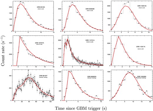
Background subtracted LCs of the GRBs in 8–900 keV energy range for the NaI detector in which the count rate is maximum. The upper six panels are ‘hard-to-soft’ pulses and the lower three panels are ‘intensity tracking’ pulses. The LCs are fitted with Norris’ exponential model (Norris et al. 2005). The corresponding values of this model are shown in Table 1.
2.2 Spectral analysis
GBM contains 12 NaI detectors, numbered as nx, where x runs from 0 to 11 (in hexadecimal system, i.e. n0 to n9 and then ‘na’ and ‘nb’, where ‘a’ stands for 10 and ‘b’ stands for 11), and two bismuth germanate (BGO) detectors, denoted similarly as by. The NaI detectors cover the lower energy part of the spectrum (8–900 keV), while the BGO covers 200 keV–40 MeV (Meegan et al. 2009). The data are supplied in three formats: (1) time tag events (TTE) – time and energy channel information as registered by the detector of the individual tagged event (both source and background events) are stored; (2) CSPEC: spectrum binned in 1.024 s (during the burst) and 4.090 s (before and after the burst), with full spectral resolution are stored and (3) CTIME: binned data in 0.064 s bins and eight energy channels are stored. We choose TTE data due to its high time resolution for time-resolved spectroscopy. We examine the quicklook products from the supplied data and choose three NaI detectors which have registered the highest count rate. We choose one of the BGO detectors – b0, if x ≤ 5 and b1, otherwise. For ambiguous cases, we choose one of the BGO detectors subject to where x occurs in most of the cases. For the background estimation, we choose regions before and after the burst, as long as possible, but away from the burst. We fit up to fourth-order polynomial to model the background, and interpolate the function to estimate the background during the burst.
For time-resolved study, we divide the duration of a GRB by requiring a minimum of 1200 background subtracted counts per time bin (i.e. 35σ) for the NaI detector having the highest count rate. We start to integrate the count from the zero flux level and integrate till this count is reached. The choice of required count per time bin is subjective. The choice depends on two competing perspectives: (i) finer time bin may give larger uncertainties in the parameters; (ii) wider time bin may not capture the evolution. We made the choice of the time intervals such that the variation may be comparable with the uncertainty. We found that this is the case when we use 0.5 s time bins at the peak. As these GRBs have ∼2500 count rate at the peak, 1200 count is a good choice. Note that Lu12 also have used the same σ level. Only in the case of GRB 100707A the requirement is 2500 count bin−1 (i.e. 50σ), as the count rate of this GRB is much higher than the rest. Note that due to lower effective area of BGO, it is not suitable for time-resolved spectroscopy (see e.g. Ghirlanda, Nava & Ghisellini 2010). The count in the BGO energy range is often less than 2σ. However, it is necessary to use this detector to constrain the high energy part of the spectrum. Hence, we use larger bin size for the spectrum in the BGO energy range, i.e. five or seven bins are used with progressively higher bin size at higher energy. Spectrum of NaI detectors is binned requiring 40 counts bin−1. We use rmfit v3.3pr7 for LC extraction and background estimation. The time-resolved spectral study is performed using xspec v12.6.0. We use χ2 minimization procedure to estimate the parameters and their nominal 90 per cent error. Note that the parameter estimation done by χ2 technique does not deviate larger than 10 per cent from the c-stat technique for a count of 1000 (see Nousek & Shue 1989). We have used χ2 technique to compare goodness of fit between different models which cannot be done for c-stat method. In Basak & Rao (2013a), we have conclusively shown for a set of GRBs that the deviation of parameter values due to different statistics (i.e. χ2 and c-stat) is smaller than that due to different choice of detectors, background time and modelling etc.
We use four models for time-resolved spectral fitting. These are (1) Band function, (2) blackbody along with a power law (BBPL), (3) a disc blackbody, having continuous temperature profile with radius, along with a power law (mBBPL) and (4) two blackbodies along with a power law (2BBPL). BR13 have used these models for the individual pulses of two GRBs, namely, GRB 081221 and GRB 090618.
3 RESULTS
3.1 Results of timing study
We fit the LCs of all the GRBs using equation (1). These are shown in Fig. 1. We note that Norris model adequately captures the pulse profile of all the GRBs. However, note that the |$\chi ^2_{\rm red}$| are generally not good. This is due to the fact that the pulses, other than the broad structure, have very rapid variations (see Rao et al. 2011). These finer time variabilities cannot be captured in a simple pulse structure. In the current study, we are interested to quantify broad pulse properties e.g. width and asymmetry of the pulses. Hence, the use of Norris model is adequate for our purpose.
In Table 1, we report the parameters of Norris model fit. The errors in the derived parameters are calculated by propagating the mean error of the Norris model parameters (see Norris et al. 2005). Uncertainty in p, however, is obtained by noting down the |$\chi ^2_{\rm red}$| for different values of p because the correlated errors in τ1 and τ2 give incorrect results, particularly for symmetric GRBs. The width (w) and asymmetry (κ), however, are well determined. Though these GRBs have broad single pulses, we find that for GRB 081207, which is a very long GRB compared to all others, at least two heavily overlapping pulses are present during the main bursting episode. Also, for GRB 110721A, we found that fitting two pulses is significantly better than a single pulse fitting (an improvement of Δχ2 = 205.1 is obtained to the expense of 4 degrees of freedom).
Parameters for Norris model fit to the LC of the GRB pulses. We also report the time interval (t1–t2) in which we have performed our analysis, number of time bins (n) within the time interval and the best detectors used for time-resolved spectroscopy.
| Specification of | ||||||||||
|---|---|---|---|---|---|---|---|---|---|---|
| GRB | Norris model parameters | time-resolved analysis | ||||||||
| ts (s) | τ1 (s) | τ2 (s) | |$\chi ^2_{\rm red}\ ({\rm dof})$| | p (s) | w (s) | κ | t1, t2 (s) | n | Detectors used | |
| 081224 | |$-1.53_{-0.26}^{+0.34}$| | |$3.60_{-1.07}^{+0.99}$| | |$3.30_{-0.21}^{+0.27}$| | 6.80 (13) | 1.90 ± 0.10 | 7.5 ± 0.7 | 0.44 ± 0.03 | −0.5, 19.6 | 15 | n6, n7, n9, b1 |
| 090809B | |$-1.74_{-0.38}^{+0.31}$| | |$9.35_{-1.85}^{+2.59}$| | |$2.50_{-0.17}^{+0.17}$| | 5.88 (13) | 3.10 ± 0.09 | 7.4 ± 0.6 | 0.34 ± 0.02 | −4.0, 19.3 | 15 | n3, n4, n5, b0 |
| 100612A | |$-8.43_{-2.65}^{+1.61}$| | |$156.4_{-57.4}^{+137.6}$| | |$0.88_{-0.17}^{+0.14}$| | 16.8 (9) | 3.30 ± 0.06 | 6.5 ± 1.5 | 0.14 ± 0.02 | −2.0, 17.2 | 11 | n3, n4, n8, b0 |
| 100707A | |$-2.5_{-2.6}^{+3.2}\times 10^{-2}$| | |$0.37_{-0.05}^{+0.04}$| | |$7.19_{-0.16}^{+0.18}$| | 4.01 (233) | 1.60 ± 0.07 | 9.9 ± 0.28 | 0.72 ± 0.01 | −1.0, 22.6 | 18 | n4, n7, n8, b1 |
| 110721A | |$-0.62_{-0.15}^{+0.08}$| | |$1.58_{-0.46}^{+0.67}$| | |$1.59_{-0.23}^{+0.15}$| | 1.32 (229) | 0.96 ± 0.10 | 3.55 ± 0.62 | 0.45 ± 0.03 | −1.0, 10.6 | 15 | n6, n7, n9, b1 |
| |$1.75_{-0.07}^{+0.10}$| | |$0.079_{-0.053}^{+0.074}$| | |$6.75_{-0.66}^{+0.86}$| | 2.48 ± 0.12 | 8.08 ± 1.04 | 0.83 ± 0.05 | |||||
| 110817A | |$-0.62_{-0.42}^{+0.30}$| | |$1.11_{-0.66}^{+1.31}$| | |$1.76_{-0.24}^{+0.24}$| | 1.85 (8) | 0.78 ± 0.12 | 3.6 ± 0.8 | 0.49 ± 0.08 | −0.3, 7.1 | 8 | n6, n7, n9, b1 |
| 081207 | |$-8.55_{-2.21}^{+3.30}$| | |$14.14_{-6.10}^{+9.10}$| | |$50.79_{-10.22}^{+11.10}$| | 1.36 (114) | 18.25 ± 3.36 | 90 ± 21 | 0.57 ± 0.06 | −7.0, 76.0 | 20 | n1, n9, na, b1 |
| −9.64 | 304.7 | |$9.24_{-2.20}^{+3.50}$| | 43.42 ± 1.19 | 45 | 0.20 | |||||
| 090922A | |$-0.39_{-0.19}^{+0.15}$| | |$0.62_{-0.27}^{+0.38}$| | |$4.00_{-0.30}^{+0.30}$| | 6.23 (15) | 1.18 ± 0.18 | 6.4 ± 0.7 | 0.62 ± 0.05 | −4.0, 13.4 | 8 | n0, n6, n9, b1 |
| 100528A | |$-32.6_{-2.36}^{+2.36}$| | |$1262.0_{-61.1}^{+60.9}$| | |$1.29_{-0.38}^{+0.14}$| | 6.56 (21) | 7.70 ± 0.06 | 14.5 ± 3.0 | 0.09 ± 0.004 | −3.0, 21.4 | 16 | n6, n7, n9, b1 |
Lu12 have suggested that the HTS pulses are more asymmetric than the IT pulses. However, from Table 1 we find that there are some exceptions to this consensus for our single pulse sample. For example, GRB 100612A, which is a HTS GRB, is very symmetric (κ is only 0.14 ± 0.02). GRB 090922A, despite being an IT GRB, is very asymmetric (as high as 0.62 ± 0.05). The highest asymmetry is shown by single pulse GRB 100707A. We visually inspect this GRB and find that the rising part is in fact very steep. Hence, in order to get more data point in the rising part, we analyse the LC using 0.1 s bin size. We find the asymmetry, κ = 0.72 ± 0.01, which is indeed the highest among all the GRBs. Though we found two pulses in GRB 110721A, one of these pulses shows even higher asymmetry κ = 0.83 ± 0.05. One of the two pulses of GRB 081207, an IT GRB, show high asymmetry (0.57 ± 0.06). Hence, we cannot differentiate between HTS and IT GRBs according to their asymmetric LCs.
3.2 Results of time-resolved spectroscopy
As described in Section 2.2, we extract the time-resolved spectra of the individual GRBs by requiring a minimum background subtracted count per time bin. The time interval (t1–t2) and the number of bins (n) are listed in Table 1. For GRB 081207, which has another pulse after 80 s, the data are taken till 76 s. This selection, however, will not affect any conclusion regarding this GRB. We also report the detectors used in our analysis in the last column of Table 1.
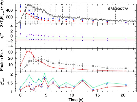
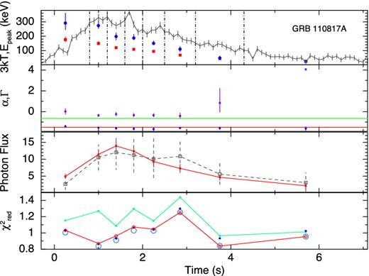
The results of the time-resolved spectroscopy for all the GRBs are shown graphically in Figs 2 –10. The upper panels show the kT variation of the BBPL and Epeak variation of the Band function. We have shown the LCs of the individual GRBs in this panel to compare the Epeak variation with the count rate variation. From this variation we can identify that the first six GRBs are the HTS GRBs and the rest three are IT GRBs. Note that the peak of BB occurs at ∼3kT, and hence, in this panel, we have plotted 3kT instead of kT to compare the peak position given by the BBPL and Band function fit. We note that there is a general agreement of evolution of these peaks, however, the peak of the BBPL fit is always found to be lower than the corresponding νFν peak of the Band function.
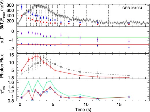
GRB 081224. From upper panel, panel 1: variation of 3 kT (red filled boxes) and Epeak (blue filled circles) with time. Shown in background is the corresponding LC plotted in the same scale as in Fig. 1. The dot–dashed lines denote the time intervals used for spectral analysis. The parameters are shown at the mean time of each interval. Panel 2: α (violate boxes) of Band function and Γ (blue circles) of BBPL model. The lines denote the synchrotron ‘lines of death’ (one at −3/2 and another at −2/3). Panel 3: flux (photons cm−2 s−1) variation of BB (filled boxes joined by straight lines) and PL (open boxes joined by dashed line). The PL flux is scaled by the ratio of total BB flux and total PL flux. Panel 4: |$\chi ^{\rm 2}_{\rm red}$| for BBPL (green filled boxes), Band (red open circles), mBBPL (blue filled circles) and 2BBPL (largest open circles).
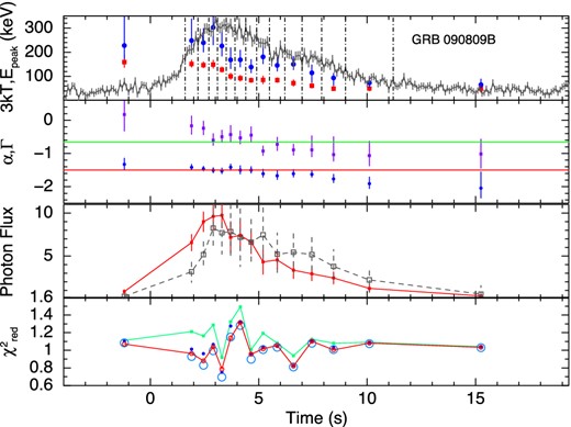
GRB 090809B. Symbols used are the same as in Fig. 2.
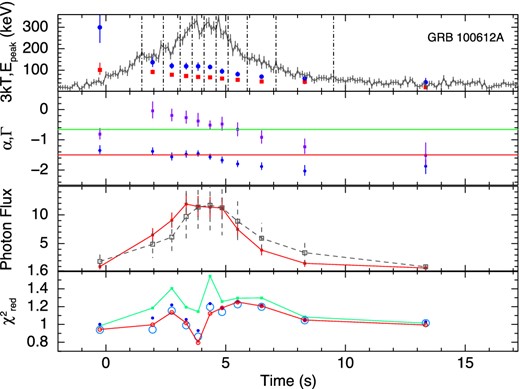
GRB 100612A. Symbols used are the same as in Fig. 2.
GRB 100707A. Symbols used are the same as in Fig. 2.
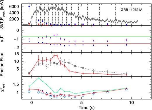
GRB 110721A. Symbols used are the same as in Fig. 2.
GRB 110817A. Symbols used are the same as in Fig. 2.
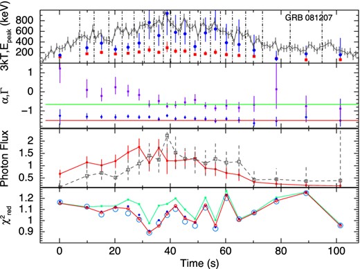
GRB 081207. Symbols used are the same as in Fig. 2.
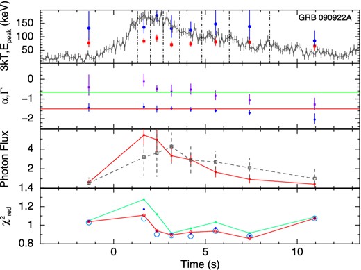
GRB 090922A. Symbols used are the same as in Fig. 2.
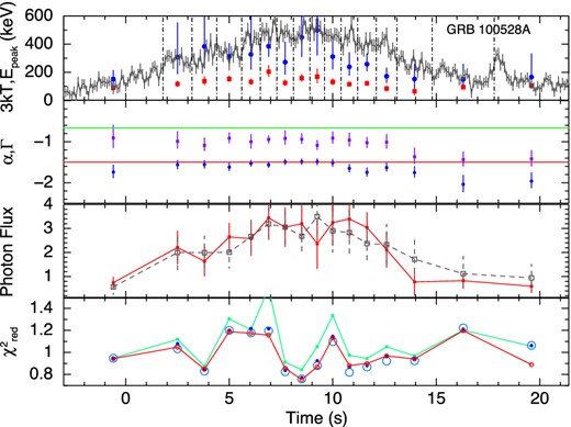
GRB 100528A. Symbols used are the same as in Fig. 2.
In the second panels from the top, we have shown the variation of α of the Band function and Γ of the BBPL model. The parameter β is often unconstrained or reaches the hard bound of −10. Hence, we do not show this parameter. In this panel, we show the ‘synchrotron lines of death’ by two straight lines – one at −2/3 (slow cooling regime) and another at −3/2 (fast cooling regime). The general trend of α is higher at the beginning and lower in the later part. Note that the value α is always greater than the line at fast cooling regime (−3/2). To quantify the deviation of α from the predicted −3/2 line, we device two methods: (a) the deviation of the mean value of α from −3/2 in the units of σ and (b) the χ2 value of the fit to α, assuming the model predicted α = −3/2. In Table 2 (column 4), we have shown the mean values of α for each GRB. The error in the mean is 1σ, and it is calculated by using the two tailed errors of α (at nominal 90 per cent confidence). The deviation of the mean from −3/2 value in the units of σ is shown in column 5. We see a high deviation in each case. The |$\chi ^2_{\rm red}$| (shown in parenthesis) is also high in each case denoting the significance of the trend. In some cases, its value is greater than −2/3, which is disallowed by synchrotron model for slow cooling electrons. This deviation from −2/3 line, however, is not very significant. For some HTS GRBs the deviations are significant: 40σ (GRB 100707A), 5.8σ (GRB 081224) and 5.0σ (GRB 110817A). For IT GRBs the deviations are consistent with zero (within 1σ). For IT GRB 100528A, the mean value of α is −1.02 ± 0.04 which is even within the slow cooling ‘line of death’ at 8.8σ. We find two extreme cases. These are GRB 110817A (HTS) and GRB 100528A (IT). In the former case, α values are always above the line at −2/3 and in the latter case α values are always below the line.
Classification of the GRBs: hard-to-soft (HTS) and intensity tracking (IT) based on the spectral analysis.
| GRB | Type | Behaviour of | Mean α | Deviation of α a | α crossing −2/3 | Band/BBPLb | LAT detection |
|---|---|---|---|---|---|---|---|
| the PL flux | from −3/2 (|$\chi ^2_{\rm red}$|) | ‘line of death’ | |||||
| 081224 | HTS | Clear delay and lingering | −0.43 ± 0.04 | 26.7σ (53.5) | 11/15 | 0.80 (0.14) | 3.1σ |
| 090809B | HTS | Mild delay and lingering | −0.64 ± 0.06 | 14.3σ (13.5) | 8/15 | 0.74 (0.15) | No |
| 100612A | HTS | Very mild lingering | −0.58 ± 0.07 | 13.1σ (19.1) | 7/11 | 0.73 (0.15) | No |
| 100707A | HTS | Clear delay and lingering | 0.013 ± 0.017 | 89.0σ (71.6) | 16/18 | 0.74 (0.23) | 3.7σ |
| 110721A | HTS | Clear delay and lingering | −0.95 ± 0.02 | 27.5σ (56.2) | 2/15 | 0.94 (0.10) | 30.0σ |
| 110817A | HTS | Mild lingering | −0.31 ± 0.07 | 16.9σ (34.1) | 8/8 | 0.81 (0.09) | No |
| 081207 | IT | Mild delay | −0.63 ± 0.06 | 14.5σ (10.5) | 10/20 | 0.66 (0.12) | No |
| 090922A | IT | Mild delay and lingering | −0.66 ± 0.10 | 8.4σ (9.7) | 5/8 | 0.67 (0.13) | No |
| 100528A | IT | Mild lingering | −1.02 ± 0.04 | 12.0σ (9.8) | 0/16 | 0.68 (0.14) | No |
aDeviation of the mean value of α from the −3/2 ‘line of death’ (fast cooling) in the units of σ is shown. |$\chi ^2_{\rm red}$| is the reduced χ2 of the fit of α values assuming the model α = −3/2. Higher |$\chi ^2_{\rm red}$| denotes higher deviation from the synchrotron model predicted photon index (for fast cooling).
bBand function compared to the BBPL model. F-test is performed to check the superiority of Band function over the BBPL model for all the time-resolved spectrum of each GRB. The reported values are the mean (and standard deviation) of the confidence level of F-test.
In the third panels, we have shown the evolution of the photon flux for the two components of BBPL model. Note that the PL flux lags behind the BB flux. This behaviour is particularly significant for GRB 081224, GRB 100707A and GRB 110721A. In a recent paper, Basak & Rao (2013b) have shown that very high energy (GeV) emission is expected for GRBs which have delayed PL emission. For the three GRBs in the present study, we also find reported Large Area Telescope (LAT) detection [Low-Energy Event (LLE) data] at 3.1σ, 3.7σ and 30.0σ, respectively (Ackermann et al. 2013). Though we have not used the LAT data of these GRBs for spectroscopy, the LAT detection is consistent with our earlier claim.
Finally, the fourth panels show the |$\chi ^2_{\rm red}$| of various model fits. To compare the fit statistics of BBPL model with other models, we perform F-test between BBPL and Band function. The confidence level (CL) that the alternative model (Band) is better than the original hypothesis (BBPL) is calculated for all the time-resolved bins of the individual GRBs. We then compute the mean and standard deviation of the CL. The corresponding values are reported in Table 2. It is evident that the IT pulses are adequately fit by BBPL model. The HTS pulses, on the other hand, require a different model to fit the spectrum. However, Band, mBBPL and 2BBPL are all equally good for this purpose. Hence, one needs physical arguments to distinguish between these models.
The results of all the GRBs are summarized in Table 2. We note that the GRBs can be classified in two categories: HTS and IT. We note the following trends for HTS and IT GRBs. First, note that a LAT detection is reported only for HTS class. For HTS GRBs, the value of α is greater than −2/3 in 63.4 per cent cases. The exception of this trend is shown by GRB 110721A. Excluding this GRB, we obtain 74.6 per cent of cases of HTS GRBs where α is greater than −2/3. The deviation of α from −3/2 line is systematically high (large σ deviation and high values of |$\chi ^2_{\rm red}$|). The confidence level (CL) that the Band model is better than the BBPL model has a mean value of 79.3 per cent. In the case of IT GRBs, the value of α is greater than −2/3 in only 44 per cent cases. As pointed out the mean values are greater only within 1σ deviation, and for one IT GRB (namely, 100528A) it is even less than −2/3 at 8.8σ. Also, the CL that the Band model is better than BBPL model has a mean value of only 67 per cent. The only exception of the behaviour of α is noted for the HTS GRB 090809B for which α is greater than −2/3 in only 53.3 per cent cases. However, note in Fig. 3 (upper panel) that the Epeak evolution is not strictly hard-to-soft. In Fig. 11 (left-hand panel), we have plotted the α values for HTS and IT GRBs, with y-axis as time sequence. In the same plot, we have indicated the −3/2 and −2/3 lines of death. Note that α values are always greater than the −3/2 line. In many cases the α values are greater than the −2/3 line, especially for the HTS GRBs. The mean value of α is −0.42 and −0.68 for HTS and IT GRBs with dispersion of 0.72 and 0.50, respectively. Also there is a clear trend of the evolution of α – the values of α decreases with time, i.e. the spectrum becomes softer.
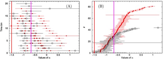
(A) The values of α for all GRBs – filled circles for HTS class and open boxes for the IT class. The errors are calculated at nominal 90 per cent confidence. The y-axis denotes the time bin from start to end. The thick red and purple lines are the lines of death at α = −3/2 and −2/3, respectively. (B) Same as (A), with values of α sorted in ascending order. The values of α are always greater than −3/2 (see Table 2 for significance). Note that the region of α < −2/3 (i.e. the left of the purple line) is mainly populated by IT GRBs, while the α values of HTS GRBs appear in the region of α > −2/3. The mean value of α are −0.42 and −0.68 for HTS and IT GRBs, respectively.
4 DISCUSSION
4.1 Features of 2BBPL model
The four models used in our analysis are taken from BR13, who applied them to the brightest GRBs having separable pulses (GRB 081221 and GRB 090618). The present results generally agree with the results obtained for those two bright GRBs. In the present case too we find that the decomposition of the spectrum in terms of 2BBs or mBB and a PL component significantly improves the fit over single BB with a PL. Though the 2BBPL model gives better |$\chi ^2_{\rm red}$| in all cases, the present analysis cannot conclusively show whether the 2BBPL model is an approximation for some underlying complex spectral distribution. Exploring this model further, Basak & Rao (2013b) have shown some very promising results like prediction of LAT emission from GBM only analysis. They have fitted the MeV GBM data, without invoking the LAT data, with the 2BBPL model and have shown that the PL flux, independent of the LAT data, mimics the LAT GeV emission. The PL has a delayed onset and lingers at the later part, just as the same way as the LAT flux. Moreover, the PL fluence correlates with the LAT fluence. In the present analysis, we find LAT detection for three GRBs (GRB 081224, GRB 100707A and GRB 110721A) which show similar behaviour (a delayed onset of the PL component which lingers at the later phase). Another interesting feature we find that the 2BBs of the 2BBPL model are highly correlated. In Fig. 12, we have plotted the temperatures of the two BBs of the 2BBPL model. It is clear that the two temperatures are highly correlated. This correlation shows that either there is some underlying physical reason for the two BB components or they are connected to each other because they happen to be an approximation for some more complex spectral shape.
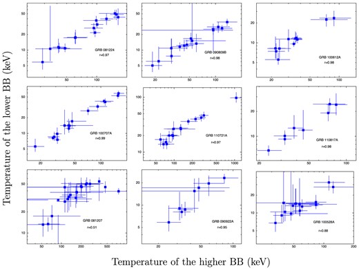
Correlation between the temperatures of the two BBs of 2BBPL model. The upper six panels are for HTS GRBs and the other three panels are for IT GRBs. We note significant correlation in all the cases.
5 SUMMARY
To summarize, we have collected a sample of GBM GRBs having single pulse. We have studied the individual pulses in the time and energy domain and found some interesting results. We found that the Band model always gives better fit to the data compared to the BBPL model. The |$\chi ^2_{\rm red}$| of the Band model is comparable to mBBPL and 2BBPL model. However, the values of α, in many cases, are greater than −2/3, the limit due to the synchrotron emission from electrons in the slow cooling regime. Hence, the spectrum cannot be fully synchrotron. Hence, neither BBPL nor Band can be considered consistent with the underlying physical mechanism of the prompt emission. It is possible that both thermal and non-thermal emissions contribute to the total emission. In this regard, the 2BBPL and the mBBPL model are preferred over BBPL model. We found that the HTS GRBs have generally larger values of α compared to the IT GRBs. Also, the α has a decreasing trend with time, making the spectrum softer. This signifies that the spectrum has a different origin than synchrotron at the beginning, but later synchrotron emission may dominate.
We found that the peak energy of the BBPL model gives lower value than the corresponding Band function. As the peak energy of the spectrum is used for the correlation studies in the prompt emission (Amati et al. 2002; Ghirlanda, Ghisellini & Lazzati 2004; Yonetoku et al. 2004; Basak & Rao 2012b), it is essential to determine the correct peak energy of the spectrum. If the underlying reason for the Epeak and isotropic equivalent energy correlation (Epeak–Eγ, iso: the Amati correlation) is some basic physical process, a correct model description and a proper identification of Epeak would be required to improve the Amati-type correlation (note that Epeak and 3 kT are not strictly correlated with each other and the difference varies between GRBs). Investigating a pulse-wise Amati correlation (e.g. see Krimm et al. 2009; Basak & Rao 2013c) with different models to derive the Epeak can provide inputs to strengthen the Amati correlation as well as to identify the physical process responsible for the correlation. Note that a HTS evolution, by its nature violate time-resolved Epeak–Eγ, iso correlation, because the high values of Epeak is obtained even when the flux (and hence Eγ, iso) is low. For example, Axelsson et al. (2012) have found Epeak ∼ 15 MeV during the initial bins of GRB 110721A. Hence, time-resolved Amati correlation is likely to fail. Basak & Rao (2012a) have studied Amati correlation by replacing time-resolved Epeak and Eγ, iso by pulse average Epeak and total Eγ, iso of a pulse. A pulse average Epeak, due to the crucial averaging over a pulse, will not show the effect of HTS evolution history, thus restoring the Amati correlation. Note that pulses, rather than time-resolved bins are preferred as the pulses behave as independent entities in GRBs. In this context one reasonable choice is peak energy at the zero fluence (Epeak, 0) as done by Basak & Rao (2012a). Unlike Epeak, which is a pulse average quantity, Epeak, 0 is a constant for each pulse and correlates better with the total Eγ, iso. Consequently, the strong pulse-wise Epeak, 0–Eγ, iso correlation indicates that a pulse with high initial peak energy may have started with a low flux, but eventually it will give rise to high total flux of the pulse. However, one cannot use the IT class for such correlation study, as IT GRBs, by their nature will not give such Epeak, 0. Hence, one can use pulse average peak energy for such correlation study, which does not depend on HTS or IT evolution (Basak & Rao 2013c)
Finally, we want to remind that the 2BBPL model has some interesting features like highly correlated BB temperatures. The PL component of this model fitted to the prompt keV–MeV emission has been shown to correlate with the high-energy GeV emission (Basak & Rao 2013b). These definitely point towards some underlying physical process. Hence, it is important to find the existence of the 2BBs in the prompt emission spectrum. Making similar spectral analysis for GRBs with better low energy measurement [like that from Swift/X-Ray Telescope (XRT)] would clarify these further. As the temperature of the two correlated BBs decreases with time, the lower BB may show up in the low energy detector like XRT during the late prompt emission phase. However, such detailed study needs good knowledge of detector systematics and cross-detector calibration. In Basak & Rao (2012a), we have shown that spectral analysis using BAT and GBM gives systematics difference in the results. Though one needs to find out ways to perform joint fitting, the procedure is quite involved and beyond the scope of the present paper.
This research has made use of data obtained through the HEASARC Online Service, provided by the NASA/GSFC, in support of NASA High Energy Astrophysics Programs. We thank the referee for valuable comments and numerous suggestions especially to make quantitative statements of the results.
