


Abstract
We propose that the accretion of a dwarf spheroidal galaxy provides a common origin for the giant southern stream and the warp of M31. We run about 40 full N-body simulations with live M31, infalling galaxies with varying masses and density profiles, and cosmologically plausible initial orbital parameters. Good agreement with a full range of observational data is obtained for a model in which a dark-matter-rich dwarf spheroidal, whose trajectory lies on the thin plane of corotating satellites of M31, is accreted from its turnaround radius of about 200 kpc into M31 at approximately 3 Gyr ago. The satellite is disrupted as it orbits in the potential well of the galaxy and forms the giant stream and in return heats and warps the disc of M31. We show that our cosmologically motivated model is favoured by the kinematic data over the empirical models in which the satellite starts its infall from a close distance of M31. Our model predicts that the remnant of the disrupted satellite resides in the region of the north-eastern shelf of M31. The results here suggest that the surviving satellites of M31 that orbit on the same thin plane, as the disrupted satellite once did, could have all been accreted from an intergalactic filament.
1 INTRODUCTION
A significant fraction of observed galaxies exhibit tidal features such as tidal tails, streams and shells (Malin & Carter 1980, 1983). These features are widely believed to be the products of merger events (Hernquist & Quinn 1988, 1989). Numerous simulations have shown that tidal structures form during mergers of galaxies and observations of tidal structures have been used to put bound on various parameters, such as the orbital parameters and the masses of the host galaxies and their satellites.
In this work, we consider Andromeda or Messier 31 (M31) which is a rare example of a spiral galaxy that exhibits tidal features, such as streams and shells. Andromeda galaxy contains two rings of star formation off-centred from the nucleus (Block et al. 2006, and references therein) and most notably a Giant Southern Stream (GSS; Ibata et al. 2001, 2005, 2007; Ferguson et al. 2002; Bellazzini et al. 2003; Zucker et al. 2004; Brown et al. 2006; Richardson et al. 2008; McConnachie et al. 2009). The GSS is a faint stellar tail located at the southeast part of M31. It extends radially outward of the central region of M31 for approximately 5°, corresponding to a projected radius of ∼68 kpc on the sky. The stream luminosity is LGSS ∼ 3.4 × 10⁷ L⊙ corresponding to a stellar mass of MGSS ∼ 2.4 × 10⁸ M⊙ for a mass-to-light ratio of 7 (Ibata et al. 2001; Fardal et al. 2006).
In the follow-up observations of the GSS, two other structures corresponding to stellar overdensities, which are now believed to be two shells, have been discovered (Ferguson et al. 2002; Fardal et al. 2007; Tanaka et al. 2010; Fardal et al. 2012). The colour–magnitude diagram of the north-eastern (NE) shelf is similar to that of the GSS (Ferguson et al. 2005; Richardson et al. 2008). This similarity has been a strong argument in favour of models which predict that both the GSS and the NE are the results of a single merger event between M31 and a satellite galaxy (Ibata et al. 2004; Font et al. 2006; Fardal et al. 2007).
A major merger scenario, dating back to a few Gyr, from which M31, its giant stream, and many of its dwarf galaxies emerge has been proposed (Hammer et al. 2010, 2013). On the other hand, an empirical minor merger scenario has also been studied extensively, in which a satellite galaxy falls on to M31, from a distance of a few tens of kpc, on a highly radial orbit (of pericentre of a few kpc) less than one billion year ago. The satellite is tidally disrupted at the pericentre passage and forms the observed M31 stream and the two shelves (Fardal et al. 2006, 2007). Although these empirical models provide good fits to the observations, they suffer from simplifications. First, M31 is not modelled as a live galaxy but is only presented by a static potential and consequently the effect of dynamical friction (DF) is not properly taken into account. Secondly, there is no dark matter in the progenitor satellite whereas a good fraction of satellite galaxies in the Local Group seem to be dark matter rich. Finally, the origin of the infalling satellite and its trajectory in the past is completely overlooked. It is highly implausible that a satellite on a highly radial orbit could have survived to arrive at an easy reach of M31.
In this work, we run full N-body simulations of mergers of satellites with a live M31. We take M31 as a live galaxy composing of a disc, a bulge and a dark matter halo of varying mass-to-light ratios and study the infalls of satellites with different density profiles, masses and orbital parameters. Although a live realization of M31 has already been simulated for this model to derive an upper limit on the mass of the satellite (see e.g. Mori & Rich 2008), here we study the dependence of the properties of the simulated stream on the internal structures of the progenitor and also study the history of the satellite itself. First, we confirm that the empirical models, in which a dark-matter-poor satellite falls on a highly radial orbit from a short distance of a few tens of kiloparsecs, reproduce various observed features of the giant stream of M31. We study the orbital history of the satellite back in time and show that it is expected to have experienced several close encounters with M31 (Ibata et al. 2004; Font et al. 2006). We demonstrate that a satellite that survives to reach within a short distance of its host halo is unlikely to have followed a highly eccentric orbit.
We propose an alternative cosmologically plausible scenario for the origin of the giant stream and also the warp structure of M31 disc itself. Here, a dark-matter-rich satellite is accreted and falls from its first turnaround radius, on an eccentric orbit on to M31. The best agreement with the observational data is obtained when the satellite lies on the same plane that contains many of the present dwarfs of M31 (Conn et al. 2013; Ibata et al. 2013). Unlike previous empirical models, the disc of M31 is perturbed by the infall of the massive satellite in our model and becomes warped.
The paper is organized as follows. In Section 2, we present details of our numerical simulations and N-body modelling. In Section 3, we present results for the empirical models of GSS formation. Section 4 is devoted to the study of the orbital history of the satellite. In Section 5, we present the results for our alternative ‘first-infall’ scenario. The perturbation, heating and warping of the disc of M31 due to the infall of the satellite are discussed in Section 6. We conclude in Section 7.
2 NUMERICAL METHODS
2.1 M31 mass model
The large spiral galaxy M31, at a distance of d = 785 ± 25 kpc from Milky Way, is probably the most massive, with a mass of M300 = 1.4 ± 0.4 × 10¹² M⊙ (Watkins, Evans & An 2010), member of the Local Group.
Values of the parameters for different components of M31, used in our simulations.
| Component | Model | Scalelength(s) | Mass | Additional parameters |
|---|---|---|---|---|
| (kpc) | (1010 M⊙) | |||
| Disc | Exponential disc | Radial: Rd = 5.40 | 3.66 | |
| Vertical: z0 = 0.60 | ||||
| Bulge | Hernquist sphere | 0.61 | 3.24 | |
| Halo | NFW sphere | 7.63 | M200 = 88 | c = 25.5 |
| r200 = 195 kpc |
To generate the N-body realization of M31, we use the technique developed in previous works (Hernquist 1993; Springel & White 1999) which consists of approximating the velocity distribution by a three-dimensional Gaussian whose moments are calculated using Jeans’ equations. The halo of M31 is represented by N = 241 369 particles while the bulge and the disc have N = 96 247 and 108 929, respectively. This ensures that the mass resolution for dark matter is, at most, 10 times the mass resolution for the baryons, as given in Table 2.
Number of particles and mass resolution for our N-body realization of M31.
| Component | N | m (M⊙) |
|---|---|---|
| Disc | 108 929 | 3.36 × 10⁵ |
| Bulge | 96 247 | 3.36 × 10⁵ |
| Halo | 241 369 | 3.36 × 10⁶ |
| Component | N | m (M⊙) |
|---|---|---|
| Disc | 108 929 | 3.36 × 10⁵ |
| Bulge | 96 247 | 3.36 × 10⁵ |
| Halo | 241 369 | 3.36 × 10⁶ |
2.2 The satellite progenitor
2.2.1 Morphology
Based on the mass of the giant stream, which is found to be around 2.4 × 10⁸ M⊙, and the extent of the giant stream, the stellar mass of the progenitor satellite has been estimated to be around M = 2.2 × 10⁹ M⊙ (Font et al. 2006; Fardal et al. 2007). However, the morphology and the density profile of the progenitor are not immediately constrained by the giant stream and the shelves. Consequently, we have run simulations with different profiles and components. In total we ran about 40 simulations, by varying the density profile, dark matter content and the initial orbital parameters of the satellite. We point out that our simulations are purely dissipationless and do not treat any gaseous component that may have been present in the satellite. We also do not include stellar population modelling or some recipe for star formation as it is beyond the scope of our study which focuses mainly on the dynamics of the interaction. We group our simulations into two categories. The first category of the simulations uses a satellite with no dark matter and the common best-fitting values of the orbital parameters (Fardal et al. 2007, 2013). We shall refer to these models as the empirical models. The simulation results for this category of models are presented in Section 3. In the second set of simulations, we search in different parts of parameter space for models with a dark-matter-rich satellite and use cosmologically motivated initial orbital parameters. The results corresponding to this category of models are presented and discussed in Section 5.
For each category of models, we run simulations with two different morphologies for the satellite: first we assume that the satellite was a hot spheroid and run a simulation with a Plummer profile of scale radius a = 1.03 kpc. It has already been reported that a satellite with such a profile satisfactorily reproduces the observed properties of the giant stream (Fardal et al. 2007, 2013). The difference with the previous works is that here we have a live M31 and consequently can properly take into account the effect of DF. We shall refer to this as the Plummer model or shortly Plummer. We also run two further simulations with spherical Hernquist profiles, one with same scale radius a = 1.03 kpc as the Plummer model and one with a = 0.55 kpc, the latter is chosen such that the half-mass radius of the Hernquist model is equal to that of the Plummer model. We shall refer to these models as Hernquist1 and Hernquist2.
In a second set of runs, we assume that the satellite was a cold rotating disc, which seems to reproduce the second-order properties of the giant stream, in particular the observed asymmetry in the transverse density profile, even better than the previous examples of hot spheroids (McConnachie et al. 2003; Gilbert et al. 2007; Fardal et al. 2008). We use a two-component model for the progenitor consisting of an exponential (sech2) disc as given by equation (2), with a mass of Md = 1.8 × 10⁹ M⊙, a scale radius of Rd = 0.8 kpc and a vertical scalelength zd = 0.4 kpc, as well as a Hernquist bulge of mass Mb = 0.4 × 10⁹M⊙ and scale radius 0.4 kpc. Because we lack constraint on the orientation of the disc, we consider six different models with evenly spaced values of the inclination and position angles, Ax and Az, respectively. We refer to these disc models as Disci with i = 1 , …, 6.
2.2.2 N-body realization: nbodygen
The equilibrium N-body realizations of the progenitor satellites is generated by our code, nbodygen, which is specially tailored for the Plummer, Hernquist1 and Hernquist2 models.
nbodygen is a code used to generate N-body realizations of multicomponent elliptical and spheroidal galaxies with an optional central black hole.1 The positions of particles for each component (bulge and halo) are selected by sampling the cumulative mass profile. The velocities are sampled from the self-consistent distribution function given by Eddington's formula (see e.g. Binney & Tremaine 1987; Kazantzidis, Magorrian & Moore 2004). The integrand in Eddington's formula is tabulated on a grid uniformly spaced in x = r/(r + rs) where rs is a characteristic radius of the profile. The distribution function is then calculated numerically on a grid of relative energy ϵ and linear interpolation is used whenever needed to obtain values other than the tabulated ones.
For the spherical Plummer and Hernquist profiles, we run our simulations with a total number of N = 131 072 particles to model the progenitor satellite. The disc progenitors are initialized using the same method as that used in the previous subsection to make the N-body realization of M31. In the case of disc models, the number of particles in the disc is set to N = 107 143 and in the bulge to N = 23 809 in order to have the same particle mass resolution in both components. Given the chosen values for the number of particles and the progenitor mass, the particle mass in all models is ms = 1.68 × 10⁴ M⊙ (Table 3). The softening length is set to ε = 30 pc for the satellite while it is ε = 39 pc for the baryonic component and ε = 390 pc for the halo of M31.
Values of parameters for different progenitor satellites used for an empirical modelling of the giant stream with live M31. The inclination angle Ax and the position angle Az are of the satellite w.r.t. the disc of M31.
| Model | Profile | Mass | Scale radius | Ax | Az | N | m |
|---|---|---|---|---|---|---|---|
| (109 M⊙) | (kpc) | (°) | (°) | M⊙ | |||
| Spherical | |||||||
| Plummer | Plummer | 2.2 | 1.03 | 131 072 | 1.68 × 10⁴ | ||
| Hernquist1 | Hernquist | 2.2 | 1.03 | 131 072 | 1.68 × 10⁴ | ||
| Hernquist2 | Hernquist | 2.2 | 0.55 | 131 072 | 1.68 × 10⁴ | ||
| Disc | |||||||
| Disc1 | Exponential | Disc = 1.8 | Rd = 0.8, zd = 0.4 | 0 | 0 | 107 143 | 1.68 × 10⁴ |
| Hernquist | Bulge = 0.4 | rb = 0.4 | 23 809 | 1.68 × 10⁴ | |||
| Disc2 | – | – | – | 45 | 0 | – | – |
| Disc3 | – | – | – | 45 | 45 | – | – |
| Disc4 | – | – | – | 45 | 90 | – | – |
| Disc5 | – | – | – | 90 | 0 | – | – |
| Disc6 | – | – | – | 90 | 45 | – | – |
3 EMPIRICAL MODELLING OF THE M31 GIANT STREAM
3.1 The orbital parameters
3.2 Identification of tidal structures
The total simulation times correspond to a few orbital periods and we analyse the results at a time step that would yield the best agreement between the simulated stream and the observed stream and shelves. More precisely, we compare consecutive simulation snapshots after the first pericentric passage of the satellite leading to the formation of the stream and select the one that matches best the different observables. For the empirical models, this corresponds to a time T ∼ 840 Myr after the start of the simulation. Fig. 1 shows the resulting real and phase-space projection for a satellite initialized with a Plummer profile. Particles are coloured by the numbers of pericentric passages that they experience during the run. We use the phase-space plot to identify the shelves and the stream. The Giant stream is easily identified and constitutes mostly of stars with negative velocity with respect to M31. Its spatial extension can also be directly estimated from the phase-space plot and is ∼140 kpc consistent with the observed value of 125 kpc (Ibata et al. 2004). The shelves manifest themselves as zero velocity surfaces in phase space and hence are easily identified in a phase plot. Three of these phase structures can be found in Fig. 1 and two of them are associated with the NE and western (W) shelves. The third inner caustic has not yet been observed but is clearly a prediction of this model. The phase-space projection also clearly reveals that each tidal structure is formed of particles that went through equal numbers of pericentric passages. Thus, the tidal structures are formed by particles with similar initial orbital energies that have been stripped from the satellite.
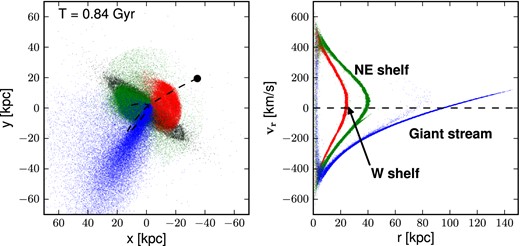
Real space x-y (left-hand panel) and phase-space r-vr (right-hand panel) projection of stellar particles in the progenitor satellite with a Plummer profile at the final time, t = 0.84 Gyr. On the x-y projection, we also show the particles that compose the disc of M31 (black dots) and the orbit of the progenitor (dashed line) as traced by the initially-most-tightly-bound particles. In both panels, the particles of the progenitor are colour-coded by the number of their pericentric passages: 1 (blue), 2 (green) or 3 (red).
3.3 Spatial extent, morphology and stellar mass
Next, we make a more detailed comparison with the observations. Fig. 2 shows the stellar density maps in standard sky coordinates at T = 840 Myr for the three models using a dynamically hot satellite with a spherical density profile, namely the fiducial Plummer model and the two Hernquist models (Hernquist1 and Hernquist2). The fields covering the spatial region occupied by the GSS and which have been used for the follow-up observations (McConnachie et al. 2003; Ibata et al. 2004) are plotted as solid rectangles with proper scaling on this figure.
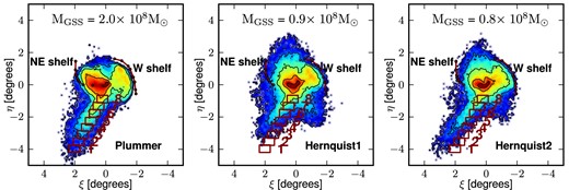
Spherical progenitors: stellar density maps in standard sky coordinates corresponding to particles of the satellite for the three different spherical models; Plummer, Hernquist1 and Hernquist2 (from left to right). The position of the observed stream fields from McConnachie et al. (2003) is overplotted with the size of the field of view of the CFH12k camera. The solid lines indicate the observed edges of the shelves. The total masses MGSS of particles which are selected as stream members in each of our N-body models are indicated on each panel. Clearly, the satellites initialized with a cuspy Hernquist profile provide an overall poorer fit (for both position and stream mass) to the data than a core Plummer profile.
For the Plummer model (left-hand panel), we clearly see that the simulated stream is in good agreement with the observations regarding the morphology and spatial extent of the giant stream. The total mass Mstream in the simulated stream can be calculated once the particles which did not originally belong to the satellite have been removed. We find Mstream = 2 × 10⁸ M⊙ in excellent agreement with the value of 2.4 × 10⁸M⊙ derived from observations. We can also compare the spatial distribution of satellite particles with the positions of the edges of the shelves. These edges are indicated as solid lines in Fig. 2 which are drawn by joining the data points (Fardal et al. 2007). We can see that there is still a fairly good agreement between the N-body model and the observation. In particular, the azimuthal and radial extent of the shelves are approximately reproduced with a better agreement for the W shelf.
The Hernquist models do not succeed in reproducing correctly the proper apparent direction of the GSS on the sky. The deviations between the direction of the simulated and observed streams are not dramatic (a few degrees) but still indicate clearly that the Plummer model is a better fit to the data. Furthermore, the total mass of the stream in the Hernquist1 and the Hernquist2 models is a factor of ∼2 lower than the mass in the Plummer model. For these reasons, we only retain the Plummer model hereafter and shall refer to it simply as the spherical model.
Next we consider the six discy models for the satellite. Fig. 3 shows the stellar density maps in standard sky coordinates for each of the 6 Disc models which is to be compared to Fig. 2. We recall that the only parameter that differs between these models is the initial inclination of the progenitor disc with respect to the M31 disc. Let us first consider the spatial distribution of stream particles in each model. As can be seen from Fig. 3, the first three models (Disc1, Disc2 and Disc3) are able to reproduce the direction of the stream but substantially overestimate its width. The remaining three models (Disc4, Disc5 and Disc6) consistently reproduce the correct morphology of the stream with a slightly better agreement in the case of model Disc6. However, all models underestimate the total mass in the stream by a factor of 2 similarly to the Hernquist spherical models that we have discussed previously. On the contrary, the shelves morphologies and spatial extent seem to be better reproduced by models Disc1, Disc2, Disc3 and Disc6 than by the Plummer model. The north-east shelf in models Disc4 and Disc5 extend beyond the observed edges indicated by the solid lines and moreover the azimuthal distribution is only poorly reproduced. Overall, we find that the disc progenitor that reproduces best both the morphology of the GSS and the shelves is Disc6 model which corresponds to the situation where the satellite disc's angular momentum is nearly aligned with the major axis of M31. Consequently, hereafter, we only consider this model as a preferred disc model for the satellite.

Disc progenitors: stellar density maps in standard sky coordinates at t = 0.84 Gyr for the six disc models of the satellite studied here. The six models differ only in the initial orientation of the disc of the infalling satellite w.r.t. M31. The plots have the same representation as the Fig. 2. We see that all models, initialized with a disc progenitor, tend to underestimate the stream mass which has an observed value of MGSS ∼ 2.4 × 10⁸ M⊙. The best overall agreement with the GSS data (see also Fig. 5) is obtained for model Disc6 corresponding to a satellite whose major axis is perpendicular to that of M31.
3.4 Distance and kinematics
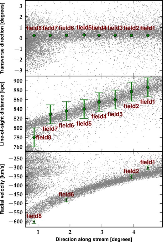
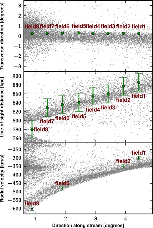
Next, we make a more in depth analysis of the spherical (Plummer) and the disc6 models by testing them against distance and kinematic data. Fig. 4 shows the distribution of satellite particles (grey dots) for the Plummer model together with the eight fields of the position and velocity observed data (McConnachie et al. 2003; Ibata et al. 2004; Gilbert et al. 2009). The upper panel corresponds to the projection in a sky coordinate system rotated such that the x-axis is aligned with the stream and the y-axis increases in the direction orthogonal to the stream. In this projection, the centre of M31 is still located at the origin. We confirm that the morphology and spatial extent of the simulated stream agrees well with the position of the observed fields.
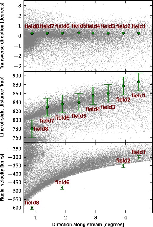
Comparison of N-body results from the Plummer model with positional and kinematical data of the GSS: position in stream-aligned coordinates (top panel), heliocentric distance (middle panel) and radial velocity (bottom panel) as a function of distance along the stream. Green filled circles show the data points corresponding to the fields 1–8 of McConnachie et al. (2003). Radial velocity measurements are taken from Ibata et al. (2004) and are only available in four of these fields. The particles of the progenitor in our simulation are represented as grey dots. The model is able to fit reasonably well the observations and can reproduce the distance–position correlation quite well. However, the phase plot (bottom panel) shows clearly that the velocity along the stream is mostly underestimated.
The middle and bottom panels show, respectively, the heliocentric distance and radial velocities as a function of distance along the stream. The observed line-of-sight distances are reproduced remarkably well by the N-body model which not only matches the observed values in individual fields but also the gradients along the axis of the stream. The only exception is for field 8 which is the nearest field from the centre of M31. Therefore, it is likely that the distance estimate in this field is contaminated by M31 stars. The radial velocities, on the other hand, show larger discrepancy especially near the M31 disc. Apart from the first observational data farthest from M31, velocities along the stream are systematically underestimated.
Fig. 5 shows the distribution of satellite particles in model Disc6 at T = 840 Myr where the different panels refer to the same quantities as their correspondences in Fig. 4. The overall distribution of stream particles agrees with the position of the observed field. However, the line-of-sight distances are underestimated as compared to the observed values. This is to be compared to the spherical Plummer model, Fig. 4, which produced a better fit to these data. The Disc model, as the Plummer model, systematically underestimates the radial velocity along the stream, as shown in the bottom panel of Fig. 5.
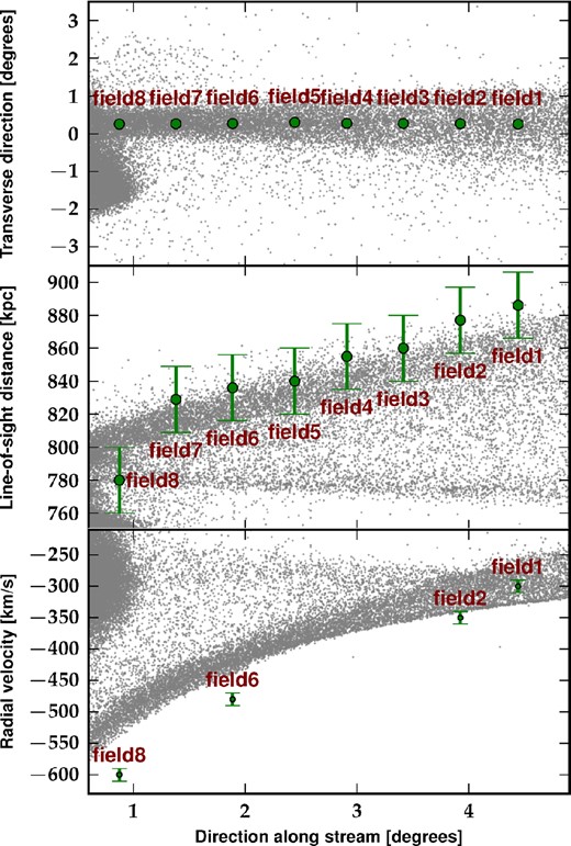
The figure compares the results from our N-body simulation for model Disc6 with the observational data. This figure is similar to Fig. 4 but is now made for a discy satellite. Compared to the spherical Plummer satellite (Fig. 4), the disc model shows a larger spread in the distance–position correlation (middle panel). A disc satellite also fails to properly model the radial velocity data which, apart from the farthest data point, are systematically underestimated (bottom panel).
Overall, we find that, to first order, there are no clear evidence to favour the disc model over the spherical Plummer model when including a live realization of M31. Both satellite morphologies are able to reproduce well the first-order properties of the stream.
3.5 Number density profiles
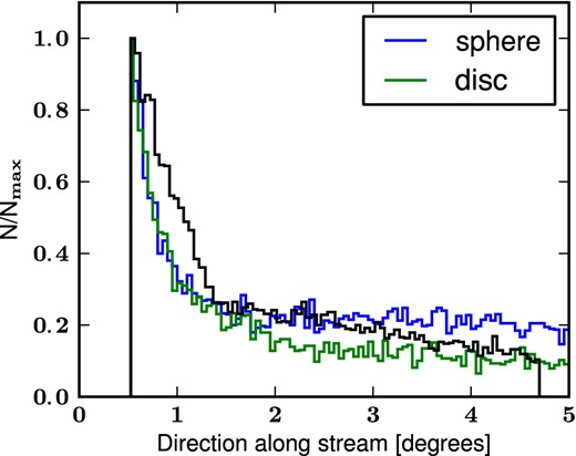
Next, we test the disc and spherical models against second-order properties of the GSS. Figs 6 and 7 show the number density profile as a function of distance parallel and orthogonal to the stream, respectively.
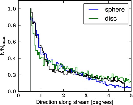
Stellar number density profile in the direction parallel to the stream. The black line shows the data from McConnachie et al. (2003). The blue line is the result from the spherical Plummer model while the green line corresponds to model Disc6. Since the number of stellar particles in the stream in our simulations is vastly superior to the number of observed stars, we normalize each profile by their respective maxima in order to be able to compare them directly to the observed profile. Furthermore, we exclude particles that are outside the region corresponding to the observed fields when calculating the profiles from our simulations.
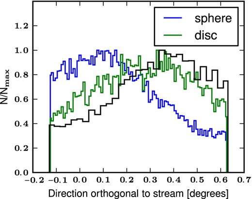
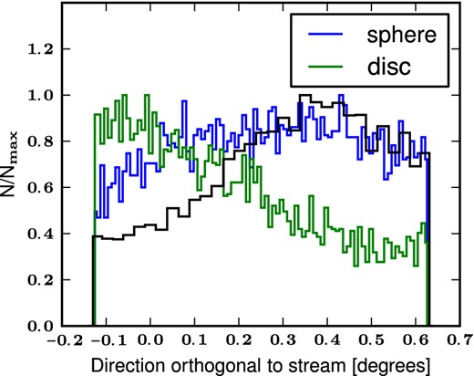
Stellar number density profile of satellite stars in the direction orthogonal to the stream. The lines have the same meaning as in Fig. 6. The GSS shows an asymmetry in the stellar distribution in the transverse direction which is better reproduced by a cold disc satellite than a dynamically hot progenitor.
Both models are able to reproduce the density profile along the stream but the spatial extension of the GSS (∼5°) is better fitted by the spherical Plummer model. Fig. 6 shows that both models produce a good approximative profile along the stream and hence these data cannot be used to prefer one over another. The observed profile in the transverse direction (Fig. 7) is asymmetric with respect to the centre of the observed fields with an excess in the NE direction. This trend is captured correctly by the disc model which uses a rotationally supported satellite (Fardal et al. 2008). On the other hand, the spherical Plummer model fails to reproduce this behaviour and, in fact, shows an excess in the south-west direction, contrary to the observational result. The orthogonal profile of the stream is the only observation clearly in favour of a discy progenitor for the empirical models whereas all other data seem to agree with both models almost equally well.
4 WHERE DID THE SATELLITE COME FROM?
So far in this work, we have used a single set of initial conditions, given by equation (5), for the progenitor satellite. This set of initial conditions assumes that the satellite started its infall on to M31 around 800 Myr ago at a separation of about 40 kpc. Although these models provide reasonable fits to the observations, they remain unmotivated and purely empirical. Satellite galaxies are not usually accreted into their host haloes for the first time from a close random distance and a satellite at a short distance from its host halo, on a highly radial orbit, is expected to have already been fully disrupted by the host on the previous pericentre passages.
If a satellite was at the origin of the GSS, then its origin itself need be properly traced back in time before a plausible set of initial conditions could be put forward. Although most galaxies host satellites, the history of these satellites and their orbital characteristics remain obscure. Within the standard model of Λ cold dark matter (ΛCDM), a hierarchical formation of galaxies favours the early formation of satellites and a later formation of their host galaxies. The initial motion of a satellite in its host potential is determined by the balance of two ‘forces’: the Hubble expansion that pushes the satellite outwards and the gravitational potential of the host halo that pulls the satellite inwards. The satellite, initially on Hubble flow, slows down under the attraction of its host galaxy until its velocity is reduced to zero at which point it separates from the background Hubble expansion, turns around and is accreted into the host galaxy. It is rather unlikely, that the satellite went through a turnaround and then arrived at the position defined by equation (5), as the present turnaround radius is by far larger than 40 kpc. [The present turnaround radius of M31 is about 1 Mpc and the turnaround radius would roughly grow as t8/9, given by a simple self-similar model (Fillmore & Goldreich 1984; Bertschinger 1985).] Satellites at such close separations from their host galaxies are most likely to have gone through a few orbits and to have arrived close to their host by losing energy through DF. However, a satellite that moves on a highly radial orbit would suffer disruption at its pericentre passages, such that it would not survive to reach a distance of 40 kpc from M31.
To study this problem in detail, we follow the trajectory of a particle in the potential of M31 back in time. Once again as for a live M31 in Section 2.1, we model M31 as a Hernquist bulge with an NFW halo, but consider a Miyamoto–Nagai potential (Miyamoto & Nagai 1975) for the disc in order to have an analytic expression for the potential. In the backward integration, we also include a ‘backward’ DF which is modelled using the well-known Chandrasekhar's formula (Chandrasekhar 1943; Binney & Tremaine 1987). Clearly, we make the simplifying assumption that the satellite loses little mass. The orbit integration is performed using a leapfrog integrator, because it is time reversible and we can explore both forward and backward orbit integrations. We begin our orbit integration from the initial condition defined by equation (5) and integrate both forwards and backwards from this point for up to t = 2 Gyr in either directions. For the backward integrations, we have considered both cases with and without the DF.
The resulting orbits are plotted in Fig. 8 which shows, in the top panel, the trajectory of the satellite in the (x, y) plane, and in the bottom panel, the evolution of its orbital radius as a function of time. The plots clearly show that DF causes the test particle to gain energy when the orbit is integrated backwards. It is also clearly seen that the satellite has had several close pericentric passages (r ∼ 1 kpc) prior to the GSS formation event. This is not entirely surprising since the characteristic of GSS constrains the satellite to be on a highly eccentric orbit. However, a dwarf galaxy such as the satellite considered here is likely to be strongly disrupted after even a single one of these close encounters with M31.
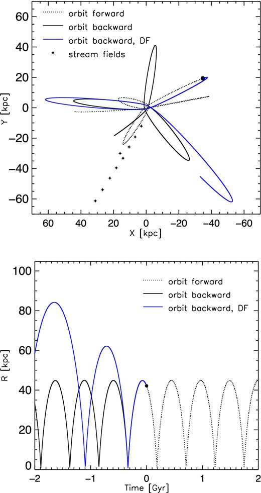
Tracing the progenitor orbit back in time: (x, y) projection (top) and orbital radius evolution (bottom) for the numerically integrated orbits for initial conditions given by equation (5) for the empirical models. The dotted line represents the forward integration from the initial point (denoted with a filled circle) while the solid lines correspond to the past of the progenitor with (blue line) and without (black line) DF.
A possible way out of this impasse would be to argue that the satellite was a compact dwarf galaxy whose core survived repeated tidal shocks when passing through M31 (Ibata et al. 2004). As a consequence, M32, a very dense satellite of M31, was suggested as a probable origin for GSS. However, it was noted that the velocity and internal dispersion of M31 are difficult to match with the observed kinematics of the GSS and furthermore M32 seems rather quiet and unperturbed. It is worth mentioning that a collision between M32 and M31 has been investigated numerically in order to explain the ring structures observed at infrared wavelengths in the M31 disc (Block et al. 2006). Our various test simulations have shown that even the core of a satellite would not survive too many pericentre passages. This scenario would indeed require an unrealistically overdense galaxy to survive these passages and satisfy the observed properties of the giant stream.
A different and somehow far-fetched argument in favour of such a model is to assume that the satellite actually formed at a distance of around 40 kpc from M31 a few hundreds of megayears ago. However, this is rather unlikely in a ΛCDM hierarchical model in which satellite galaxies are in general older and form earlier than their parent galaxies.
In the next section, we propose a new set of initial conditions that are cosmologically motivated and overcome the difficulties encountered in the empirical models for the formation of GSS and show that indeed such reasonably conceived models do satisfy a full range of observational constraints.
5 A DARK-MATTER-RICH SATELLITE ON ITS FIRST INFALL
5.1 Orbital parameters
In a general cosmological set up, the accretion of a satellite, initially on Hubble flow, into a galaxy occurs when it decelerates under the gravitational attraction of its host, reaches a zero velocity surface, turns around and falls back into the host potential. As the parameter space for our problem is unmanageably large, we focus the initial conditions for our simulations around these cosmologically most plausible configurations. In our model, the satellite starts its infall on to M31 from its first turnaround radius.
An estimate of the turnaround radius of the satellite can be made as follows. The turnaround radius grows, roughly, as rta ∼ t8/9 , which is given by a simple secondary infall model (Fillmore & Goldreich 1984; Bertschinger 1985) for a highly radial and smooth accretion. It has been shown that the secondary infall model represents quite well the numerical simulations in which dark matter haloes grow by clumpy accretion of satellites (Ascasibar, Hoffman & Gottlöber 2007). It is hard to estimate the present turnaround radius of M31, as Milky Way and M31 are thought to have a common halo. However, most observations put the present turnaround radius of M31 at around 1 Mpc. Hence using the above expression, we see that a few Gyr ago, the turnaround radius of M31 was ∼800 kpc.
However, since this estimate of the turnaround radius is associated with large uncertainties (partly because, as we said, it is hard to disentangle the contribution from Milky Way and M31 haloes), we consider the following argument. To further constrain the initial radius of the accreted satellite, we can use the current extent of the stream as a rough indicator of the initial distance from which the satellite fell into M31 potential. This assumption is reasonable because, in our model, the satellite falls for the first time towards M31 on a nearly radial orbit and the stream is produced from tidal debris after the first close encounter. Therefore, the extent of the stream should roughly be of the same order as the apocentre of the initial orbit of the satellite. Based on these considerations, we estimate the initial infalling radius of the satellite to be ∼ 150-200 kpc. We run around 40 full N-body simulations to fine-tune in this part of the parameter space.
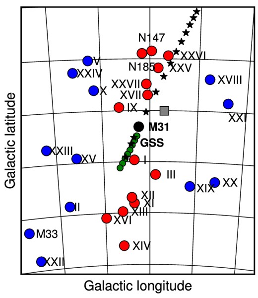
The sky map of the satellites of M31 is shown (see Conn et al. 2013; Ibata et al. 2013 for full details). We have shown the positions of the giant stream (GSS) by the filled green circles. The grey box shows the initial position for the GSS progenitor in the previous empirical models (see equation 5 in Section 3). The orbit of the progenitor satellite given by the N-body simulation of our first-infall model (see Section 5) is shown by stars, which lies almost on the same thin plane as most of the satellites of M31. In our model, the progenitor satellite is accreted from a large first turnaround distance of about 200 kpc.
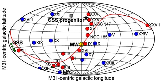
This map is similar to Fig. 9 but all positions are now viewed from Andromeda. We show the initial position of the satellite in our first-infall model (see equation 6 in Section 5) by star. The thin plane containing many of the M31 satellites is also drawn (see Conn et al. 2013; Ibata et al. 2013 for full details). The position of the giant stream (GSS) is also shown on this map by green filled circles.
A satellite on such an orbit would have a very large velocity at the pericentre passage and would not be able to account for the large mass of the GSS, as it would lose too little mass. However, it could slow down by DF, which can be significant if the satellite is dark matter rich. Therefore, we consider a dark-matter-dominated satellite which is also consistent with the observation of most Local Group dwarfs (see e.g. Mateo 1998). We assume that the stellar mass of the satellite is still the same as we used for the empirical models, i.e. Ms = 2.2 × 10⁹ M⊙, studied in Section 3. This assumption is reasonable as the stellar mass of the satellite is relatively well constrained by the stellar mass of the GSS (Fardal et al. 2006). In our best-fitting initial conditions, the ratio of total to stellar mass is M/Ms = 20 and the halo has a mass of MDM = 4.18 × 10¹⁰ M⊙. Interestingly, this implies that the satellite lies below the stellar to halo mass relation as galaxies in this mass range have a mean halo mass of ∼2 × 10¹¹ M⊙ (Behroozi, Wechsler & Conroy 2013).
In our simulations, the dark halo is represented as a spherical Hernquist profile with a scale radius of rh = 12.5 kpc sampled with Nh = 124 405 particles, yielding a mass resolution of mh = 3.36 × 10⁵M⊙ for dark matter particles. The satellite starts initially at r ∼ 200 kpc and is followed up to r ∼ 40 kpc. Concerning the morphology of the satellite, we use the same sets of models that were described in Section 2.2 supplemented with an additional component representing the dark matter halo. The N-body realizations of the models are carried out with nbodygen for the spherical profiles and with the Gaussian approximation method detailed in Section 2.1 for the disc profiles.
5.2 Spatial extent, morphology and stellar mass
In order to assess the ability of our model to reproduce the GSS observations, we perform a similar analysis as we did in Section 3. As before, the total time T of the simulation is chosen such that to obtain a best match between our simulated stream and the GSS. With our cosmologically motivated scenario, we find T = 2.7 Gyr. Thus, the overall merger time-scale in our scenario is much longer than for the empirical models which had T = 0.84 Gyr.
This longer time-scale also implies that, in our model, the satellite had not experienced recent star formation when it started its infall in M31 halo since the minimum stellar ages in the Giant stream have been estimated to be at least 4 Gyr (Brown et al. 2006). This is potentially in contradiction with recent studies showing that most dwarf galaxies need to be near a massive host in order to quench their star formation (Geha et al. 2012). However, the satellite is slightly more massive than the typical dwarfs considered in these studies and could have been located within a few virial radius from M31 halo before its infall which is the region where Geha et al. (2012) find quenched galaxies. Furthermore, it is possible that the satellite had a peculiar star formation history, compared to the majority of dwarfs, since it also seems to have a peculiar orbital history in order to be on such eccentric orbit.
First, we test the spatial distribution, morphology and stellar mass in the stream. Fig. 11 shows the real space (left-hand panel) and phase-space (right-hand panel) projections of stellar particles initially in the satellite similarly to Fig. 1. For clarity, the dark matter particles of both M31 and the satellite have been omitted from these plots. We trace the orbit of the satellite by following the initially most bound particles in our simulation. The resulting trajectory is represented as a dashed line in the real space projection and shows that the merger is almost a head-on collision between M31 and the satellite. We are also able to identify the tidal structures in phase space and find again the presence of an extended stream and two caustics formed by coherent group of particles with same number of pericentric passages.
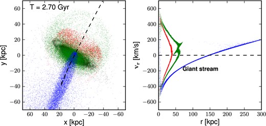
Distribution of stellar particles in the satellite in the x-y plane (left-hand panel) and the phase plot in the r-vr plane (right-hand panel) at t = 2.7 Gyr for our first-infall N-body model using a spherical progenitor. The plots represent the same quantities as in Fig. 1 but are now made for our first-infall model. Although difficult to identify in real space, the presence of two tidal caustics corresponding to a second and a third orbital wrap are clearly seen in the phase space (right-hand panel). The NE shelf shown in green and the W shelf shown in red, near the zero velocity surfaces, correspond to stars on their second and third pericentre passages, respectively. The position of the remnant of the satellite, which lies in the region of the NE shelf, is clearly seen in this plot which is in agreement with results from a recent statistical approach (Fardal et al. 2013).
The stellar density maps in sky coordinates compared to the position of the observed fields of the GSS and the edges of the two shelves are shown in Fig. 12. We obtain a good agreement between the spatial distribution and morphology of our simulated stream and the GSS in the case of the spherical Plummer model. However, the phase-space projection (right-hand panel of Fig. 12) indicates that the edges of the shelves are located further than 50 kpc and thus overestimated by the model when compared to the observed value. We also find that the simulated stream extends beyond the current length estimates although the distance of ∼150 kpc at which stream stars turn back (vr = 0 in the right-hand panel of Fig. 11) matches the observed stream apocentre of ∼140 kpc (Ibata et al. 2007). The part of the simulated stream extending beyond this point might be too diluted, due to the large stretching of tidal debris in our model, to be able to be detected by current surveys. On the other hand, the disc model is unable to reproduce correctly the angular direction of the stream. We also calculate the stellar mass of the simulated stream and find MGSS = 1.912 × 10⁸ M⊙ for the spherical model in good agreement with the estimated GSS mass and MGSS = 1.121 × 10⁸ M⊙ for the disc model as indicated by Fig. 12. This further confirms that the disc model provides a poorer fit to the GSS than a spherical satellite.
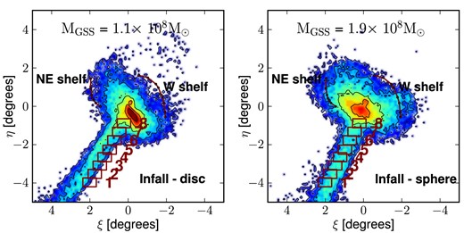
Stellar density maps in standard sky coordinates similar to Fig. 2 but for our cosmologically motivated ‘first-infall’ model plotted for a cold discy progenitor (left-hand panel) and a hot spheroidal dwarf progenitor (right-hand panel). Our simulations favour a dynamically hot spheroidal dwarf over a cold discy progenitor.
5.3 Distance and kinematics
Next, we examine the three-dimensional distribution of the stream and its kinematics. Figs 13 and 14 show the comparison between our simulated stream and observations, similar to what we did in Figs 4 and 5 for empirical models. We obtain an excellent agreement with observations for both the spatial distribution as well as the heliocentric distance and radial velocity measurements. The agreement is significantly better for the spherical model than for the disc model. In particular, for the spherical model, the scatter in the distance–position correlation is fully consistent with the distance error estimates from McConnachie et al. (2003) except for field 8 which is most-likely due to contamination from M31 disc stars since this field is the closest from M31 centre.
Comparison of results from our N-body simulation of the first-infall model using a spherical Plummer satellite with observational data for the GSS. The figure is similar to Fig. 4. Our cosmologically motivated first-infall scenario for the formation of the giant stream successfully reproduces the stream's three-dimensional position and kinematics.
Comparison of results from our N-body simulation of the first-infall model using a discy satellite (grey dots) to the observational data (green points with error bars). The figure is similar to Fig. 4. The agreement with the data is poorer than that of our model with a spherical progenitor (see Fig. 13).
The kinematic data, from the observations of GSS, provide a strong evidence in support of our model. The phase plot, bottom panel in Fig. 13 follows the motion of the satellite as it falls into and is disrupted by M31 and forms the giant stream. Our simulations show that the kinematic data favours an infall from a large initial radius. Previous empirical models produce a less satisfactory agreement with the velocity data and have a large velocity offset, because in these models, studied in Section 3, the satellite starts its infall at a short distance of about 40 kpc from M31 and hence the velocity of stream particles, throughout the orbit, are smaller than suggested by the observations. A short initial infall radius means a shorter subsequent apocentre and hence a smaller velocity along the trajectory.
5.4 Number density profiles
We also investigate the density profiles of the stream in our models. Similarly to the procedure described in Section 3, we only consider particles in the region defined by the observed fields. Fig. 15 shows the density profile in the direction parallel to the stream. We find that, for both the spherical (blue line) and the disc (green line) models, the shape of the simulated profile differs slightly from the observed one (black line). In our models, the density decreases more rapidly in the inner region of the stream but presents a shallower slope at large distances.
Density profile of satellite stars calculated in the direction parallel to the stream (same as done for Fig. 6) for our first-infall models. The black line shows the data from McConnachie et al. (2003). The blue line is the result from the spherical Plummer model while the green line corresponds to a discy satellite. We find minor deviations from the observed profile (black line) with a steeper shape at small distances and a shallower behaviour at large radii for both a spherical (blue line) or disc (green line) satellite. The length of the stream is broadly consistent with its observed value.
The density profile in the transverse direction is shown in Fig. 16. For our first-infall scenario, the spherical model reproduces well the asymmetric profile orthogonal to the stream but the disc model fails to do so. However, since the disc model produces a stream that is offset from the observed fields (see left-hand panel of Fig. 12), the density profile transverse to the direction defined by the observed stream is expected to be underestimated as we find here.
Density profile of satellite stars calculated in the direction transverse to the stream as presented previously in Fig. 7 but now for our first-infall models. The black line shows the data from McConnachie et al. (2003). The blue line is the result from the spherical Plummer model while the green line corresponds to a discy satellite. The spherical progenitor clearly reproduces better the asymmetric shape of the profile than the discy satellite.
5.5 Velocity dispersion
So far, we have compared the kinematics of the stream with the observed GSS kinematics using the radial velocity measurements given by Ibata et al. (2004). However, we can further test the viability of our model by comparing the velocity dispersion at difference radii from the centre of M31, to those given by the observations. From the radial velocity measurements in fields 1, 2, 6 and 8 (Ibata et al. 2004), the mean observed velocity profile along the stream has been found and fitted by vh(η) = −4244.8tan η − 610.9 kms, where η is the north–south direction in standard sky coordinates. It is then possible to derive an estimate of the velocity dispersion along the stream as the offset between this mean profile and the velocity of each stellar particle.
We show in Fig. 17 the distribution of velocity offsets calculated for both the empirical modelling of the orbit with Rinit = 40 kpc (first row), discussed in Section 3 and for our first-infall models with Rinit = 200 kpc (bottom row). In each row, the left- and right-hand panels correspond, respectively, to the result obtained using a spherical and a disc satellite. In each panel, the green histogram is the result calculated from stellar particles in our simulated stream and the black histogram is the distribution from the observations (Ibata et al. 2004). We fit a Gaussian distribution to the histogram to estimate the dispersion in the stream, similar to the procedure used by Ibata et al. (2004). They estimate the velocity dispersion in the stream to be σ = 11 ± 3 kms. We find that all models tend to overestimate the dispersion in the stream. However, the best match between the observed and estimated distributions is obtained for our cosmologically motivated first-infall scenario with a spherical Plummer satellite. The small apocentre of the satellite trajectory in the empirical models, studied in Section 3, is the reason for the systematic underestimation of the velocities.
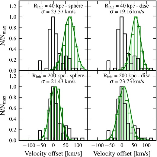
Velocity distribution of stream particles in four different N-body simulations of the models that successfully reproduce the positional data as well as the distance and velocity gradients along the stream. The black histogram is given by the observations (Ibata et al. 2004) and the green by our four simulations. The smooth green curves are the Gaussian fits. The models with a dark-matter-poor satellite that use the initial phase coordinates of equation (5) are in the top panels whereas our first-infall models, which use a dark-matter-rich satellite with the initial orbital parameters given by the equation (6), are shown in the bottom panels. The left-hand column shows the case of a spherical satellite and the right-hand column the case of a disc satellite. All the models are roughly consistent with the velocity dispersion derived from the observed GSS kinematics (Ibata et al. 2004). The cosmologically motivated first-infall model (lower panels) has the least offset w.r.t. the observations.
5.6 Dark-matter-poor versus dark-matter-rich progenitor satellite
Our best-fitting model favours a dark-matter-rich spheroidal dwarf galaxy as the progenitor of the GSS. However, one might argue that dark matter halo would play a marginal role in the formation of the GSS, as most of it is stripped off the satellite long before it passes through M31. In this section, we shall use our N-body simulations to study this question.
We quantify the mass-loss experienced by the satellite in our first-infall model.
To obtain an estimate of the mass-loss from the satellite, we compute the dark matter mass Mi(<ri) that encloses a fixed radius ri as a function of time. The evolution for ri = 1, 2, 5, 10, 20 and 50 kpc is plotted in Fig. 18. The pericentre occurs for t/t0 ∼ 0.85 where t0 is defined as the time at which the satellite reaches r ∼ 40 kpc which is the starting point for the empirical models, discussed in Section 3. The halo is largely unaffected up to t/t0 ∼ 0.6 at which point it starts to significantly deform due to the M31 tidal field. Nevertheless, the satellite is able to retain a large portion of its mass up to t = t0 where it has already reached a distance of 40 kpc from M31. In the end, the dark matter halo can still contribute to a large fraction of the satellite mass up to the formation of GSS. The orbital history of the satellite, reconstructed from simulations using either no or only simple analytical treatment of DF might give contradictory results. However, we argue that full N-body simulations, which incorporate the central galaxy as an N-body system as we have done here, are necessary to fully model the mass-loss for the unusual cases of highly eccentric orbits.
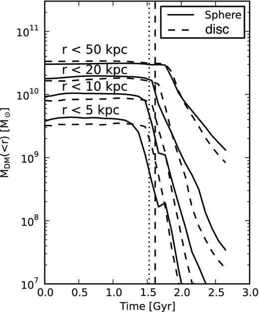
Evolution of the enclosed dark matter mass MDM(<r) of the satellite as a function of time for different radii r in our first-infall N-body models. The solid and dashed line correspond to a spherical or a disc progenitor, respectively. The vertical dotted line indicates the time when the satellite is at r ∼ 40 kpc, which is the starting point for various empirical models, discussed in Section 3. The vertical dashed line corresponds to the pericentric passage. Due to the highly eccentric orbit required to reproduce the GSS, in both models the satellite is able to retain a significant fraction of its dark matter halo as it falls towards M31 from 200 to 40 kpc.
6 THE WARP OF M31 DISC
The presence of a warp in the neutral hydrogen disc of M31 has been known for some times (Baade & Swope 1963; Roberts 1966; Newton & Emerson 1977; Whitehurst, Roberts & Cram 1978; Innanen et al. 1982; Ferguson et al. 2002; Richardson et al. 2008). Indeed, warps seem to be a common feature of many galaxies and it has been shown that of the order of half of all galactic H i discs are measurably warped, as is the disc of the Milky Way (Bosma 1978). Briggs (1990) studied the warps of a sample of 12 galaxies in detail and inferred several general laws that govern the phenomenology of warps. In the years that followed Briggs’ work, many more catalogues of warp galaxies have been developed (see e.g. Reshetnikov & Combes 1999; Sánchez-Saavedra et al. 2003). The fact that stellar warps usually follow the same warped surface as do the gaseous ones (e.g. Cox et al. 1996) is a strong evidence that warps are principally a gravitational phenomenon.
The origin of warps remains unclear but numerous theories based on the interaction between the disc and the halo, or the cosmic infall and tidal effects, or non-linear back-reaction from the spiral arms, or modified gravity have been proposed (e.g. see Ostriker & Binney 1989; Binney 1992; Quinn & Binney 1992; Nelson & Tremaine 1995; Masset & Tagger 1997; Jiang & Binney 1999; Brada & Milgrom 2000; López-Corredoira, Betancort-Rijo & Beckman 2002; Sánchez-Salcedo 2006; Shen & Sellwood 2006; Weinberg & Blitz 2006).
In this work, we study the formation of the warp of M31 as a result of the infall of the satellite progenitor of the giant stream. Up to now, we have only studied the tidal effect of M31 on the infalling satellite. However, as our satellite is massive, the disc of M31 could also become heated and perturbed during this infall. A few snapshots of the evolution of the disc of M31 is shown from the beginning of the simulation to the end in Fig. 19. The figure clearly shows that the disc becomes tilted, heated and warped as the infalling satellite approaches and goes through M31.
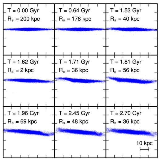
Edge-on view of the M31 disc at different times in our first-infall model with a spherical infalling satellite. The disc is visibly perturbed by the passage of the satellite and exhibits a warp-like structure at later times. The time after the start of the simulation and the orbital radius Rs, which is the distance of the centre of mass of the satellite to M31, is indicated in each frame.
To study these effects quantitatively, we first calculate the vertical height profile of the disc, 〈z2〉1/2, as a function of the cylindrical radius R by dividing the disc in concentric rings and computing their root mean square elevation above the z = 0 plane defined to be the plane of the disc before the passage of the satellite. We also compute the vertical velocity dispersion, |$\left\langle \sigma _z^2\right\rangle ^{1/2}$|, in each ring. For comparison, we also calculate the same quantities for the empirical models of GSS formation which rely on a dark-matter-poor satellite (discussed in Section 3). We find that, in our first-infall model, after the passage of the GSS progenitor, the disc thickness increases, as shown in Fig. 20, and the scaleheight reaches about 2 kpc, in good agreement with the observations that give an average scaleheight of 2.8 ± 0.6 kpc for the thick disc of M31 (Collins et al. 2011). Although the satellite is dark matter rich and massive, its rapid passage through M31 guarantees that the disc of M31 is not destroyed or heated to extreme. It has previously been suggested that minor mergers could be at the origin of the thick discs of galaxies (Purcell, Bullock & Kazantzidis 2010) and in our work we clearly see that the infall of the progenitor of the GSS could be partially responsible for the thick disc of M31.
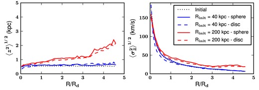
Heating of the disc of M31 due to the perturbations from the satellite in the N-body models that we studied in this work. The results are shown for both discy and spherical progenitors and also for empirical models with a dark-matter-poor satellite (Rinit = 40 kpc), studied in Section 3, and our first-infall models with a dark-matter-rich satellite (Rinit = 200 kpc), studied in Section 5. Mean vertical height 〈z2〉1/2 and the vertical velocity dispersion |$\left\langle \sigma _z^2\right\rangle ^{1/2}$| as functions of cylindrical radius in units of the scale radius Rd = 5.4 kpc (see Table 1) of the disc are plotted. In both of our first-infall models, the passage of the satellite significantly disturbs the disc because the progenitor retains a large fraction of its dark matter mass. The panels show that the outer regions of the disc (R > 2Rd) are heated and become thicker with respect to the inner parts, in our cosmologically motivated first-infall model.
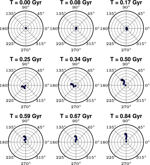
The passage of the satellite through M31 also causes the disc of the galaxy to warp. In general, the integral-sign warps can be viewed as the m = 1 or s-wave perturbations that are excited in the disc by various sources (Hunter & Toomre 1969) and in our case by the passage of the satellite. Warps are characterized by their lines of nodes and inclination angles (Briggs 1990). The diagram of the line of nodes is an unusual polar plot of the angle made by the line of nodes and the latitude of the concentric rings into which the disc of the galaxy is divided, for the purpose of the study of the warps. The line of nodes for our model develops into a spiral, as shown in Fig. 21, due to the differential rotation of the disc, with a twist and a winding period of about 3 Gyr which are all generic characteristics of galactic warps (Briggs 1990; Shen & Sellwood 2006). The observations find that the extended disc of M31 is about 30 kpc and its H i warp starts at around 16 kpc (Newton & Emerson 1977; Henderson 1979; Brinks & Burton 1984; Chemin, Carignan & Foster 2009) and the scaleheight of the gas layer reaches a maximum value of about 2 kpc. These values agree reasonably with our results, although we find that the scaleheight starts increasing at smaller radii for a stellar warp.
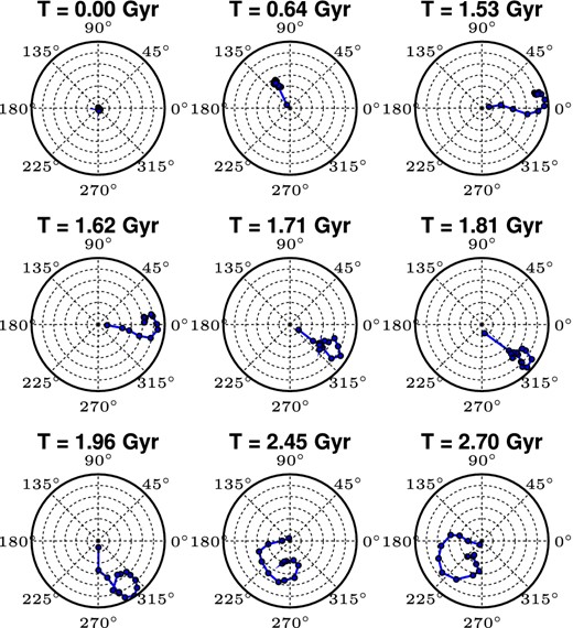
The diagram of the line of nodes showing the time evolution of the warp of M31 in our first-infall model, discussed in Section 5. The snapshots are shown from the start of the simulation (T = 0 Gyr) to the last time step (T = 2.7 Gyr) which corresponds to the present time. To make this diagram, the disc of M31 is divided into concentric annuli of width of about 1 kpc starting at 3 kpc from the centre of M31 disc. The radial coordinate is the warp or inclination angle that an annulus of the disc makes with the inner disc plane, shown at 1° intervals. The azimuthal coordinate gives the azimuth of the line of nodes. The solid points are plotted for the radially ordered annuli at 1 kpc intervals, apart from the first central point which is averaged over 3 kpc annulus. At the start of our simulation, there is no warp, and all points crowd at the centre of the diagram. After the passage of the satellite through M31, the line of nodes first form a straight line and then form a spiral when the differential rotation sets in (Briggs 1990). The warp rotates clockwise and has a winding period of about 3 Gyr.
To demonstrate that the warps are indeed due to the passage of our massive satellite, we also make a similar plot of the line of nodes, in Fig. 22, for the empirical model that we studied in Section 3. Although perturbed and slightly heated, the disc is not warped in these models, which is expected since the satellite is dark matter poor and starts its journey from a short distance of 40 kpc from M31.
The figure is the same as Fig. 21 but here is made for the empirical models (see Section 3), with a spherical Plummer satellite. The snapshots are shown for this model from the start of the simulation (T = 0 Gyr) to the last time step (T = 0.84 Gyr) which corresponds to the present time. The satellite is dark matter poor and falls from a short distance of 40 kpc on to M31 and, as expected, only weakly perturbs the disc but cannot cause it to warp.
7 CONCLUSION
A wide range of observational data has progressively become available for the Andromeda galaxy. The disc of Andromeda is not flat but is distorted and warped. Its outskirts also seem drastically perturbed and a giant stellar stream, extending over tens of kiloparsecs, flows directly on to the centre of Andromeda. The galaxy has about 30 satellites, observed so far, many of which seem to be corotating on a thin plane. These features have often been studied as unrelated events. Here we have aimed at providing a unique scenario that would fit these puzzling aspects of M31. We have shown that the accretion of a dark-matter-rich dwarf spheroidal provides a common origin for the GSS and the warp of M31, and a hint for the origin of the thin plane of its satellites.
In our cosmologically motivated model the trajectory of the progenitor satellite lies on the same thin plane that presently contains many of M31 satellites and separates from the Hubble expansion at about 3 Gyr ago and is accreted from its turnaround radius, of about 200 kpc, into M31. It is disrupted as it orbits in the potential well of the galaxy and consequently forms the giant stream and in return heats and warps the disc of M31. The position of the GSS and the two shelves is reproduced by our full N-body simulations which use a live M31. The observed mass of the GSS obtained from its luminosity, is also predicted by our model, which is in particular favoured by the kinematic data. A prediction of our model is the actual position of the remnant of the progenitor satellite which should be found behind the NE shelf.
As the satellite is dark matter rich its infall perturbs the disc of M31. The thickness of the disc of M31 increases by a few kpc and we have also shown that the lines of node clearly indicate the presence of a warp with an angle going to about |$6^{^\circ }$|, which agrees with the observations.
The stringent constraints set by a full range of observations on the initial conditions strongly suggest that the satellites of M31, which presently corotate on the same thin plane as our progenitor dwarf, could have similarly been accreted on to M31 along an intergalactic filament, which is yet to be identified by the observations. The orbit of the progenitor satellite lies very close to the direction of M31–M33, as shown in Figs 9 and 10, which could be along an intergalactic filament (Wolfe et al. 2013), yet to be confirmed by observations. Although not included, it is plausible that the gas which could have been contained within our massive satellite would also be disrupted during its passage through M31 and could contribute to the puzzling H i filament that joins M31 and M33 (Wolfe et al. 2013) which also has been found to correlate, at least partially, with the GSS of M31 (Lewis et al. 2013).
We thank Wyn Evans, Francois Hammer, Rodrigo Ibata, Youjun Lu, Jim Peebles, Robyn Sanderson, Scott Tremaine and Qingjuan Yu for discussions.
Available publicly at http://www2.iap.fr/users/sadoun
