


Abstract
We present diffuse Lyα haloes (LAHs) identified in the composite Subaru narrow-band images of 100–3600 Lyα emitters (LAEs) at z = 2.2, 3.1, 3.7, 5.7, and 6.6. First, we carefully examine potential artefacts mimicking LAHs that include a large-scale point-spread function made by instrumental and atmospheric effects. Based on our critical test with composite images of non-LAE samples whose narrow-band-magnitude and source-size distributions are the same as our LAE samples, we confirm that no artefacts can produce a diffuse extended feature similar to our LAHs. After this test, we measure the scalelengths of exponential profile for the LAHs estimated from our z = 2.2–6.6 LAE samples of LLyα ≳ 2 × 1042 erg s−1. We obtain the scalelengths of ≃5–10 kpc at z = 2.2–5.7, and find no evolution of scalelengths in this redshift range beyond our measurement uncertainties. Combining this result and the previously known UV-continuum size evolution, we infer that the ratio of LAH to UV-continuum sizes is nearly constant at z = 2.2–5.7. The scalelength of our z = 6.6 LAH is larger than 5-10 kpc just beyond the error bar, which is a hint that the scalelengths of LAHs would increase from z = 5.7 to 6.6. If this increase is confirmed by future large surveys with significant improvements of statistical and systematical errors, this scalelength change at z ≳ 6 would be a signature of increasing fraction of neutral hydrogen scattering Lyα photons, due to cosmic reionization.
1 INTRODUCTION
The circumgalactic medium (CGM) is closely related to galaxy formation and evolution. Gas inflows into galaxies could trigger starbursts (e.g. Dekel et al. 2009a; Dekel, Sari & Ceverino 2009b), while gaseous outflows are thought to be a physical process of quenching star formation (e.g. Mori, Ferrara & Madau 2002; Scannapieco, Silk & Bouwens 2005; Mori & Umemura 2006; Davé, Oppenheimer & Finlator 2011). The distribution of the CGM is characterized by Lyα emission, because Lyα photons escaping from a galaxy are resonantly scattered by surrounding neutral hydrogen gas. The scattered light would produce diffuse Lyα emission around a galaxy. This spatially extended Lyα emission is dubbed Lyα halo (LAH). Numerical simulations have predicted that LAHs are ubiquitously present around high-z galaxies (e.g. Laursen & Sommer-Larsen 2007; Zheng et al. 2011; Dijkstra & Kramer 2012; Verhamme et al. 2012).
Radial surface brightness (SB) profiles of the LAHs are useful to understand kinematic properties of CGM and neutral hydrogen fraction of intergalactic medium (IGM) at the epoch of cosmic reionization. Zheng et al. (2011) have predicted that the slope of a radial SB profile depends on an outflowing velocity of CGM based on their radiative transfer model. Dijkstra & Kramer (2012) have calculated radiative transfer of Lyα photons propagating through clumpy and dusty large-scale outflowing interstellar medium (ISM), and reproduced an extended Lyα structure. Furthermore, Jeeson-Daniel et al. (2012) demonstrate that radial SB profiles of LAHs are flatter at the epoch of reionization than at the post-reionization epoch, due to Lyα photons scattered by neutral hydrogen of IGM. On the other hand, recent observations find no diffuse metal-line emission of hot ionized gas around high-z galaxies on average (Yuma et al. 2013), and indicate that LAHs are probably not made by emission of hot CGM given by outflow, but by the other physical processes of cold CGM.
Extended Lyα emission has been observed around nearby star-forming galaxies (e.g. Östlin et al. 2009; Hayes et al. 2013, 2014) and QSOs (e.g. Rauch et al. 2008; Goto et al. 2009). However, LAHs are too diffuse and faint to be detected for high-z galaxies on an individual basis. LAHs at z ≥ 2 are found in stacked data of ∼20–2000 narrow-band (NB) images of high-z galaxies in previous studies. Hayashino et al. (2004) have discovered an LAH around Lyman break galaxies (LBGs) at z = 3.1 with their composite NB image. Steidel et al. (2011) have identified extended LAHs with a radius of r ∼ 80 kpc around LBGs at a spectroscopic redshift of 〈z〉 = 2.65 by stacking 92 NB images. Matsuda et al. (2012) have stacked 130–864 LAEs at z = 3.1, and detected LAHs. On the other hand, Jiang et al. (2013) have found no extended Lyα emission in their composite image produced with dozens of LAEs at z = 5.7 and 6.6, although their results are based on the small statistics.
There is an argument of systematic uncertainties producing spurious features similar to LAHs (Feldmeier et al. 2013). Feldmeier et al. (2013) have claimed that one of major sources of spurious LAHs is a large-scale point-spread function (PSF) that appears in deep images taken by ground-based observations (King 1971). A profile of large-scale PSF is largely extended, and the slope of profile changes at large radii of > 4 arcsec (Feldmeier et al. 2013), probably due to atmospheric turbulence and instrumental conditions (e.g. Racine 1996; Bernstein 2007). The profile of large-scale PSF can mimic that of LAH, and would be mistakenly identified as an LAH. Thus, the existence of LAHs is still under debate. In order to test the existence of LAHs, a careful data analysis as well as a large galaxy sample is required.
Here, we present our analysis and results of LAHs at z = 2.2–6.6 based on our large LAE samples given by Subaru NB observations (Ouchi et al. 2008, 2010; Nakajima et al. 2012). The large LAE samples of high-quality Subaru images enable us to test the existence of diffuse LAHs and to extend the study from z ∼ 2–3 to 6.6. We show the data and analysis in Section 2, systematic errors in Section 3, and our results of LAHs in Section 4, and discuss galaxy formation and reionization in Section 5. We summarize our results and discussions in Section 6. Throughout this paper, we use AB magnitudes and adopt a cosmology parameter set of (Ωm, |$\Omega _\Lambda$|, H0) = (0.3, 0.7, 70 km s−1 Mpc−1). In this cosmology, 1 arcsec corresponds to transverse sizes of (8.3, 7.6, 7.2, 5.9, 5.4) kpc at z = (2.2, 3.1, 3.7, 5.7, 6.6).
2 DATA AND ANALYSIS
2.1 Data set
We use large photometric samples of LAEs at z = 2.2, 3.1, 3.7, 5.7, and 6.6 made by the large-area NB imaging surveys of Subaru telescope. Our z = 2.2 sample consists of 3556 LAEs found in five deep fields of COSMOS, GOODS-N, GOODS-S, SSA22, and SXDS (Nakajima et al. 2012). The total area of the deep fields with our z = 2.2 LAEs is about 2.3 deg2. The z = 2.2 LAEs are identified by an excess of flux in an NB of NB387 whose central wavelength and full width at half-maximum (FWHM) are 3870 and 94 Å, respectively. The continua of these LAEs are determined with V-band images taken by Capak et al. (2004), Hayashino et al. (2004), Taniguchi et al. (2007), Furusawa et al. (2008), and Taylor et al. (2009). Our z = 3.1–6.6 LAE samples are obtained only in the 1 deg2 SXDS field (Ouchi et al. 2008, 2010). There are (316, 100, 397, 119) LAEs at z = (3.1, 3.7, 5.7, 6.6) identified with NBs of (NB503, NB570, NB816, NB921). The central wavelength and FWHM values are (5029, 74 Å), (5703, 69 Å), (8150, 120 Å), and (9196, 132 Å) for NB503, NB570, NB816, and NB921, respectively. The continua of LAEs are estimated with broad-band images of R, i′, z′, and J bands for NB503, NB570, NB816, and NB921 LAEs. We refer to these broad-band images for our continuum estimates as continuum images. These optical and near-infrared images are taken from the public data of SXDS (Furusawa et al. 2008) and UKIDSS (Lawrence et al. 2007), respectively. All of the imaging data used in this study are obtained with Subaru/Suprime-Cam (Miyazaki et al. 2002), except for the J-band image. The J-band observations are conducted with the Wide Field Camera (Hewett et al. 2006; Casali et al. 2007) on the UK Infrared Telescope. In summary, our samples have a total of 4488 LAEs at z = 2.2–6.6 on the 2.3 deg2 sky. Our LAE samples have the Lyα luminosity and equivalent-width limits of ∼1042 erg s−1 and ∼20–60 Å, respectively (Section 4.2; see Ouchi et al. 2008, 2010; Nakajima et al. 2012 for more details). Our LAE samples include 83, 41, 26, 17, and 16 spectroscopically confirmed LAEs at z = 2.2, 3.1, 3.7, 5.7, and 6.6, respectively (Ouchi et al. 2008, 2010; Nakajima et al. 2012, 2013; Hashimoto et al. 2013; Shibuya et al. 2014b; Nakajima et al., in preparation). These spectroscopic studies find that the contamination rate of these LAE samples is negligibly small, ∼0 per cent. The contamination rate can be up to only ∼30 per cent, even if all of the unidentified objects near the flux limits of spectroscopy are regarded as contamination sources. No redshift dependence of contamination rate is reported in these spectroscopic studies. Because our LAE samples should include some contamination sources, the effect of contamination is discussed with the results of mean and median statistics in Section 4.2.
2.2 Image stacking
To investigate LAHs, we carry out stacking analysis with the continuum and NB images of our LAEs.
Smoothing images We smooth all the continuum and NB images with Gaussian kernels to match their seeing sizes to an FWHM of 1.32 arcsec that is the largest PSF size among the images.
Subtracting continuum fluxes We subtract the smoothed continuum images from the smoothed NB images under the assumption of fν =const. The NB images with a continuum subtraction are referred to as Lyα images.
Making cutout images We make cutout images of the smoothed continuum and Lyα images with a size of 45 arcsec × 45 arcsec centred at a position of LAE. Here, we exclude LAEs that are placed at the areas within 200 pixels from the edge of imaging data to avoid systematic effects. The numbers of our LAEs that we use are listed in Table 1.
Stacking images We stack these cutout images with the imcombine task of iraf in two ways, ‘mean-combined’ and ‘median-combined’ methods. In the mean-combined method, we adopt a weighted-mean algorithm with a 1σ noise defined in each survey field. We apply 3σ clipping to remove shot noise and accidental false signals. Because our z ≥ 3.1 LAEs are found in the single field of SXDS, we simply obtain mean-combined images with no weighting for our z ≥ 3.1 LAEs. To make the median-combined image, we normalize our LAE images with the total fluxes, and perform median stacking with a weight based on a signal-to-noise ratio of survey field. Note that additional errors from the total flux measurements are included in this normalization process, and that the median-combined images have uncertainties lager than the mean-combined images.1 After stacking the images, we degrade all of the stacked images to the same pixel size of 0.3 arcsec to construct a matched pixel size data set of composite images.2 The composite images are presented in Figs 1 and 2, and the radial SB profiles of our LAEs in the Lyα images are shown in Fig. 3. In Figs 1 and 2, the sources in the Lyα images, especially for z = 6.6 LAEs, appear slightly elongated. Because we display the images with colour scales down to ∼1σ noise levels, the elongated features are probably made by noise near the outskirts of sources.
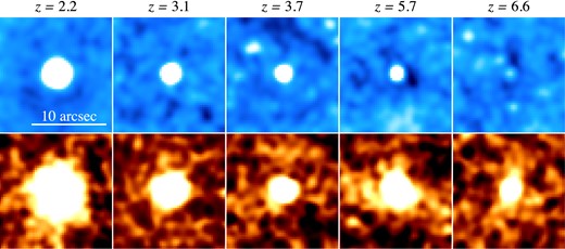
Composite continuum (top panels) and Lyα (bottom panels) images of our LAEs produced by the mean-combined method. From left to right panels, we show z = 2.2, 3.1, 3.7, 5.7, and 6.6 LAE images.
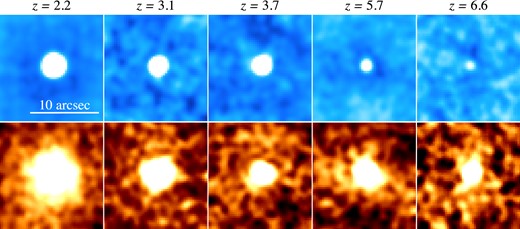
Same as Fig. 1, but for the median-combined method.

Radial SB profiles of composite images of LAEs (solid lines) and PSFs (dotted lines) at redshifts of z = 2.2–6.6. The upper and lower panels represent SB profiles of continuum and Lyα emission, respectively. The cyan and orange (blue and red) lines denote the results of mean-combined (median-combined) methods.
Samples and diffuse LAHs in our and previous studies. Columns indicate: (1) redshift; (2) the number of LAEs used for stacking analyses; (3)1σ SB limits for mean-combined images in units of 10−19 erg s−1 cm−2 arcsec−2; (4) best-fitting Cn for mean-combined images in units of 10−18 erg s−1 cm−2 arcsec−2; (5) best-fitting rn for mean-combined images in units of kpc; (6) reference for previous study results. All of the values in columns (3)–(5) are measured by the mean-combined method, except for those in Matsuda et al. (2012) who only use the median-combined method for their images down to the 1σ SB limits of ∼0.3–2.0 × 10⁻¹⁹ erg s−1 cm−2 arcsec−2. The best-fitting rn values of our LAEs from the median-combined images are 11.1|$^{+1.2}_{-0.97}$|, 6.3|$^{+2.5}_{-1.4}$|, 7.7|$^{+1.9}_{-1.3}$|, and 13.9|$^{+0.75}_{-0.99}$| kpc at z = 2.2, 3.1, 5.7, and 6.6, respectively.
| Redshift | N | SB limit | Cn | rn | Reference |
|---|---|---|---|---|---|
| (1) | (2) | (3) | (4) | (5) | (6) |
| 2.2 | 3556a | 0.16 | 1.5 | 7.9|$^{+0.56}_{-0.49}$| | This study |
| 3.1 | 316 | 1.7 | 5.3 | 9.3|$^{+0.48}_{-0.53}$| | This study |
| 3.7 | 100 | 2.8 | – | – | This study |
| 5.7 | 397 | 0.55 | 2.0 | 5.9|$^{+0.65}_{-0.53}$| | This study |
| 6.6 | 119 | 1.8 | 0.8 | 12.6|$^{+3.3}_{-2.4}$| | This study |
| 2.06 | 187 | ∼10 | 4-15 | 3.7-5.7 | Feldmeier et al. (2013)b |
| 2.65 | 92 | ∼1 | 2.5 | 25.2 | Steidel et al. (2011)c |
| 3.1 | 22 | – | – | – | Hayashino et al. (2004)d |
| 3.1 | 130 | – | 0.7 | 20.4 | Matsuda et al. (2012)e |
| 3.1 | 237 | – | 1.4 | 13.2 | Matsuda et al. (2012)e |
| 3.1 | 861 | – | 1.4 | 10.7 | Matsuda et al. (2012)e |
| 3.1 | 864 | – | 1.5 | 9.1 | Matsuda et al. (2012)e |
| 3.10 | 241 | ∼7 | 15-38 | 5.5-6.0 | Feldmeier et al. (2013)f |
| 3.21 | 179 | ∼7 | 12-31 | 2.8-8.4 | Feldmeier et al. (2013)f |
aOur z = 2.2 sample consists of 3556 LAEs. For the LAH evolution discussion, the values of columns (3)–(5) in this line correspond to those of 2115 LAE subsample with the Lyα luminosity limit of 1 × 1042 erg s−1. The SB limit, Cn, and rn values for our 3556 LAEs are 0.13 × 10⁻¹⁹ erg s−1 cm−2 arcsec−2, 0.8 × 10⁻¹⁸ erg s−1 cm−2 arcsec−2, and 10.0|$^{+0.38}_{-0.36}$| kpc, respectively. bFeldmeier et al. (2013) claim that their analysis finds no evidence of LAH at z = 2.06. cSteidel et al. (2011) also estimate the scalelength of their LAH by the median-combined method to be 17.5 kpc. dScalelengths of LAH are not measured in Hayashino et al. (2004). eThe four samples of LAEs in the highest to the lowest density environments are shown from top to the bottom lines. fFeldmeier et al. (2013) argue that their LAHs at z ∼ 3.1 are marginally detected.
We stack images of point sources to obtain radial SB profiles of PSFs. These PSFs are used to investigate a radial profile of PSF near the source centre, and we hereafter refer to these PSFs as small-scale PSFs. Similarly, we make composite images of 100 saturated point sources to investigate extended tails of PSFs, namely large-scale PSFs, following the procedure of Feldmeier et al. (2013). The stacking of point sources is performed in the same manner as LAEs. In Section 3, we compare the radial profiles of PSFs with those of LAEs, evaluating systematic uncertainties of PSFs.
We randomly select sky regions that include no objects within a 45 arcsec × 45 arcsec area, and define the images in the sky regions as sky images. We obtain sky images whose numbers are the same as the Lyα or continuum images of LAE samples, and stack the sky images to produce a composite sky image in the same manner as LAE images. We repeat to make a composite sky image for 1000 times. In this way, we make 1000 composite images from the sky images. Using these 1000 composite sky images, we estimate uncertainties of LAE profiles. We make a histogram of composite sky-image fluxes measured in an area same as that given for our LAE profile estimates, and confirm that the histogram has a nearly Gaussian distribution. We define the standard deviation of the distribution as 1σ error. Table 1 presents SB limits obtained by this procedure. To evaluate the systematic errors given by spatially correlated noise such as discussed in section 5.2 of Gawiser et al. (2006a), we measure errors for various sky areas, Asky, with our composite sky images, and investigate the relation between the error values and Asky. We find that the errors are not explained by the simple Poisson statistics, i.e. |$A_{\rm sky}^{0.5}$|, but by |$A_{\rm sky}^{0.6}$| that indicates the existence of systematic errors, which is similar to the results for the broad-band images of Gawiser et al. (2006a). To include these systematic errors of spatially correlated noise into our 1σ uncertainties, we do not scale a 1σ error of one specific area by |$A_{\rm sky}^{0.5}$|, but obtain errors of the sky-image areas (+shape) exactly the same as those of apertures used for our radial profile estimates in the following sections. Note that the SB limits given in Table 1 are those measured in an area of 1 arcsec2 with no scaling of noise by the size of area.
Fig. 3 represents the profiles of the small-scale PSFs and compares these profiles with those of LAEs. Continuum profiles of all LAE samples roughly follow the small-scale PSFs, while Lyα profiles appear to be more extended than the small-scale PSFs. Note that the extended Lyα emission in our z = 3.7 LAE sample is marginally detected, due to its small sample size and the shallow NB570 data. In the two stacking methods, we find extended Lyα emission beyond the small-scale PSFs. The remaining question is whether systematics including the large-scale PSFs mimic the extended Lyα profiles.
3 SYSTEMATIC ERRORS
It is argued that systematic uncertainties of the image stacking can produce a spurious extended profile of Lyα in composite images. Feldmeier et al. (2013) have claimed that there are two systematic sources that produce a spurious extended Lyα profile. One is the large-scale PSF that could be made by instrumental and atmospheric effects. The other is systematic errors of flat-fielding. In addition to these two sources of systematics, we think that residuals of sky subtraction may also mimic extended Lyα profiles. Here, we examine the impacts on these systematic uncertainties in two ways.
3.1 Large-scale PSF errors
Fig. 4 compares the small- and large-scale PSF profiles with the Lyα profiles of LAEs in the NB387. There are spatially extended Lyα profiles of LAEs in Fig. 4, but here we investigate whether these spatially extended Lyα profiles are real or spurious signals. Because the central profiles of large-scale PSFs are contaminated by saturation, we connect the large-scale PSF to the small-scale PSF (Section 2.2) in the radius range with no saturation effects. Fig. 4 indicates that the large-scale PSFs provide fluxes much fainter than the Lyα emission by ≳2–3 magnitudes, and that the profile shape of large-scale PSF are clearly different from those of extended Lyα. We thus confirm that the large-scale PSFs do not mimic the extended Lyα profile of our LAEs.
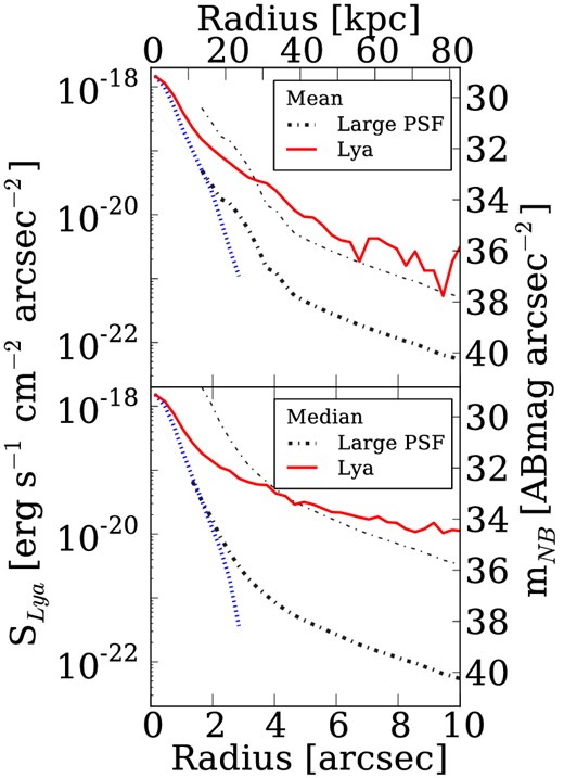
Radial SB profiles of LAEs and PSFs in the Lyα images of NB387. The red solid lines represent the Lyα profiles of LAEs. The blue and black dashed lines denote the small- and large-scale PSFs, respectively. The grey lines are the large-scale PSF profiles with offsets in SB for the shape comparison with the Lyα profiles. Top and bottom panels show the results of mean- and median-combined methods, respectively.
3.2 Tests for all systematic errors
In Section 3.1, we rule out the possibility that the large-scale PSFs give spurious signals mimicking extended Lyα. However, there are a number of unknown systematics that include flat-fielding and sky-subtraction errors. Although the large-scale flat-fielding error may not be a major source of systematics in our high-quality images of Suprime-Cam, one needs to carefully evaluate total errors contributed from all sources of systematics. We carry out image stacking for objects that are not LAEs, which are referred to as non-LAEs. Because non-LAEs have no intrinsically extended emission-line haloes like LAHs, extended profiles of non-LAE composite images should be given by a total of all systematic effects. We thus make composite images of non-LAEs, and investigate how much systematics the total of all systematic errors produce.
First, we randomly choose non-LAEs with the same number as our LAEs. These non-LAEs have size and NB-magnitude distributions same as those of our LAE samples (Fig. 5). To make a Lyα image of the non-LAE sample, we normalize a composite continuum image to match the total flux of a composite NB image, and then subtract the continuum image from the composite NB image. We investigate whether an artificial extended profile appears in the Lyα image of non-LAEs. To reveal uncertainties of this estimate, we repeat it 10 times for 10 realizations. Figs 6 and 7 present composite images of non-LAEs given by the mean- and median-combined methods, respectively. We identify no significant extended profiles in these images. We should note that a ring-like structure found at the source centres of NB387 data is attributable to the slight differences between small-scale PSF profiles of continuum and NB images, which are irrelevant to the extended profiles. Radial profiles of Lyα images of non-LAEs are shown with black lines in Fig. 8. In the NB387 panels of Fig. 8, we find that there are artificial extended profiles at the level of ≲1020 erg s−1 cm−2 arcsec−2, but that these profiles of artefacts are significantly different from those of LAEs in the SB-profile amplitude and shape. These tests confirm that the total of systematic uncertainties do not produce spatially extended profiles similar to the Lyα profiles of LAEs in the NB387 images. Based on these tests, we conclude that the spatially extended profiles of NB387 LAEs in our Lyα images are real, and regard these spatially extended Lyα features as LAHs. Similarly, the panels of NB503 and NB816 show that the differences between profiles between LAEs and artefacts exist clearly, and the LAHs of NB503 and NB816 are also identified. The profile of median-combined image of NB921 is different from that of artefacts in the SB-profile amplitude, but the profile of mean-combined image of NB921 is only beyond that of the artefacts with a small offset. These results indicate that there exist LAHs of NB921 LAEs, although we need to carefully discuss the NB921 results below. In Fig. 8, the extended profiles of NB570 are indistinguishable from those of artefacts. Note that the NB570 data are made of a small number of observation image frames, and that the quality of NB570 data is not as good as the other NB images (Ouchi et al. 2008). Due to the poor quality of NB570 data, significant signals of extended NB570 profiles beyond the artefacts are probably not identified. We find that the extended profiles of NB570 (z = 3.7) are artefacts, and do not discuss the profiles of z = 3.7 LAEs in the following sections.
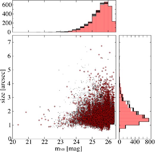
Size and NB-magnitude distribution of LAEs and non-LAEs of NB387 images. In the central panel, the red and black circles represent LAEs and non-LAEs, respectively. Similarly, in the top and right panels, red and black histograms denote LAEs and non-LAEs, respectively.
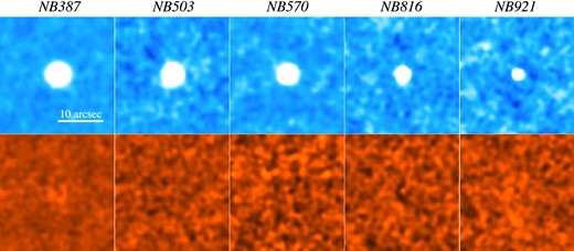
Composite continuum (top panels) and Lyα (bottom panels) images of non-LAEs that are made by the mean-combined method. From left to right panels, we show NB387, NB503, NB570, NB816, and NB921 images.
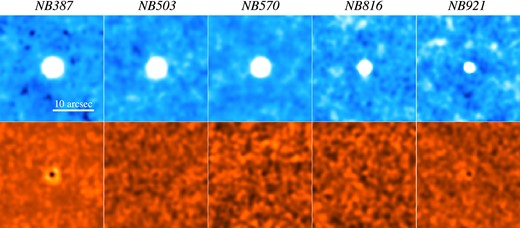
Same as Fig. 6, but for the median-combined method.
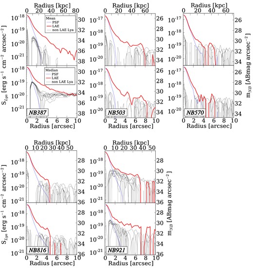
Radial profiles of LAEs, non-LAEs, and PSFs in the Lyα images of NB387, NB503, NB570, NB816, and NB921. The red and black lines represent LAEs and non-LAEs of 10 realizations, respectively. The blue dotted lines denote the small-scale PSFs. Top and bottom panels show the results of mean- and median-combined methods, respectively.
4 RESULTS
In Sections 2 and 3, we have identified LAHs in our Lyα images, and confirmed that the LAH signals are not produced by systematic errors. In this section, we estimate the scalelengths of our LAHs based on the radial profiles of composite Lyα images.
4.1 Definition of the scalelength
4.2 Scalelengths of our LAHs and comparisons
We perform the profile fitting to our LAHs at z = 2.2, 3.1, 5.7, and 6.6, and estimate rn as well as Cn values. Note that the profile fitting results are not presented for our sample of z = 3.7 (i.e. NB570) whose extended profiles are made of artefacts (Section 3.2). All of the LAH-detected samples, except the one of z = 2.2, have similar Lyα luminosity limits of LLyα = 1–3 × 1042 erg s−1. Since our LAE sample of z = 2.2 reaches a Lyα luminosity limit fainter than those of our z ≥ 3.1 samples, we make a subsample of z = 2.2 LAEs with a Lyα luminosity down to 1 × 1042.0 erg s−1 that consists of 2115 LAEs.4 In this way, we obtain samples of LAEs at z = 2.2–6.6 with an average Lyα luminosity limit of LLyα ≳ 2 × 1042.0 erg s−1. Table 1 summarizes our best-fitting parameters and those in the literature. Below, we show details of our results, and compare our results with those from previous studies.
4.2.1 z = 2.2
We find that the best-fitting scalelengths of our LAHs at z = 2.2 are |$r_n=10.0^{+0.38}_{-0.36}$| and |$7.9^{+0.56}_{-0.49}$| kpc (|$14.0^{+9.0}_{-3.9}$| and 11.1|$^{+1.2}_{-0.97}$| kpc) for the entire and subsamples, respectively, which are estimated by the mean-combined (median-combined) method. The SB limits of our composite Lyα images reach depths of 1.3 × 10⁻²⁰ and 1.6 × 10⁻²⁰ erg s−1 cm−2 arcsec−2 in our entire and subsamples, respectively. Steidel et al. (2011) have detected LAHs by stacking NB images of 92 LBGs with a mean spectroscopic redshift of 〈z〉 = 2.65. The scalelengths of the LAHs in Steidel et al. (2011) are rn = 25.2 kpc (mean) and 17.5 kpc (median) which are ∼2 times larger than our values. This discrepancy is probably originated from the difference of galaxy populations, LBGs, and LAEs, and detailed discussions are given in Section 5.3. On the other hand, Feldmeier et al. (2013) have found no extended Lyα emission in their composite image made from 187 LAEs at z = 2.06. The difference between our and Feldmeier et al.'s results is probably due to their SB limit shallower than those of our composite images by one to two orders of magnitudes.
4.2.2 z = 3.1
The best-fitting scalelengths of our z = 3.1 LAHs are |$r_n=9.3^{+0.48}_{-0.53}$| (mean) and |$6.3^{+2.5}_{-1.4}$| kpc (median) down to the SB limit of 1.7 × 10⁻¹⁹ erg s−1 cm−2 arcsec−2. Matsuda et al. (2012) have identified LAHs at z = 3.1 with their large LAE samples, and found that their scalelengths depend on the surface number density of LAEs. The scalelengths obtained by Matsuda et al. (2012) are 9.1 and 20.4 kpc in the LAE's lowest and highest density environments, respectively. The scalelength in the lowest density environment is comparable with our z = 3.1 values within the fitting errors, while the scalelength in the highest density environment is larger than our z = 3.1 values. We revisit this issue of environment in Section 5.3. Feldmeier et al. (2013) have marginally detected LAHs by stacking 241 and 179 LAEs at z = 3.10 and 3.21, respectively. Their scalelengths are rn = 2.8–8.4 kpc, which are also comparable to our scalelengths.
4.2.3 z ≥ 5.7
For our z = 5.7 and 6.6 LAHs, we obtain |$r_n= 5.9^{+0.65}_{-0.53}$| and |$12.6^{+3.3}_{-2.4}$| kpc with the mean-combined data down to the SB limits of 5.5 × 10⁻²⁰ and 1.8 × 10⁻¹⁹ erg s−1 cm−2 arcsec−2, respectively. Similarly, for the median-combined data, the scalelengths of z = 5.7 and 6.6 LAHs are 7.7|$^{+1.9}_{-1.3}$| and 13.9|$^{+0.75}_{-0.99}$| kpc, respectively. There are no previous results that can be compared with these scalelengths of our results. Note that Jiang et al. (2013) have found no LAHs around z = 5.7 and 6.6 LAEs with their small sample of 43 and 40 LAEs, respectively. Although Jiang et al. (2013) claim that their stacked images reach the SB limit of 1.2 × 10⁻¹⁹ erg s−1 cm−2 arcsec−2 at the 1σ level that is comparable to our SB limits within a factor of ∼2, the error estimates are unclear in Jiang et al. (2013). The results of no-LAH detection of Jiang et al. (2013) are probably due to their small statistics.
The results shown above indicate that the scalelengths from the median-combined images are comparable with those from the mean-combined images within the 1σ uncertainties for the most of measurements. We confirm that our results do not significantly depend on the choice of statistics. Moreover, the results are not affected by the contamination of our LAE samples (Section 2), since, under the influence of contamination, the results of mean-combined images should be different from those of median-combined images. Because the median-combined image results include additional uncertainties explained in Section 2.2, we regard the mean-combined image measurements as reliable results. We hereafter make discussions based on the mean-combined image results, unless otherwise specified.
4.3 Size evolution of LAHs
We investigate evolution of LAH scalelengths in the redshift range of z = 2.2–6.6. Fig. 9 presents the scalelengths as a function of redshift. The scalelengths at z = 2.2–5.7 fall in the range of 5–10 kpc that includes measurement uncertainties (Table 1). Thus, Fig. 9 indicates no evolution of the scalelengths from z = 2.2 to 5.7. In the redshift range of z = 5.7–6.6, there is a hint of increase of scalelength. The scalelengths in the mean-combined method increase from z = 5.7 to 6.6 over the fitting errors, |$r_n=5.9^{+0.65}_{-0.53}$| kpc at z = 5.7 and |$r_n=12.6^{+3.3}_{-2.4}$| kpc at z = 6.6. Because, in Section 3.2, we find that the z = 6.6 LAH profile of mean-combined image would be influenced by artefacts, this increase may not be real based on the data of mean-combined images. However, the same trend is also found in the scalelengths obtained by the median-combined method with no signature of artefacts; 7.7|$^{+1.9}_{-1.3}$| and 13.9|$^{+0.75}_{-0.99}$| kpc at z = 5.7 and 6.6, respectively. Thus, our data indicate the increase of scalelength from z = 5.7 to 6.6, although the significance of increase is only beyond the statistical error.
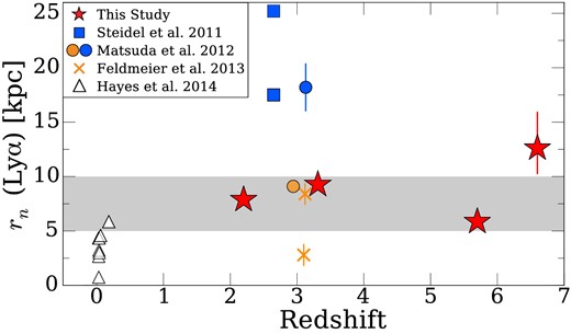
Scalelength as a function of redshift. The red stars represent the scalelengths estimated by the mean-combined method in this study. The grey shade indicates the range of 5–10 kpc in which our reliable scalelength estimates at z = 2.2–5.7 fall. The blue squares and circle denote scalelengths of LAHs found around LBGs of Steidel et al. (2011) and Matsuda et al. (2012), respectively. The orange circle represents the lowest density region LAEs of Matsuda et al. (2012), which are slightly shifted along the abscissa for clarity. The orange crosses are the scalelengths of LAHs around LAEs (Feldmeier et al. 2013). For reference, we plot Lyα Petrosian radii of local LAEs with the open triangles (Hayes et al. 2013, 2014). Here, we regard galaxies with a Lyα equivalent width of ≥20 Å as local LAEs in Hayes et al. (2013, 2014), and plot Petrosian radii of their samples that meet this equivalent-width criterion.
5 DISCUSSIONS
5.1 Do LAHs really exist?
The existence of LAHs around high-redshift galaxies is under debate (Feldmeier et al. 2013; Jiang et al. 2013). In Fig. 3, we identify statistically significant extended Lyα emission around our LAEs at z = 2.2–6.6 based on our unprecedentedly large LAE samples that allow us to achieve ∼10–100 times deeper SB limits than those of typical previous studies (e.g. Steidel et al. 2011; Feldmeier et al. 2013; see Table 1). In Section 3, we examine potential systematic errors that would mimic LAHs, and find that the large-scale PSF of instrumental and atmospheric effects cannot produce radial profiles of our extended Lyα emission in SB and shape (Fig. 4). Besides the large-scale PSF, there are a number of potential systematic effects, such as flat-fielding and sky-subtraction errors (e.g. Feldmeier et al. 2013) as well as unknown systematics. To reveal the total systematic errors involved in our data and analysis, we stack non-LAEs (Fig. 5) in the same manner as our LAEs, and carry out the empirical tests. We find that there exist systematic errors that make an extended emission signal, but that no systematic errors can make a radial profile with the SB amplitude and shape similar to those of our extended Lyα emission of LAEs, except for our sample of z = 3.7 LAEs whose data quality is poor (Fig. 8). Thus, we conclude that we definitively identify LAHs around the LAEs with our data by our analysis technique. Our results indicate that LAEs commonly possess LAHs at z = 2.2–6.6.
5.2 Physical origin of LAHs
In theoretical studies, LAHs are thought to be produced primarily by two physical mechanisms: (1) the resonant scattering of Lyα in the CGM and/or IGM (e.g. Laursen & Sommer-Larsen 2007; Zheng et al. 2011; Dijkstra & Kramer 2012; Jeeson-Daniel et al. 2012; Verhamme et al. 2012) and (2) the cold streams (e.g. Faucher-Giguère et al. 2010; Goerdt et al. 2010; Rosdahl & Blaizot 2012). Our observational results imply that LAHs would be made by the former mechanism.
First, we discuss the possibility of resonant scattering. Lyα photons escaping from a galaxy are scattered by the neutral hydrogen in the CGM within a few 100 kpc from the centre of galaxy, making the Lyα emission extended more than that of stellar continuum. Theoretical predictions indicate that the SB profiles of LAHs are determined by a combination of the ISM dynamics and distribution (e.g. Laursen & Sommer-Larsen 2007; Zheng et al. 2011; Dijkstra & Kramer 2012; Verhamme et al. 2012). Laursen, Razoumov & Sommer-Larsen (2009a) and Laursen, Sommer-Larsen & Andersen (2009b) have carried out Monte Carlo radiative transfer simulations of Lyα propagating through the ISM with various kinematic properties, and found that the extent of LAHs is r ∼ 50–100 kpc. Verhamme et al. (2012) have predicted that the clumpy and inhomogeneous ISM produces an LAH with a characteristic radius of r ∼ 10–20 kpc in their cosmological simulations. The LAHs from our observations also extend up to a radius of r ∼ 30–80 kpc similar to those of the simulations (Fig. 3). Moreover, similar LAHs are predicted for the neutral IGM scattering Lyα photons at the epoch of reionization (e.g. Zheng et al. 2011; Jeeson-Daniel et al. 2012). Thus, the sizes of observed LAHs are comparable to those of Lyα scattering models, which indicate that the major physical origin of the LAH is probably the resonant scattering of Lyα photons in neutral hydrogen of the CGM and/or IGM.
Secondly, we examine whether the cold streams would be a major mechanism of the LAH formation. Cosmological hydrodynamic simulations have predicted that high-redshift (z ≥ 2) galaxies assemble baryon via accretion of relatively dense and cold gas (∼104 K) that represents the cold streams (e.g. Kereš et al. 2005; Dekel et al. 2009a,b). At the temperature of ∼104 K, the cold gas could primarily emit Lyα (e.g. Fardal et al. 2001), which would produce an LAH around galaxies (Faucher-Giguère et al. 2010; Goerdt et al. 2010; Rosdahl & Blaizot 2012). Cosmological simulations have predicted that Lyα emission are more extended for a higher dark halo mass of host galaxies. Rosdahl & Blaizot (2012) have found that cold streams in dark haloes with a mass of ≥1012 M⊙ produce extended Lyα structures, but that Lyα emission is centrally concentrated (<20 kpc in diameter) in less massive dark haloes with a mass of ∼1011 M⊙. Because the typical dark halo mass of LAEs is estimated to be ∼1011±1 M⊙ (Ouchi et al. 2010 and reference therein), the cold streams would not make an LAH as large as 30–80 kpc found in our data. The cold streams are probably not the major mechanism of the LAH formation.
5.3 Scalelength dependence on galaxy population and environment
In Section 4.2, we find differences of scalelengths between measurements of this and some previous studies.
First, at z ∼ 2, the scalelengths from this study are smaller than those from Steidel et al. (2011) by a factor of ∼2 (Fig. 9). Note that the scalelengths of Steidel et al. (2011) are estimated for their LBGs, while our study obtains the scalelengths of LAEs. By definition, Lyα emission of LAEs are brighter than that of LBGs, at a given SFR or UV continuum on average. Theoretical studies suggest that the resonance line of Lyα can escape from galaxies with a low column density of neutral hydrogen in the CGM (Zheng et al. 2011; Verhamme et al. 2012). This physical picture of Lyα escape is confirmed by recent imaging and spectroscopic observations (Shibuya et al. 2014a,b). Based on this picture, Lyα photons produced in star-forming regions of LAEs reach the observer with little resonant scattering. The observer thus finds that Lyα profiles of LAEs are more centrally concentrated than those of LBGs, and obtains a bright Lyα luminosity in the central core of Lyα profile of LAEs above the shallow detection limit of non-stacked images. On the other hand, LBGs have more resonant scattering in the CGM than LAEs, and Lyα profiles of LBGs are largely extended. This is consistent with the fact that the SB of LBGs of Steidel et al. (2011, ∼10−18 erg s−1 cm−2 Hz−1 arcsec−2 at 30 kpc) is one order of magnitude brighter than that of our LAEs (∼10−19 erg s−1 cm−2 Hz−1 arcsec−2 at 30 kpc). The scalelength difference between our LAEs and Steidel et al.'s LBGs indicates that LAEs do not have much neutral hydrogen CGM that scatters Lyα, and that the Lyα profiles of LAEs are steeper than LBGs.
Secondly, at z ∼ 3, the LAH scalelengths of our LAEs are comparable with those of the lowest density environment LAEs of Matsuda et al. (2012), but lower than the highest density environment LAEs of Matsuda et al. (2012, Fig. 9). Here, the galaxy populations of our and Matsuda et al.'s samples are the same. The difference between scalelengths is probably explained by the environment. Clustering analysis with our LAE samples indicates that our survey field at z = 3.1 is not a high-density region (Ouchi et al. 2008, 2010). Our results confirm that low-density environment LAEs have a moderately small scalelength of rn ≃ 5–10 kpc, and support the idea of the environmental effect on LAHs that is claimed by Matsuda et al. (2012). Theoretical studies have predicted that the SB profiles are affected by the galaxy environment. Zheng et al. (2011) have found that the SB profiles of their LAHs at z = 5.7 have three notable features separated at two radial positions; a central cusp at r ≤ 0.2 Mpc (comoving), a relatively flat part at r ∼ 0.2–1 Mpc, and an outer steep region at r ≥ 1 Mpc. The two radial positions of r = 0.2 and 1 Mpc are characterized by the one- and two-halo terms of dark matter haloes. However, we do not find such features in the radial profiles of our LAHs. This is probably because our LAHs at z = 5.7 are only found within an inner region of r ≤ 0.2 Mpc, and/or the clustering strength of the SXDS field is weaker than that of Zheng et al. (private communication). One needs deeper images than those of this study to investigate the environmental effect at the moderately high redshift of z = 5.7.
5.4 Size evolution of LAHs
We find no size evolution of LAHs (rn ≃ 5–10 kpc) from z = 2.2 to 5.7 as we describe in Section 4.3. Malhotra et al. (2012) have measured the half-light radii of stellar distribution of LAEs, rc, in the rest-frame UV, and found no size evolution (rc ∼ 1 kpc on average) in the redshift range of z ≃ 2–6. These two results indicate that the size ratio of LAHs to stellar component is almost constant, rn/rc ∼ 5–10, between z = 2.2 and 5.7. This ratio is comparable with those of z ∼ 2 LBGs (rn/rc ∼ 5–10; Steidel et al. 2011) and z ∼ 0–3 LAEs (rn/rc ∼ 2–4; Matsuda et al. 2012; Hayes et al. 2013). The former LBG results indicate that there is a scaling relation between the LAH and stellar-distribution sizes over the samples of LBGs and LAEs. The latter should be comparable, because these results include a low-density environment LAE sample similar to ours. This no evolution of rn and rn/rc at z = 2.2–5.7 is interesting, because similar trends of no evolution of LAE's physical properties are found in this redshift range. Spectral energy distribution fitting of our LAE samples have revealed that stellar population of our LAEs do not evolve significantly in the redshift range of z = 2.2–5.7 (Ono et al. 2010a,b; Nakajima et al. 2012, see also Gawiser et al. 2006b; Pentericci et al. 2007, 2010; Finkelstein et al. 2011; Malhotra et al. 2012). Moreover, hosting dark haloes of LAEs are typically of masses MDH = 1011±1 M⊙ at z = 2–7 (Ouchi et al. 2010 and reference therein), and do not evolve. These observational results of no evolution of rn, rn/rc, stellar population, and dark halo mass would indicate that LAEs are the population in a specific stage of galaxy evolution, which NB observations can snapshot.
We find a possible increase of scalelength from z = 5.7 to 6.6 in Section 4.3 (see Fig. 9). Again, clustering analysis with our LAEs indicates that our survey field at z = 6.6 is not a high-density region (Ouchi et al. 2010), and it is unlikely that this increase is due to the environmental effect. Because there is no significant increase of scalelengths in the redshift range of z = 2.2–5.7, this sudden increase from z = 5.7 to 6.6 may be explained by cosmic reionization. Signatures of the increase in the neutral hydrogen fraction of IGM (|$x_{{\rm H\,\small {I}}}$|) at z ≥ 7 have been found by many observational studies based on Lyα luminosity functions of LAEs or the Gunn–Perterson test of QSOs (e.g. Fan et al. 2006; Ota et al. 2008; Ouchi et al. 2010; Goto et al. 2011; Kashikawa et al. 2011; Shibuya et al. 2012). Numerical simulations show that Lyα emission around star-forming galaxies is extended due to the neutral hydrogen in the IGM (e.g. Zheng et al. 2011; Jeeson-Daniel et al. 2012). Jeeson-Daniel et al. (2012) have predicted that the SB profile of LAHs becomes flatter in the IGM with a high |$x_{{\rm H\,\small {i}}}$|. The relatively large scalelength of our LAHs at z = 6.6 may come from a more neutral IGM at the epoch of reionization, although the reliability of increase is not very high in statistics (Fig. 9) and systematics (Section 3.2; see Section 4.3 for the details). To conclude this trend, one needs a large amount of high-quality NB data such as obtained by the upcoming survey of Subaru Hyper Suprime-Cam (HSC).
6 SUMMARY
We investigate diffuse LAHs of LAEs with composite Subaru NB images of (3556, 316, 100, 397, 119) LAEs at z = (2.2, 3.1, 3.7, 5.7, 6.6), and discuss their physical origin and size evolution. The major results of our study are summarized below.
We detect extended Lyα emission around LAEs at z = 2.2–6.6 in the composite images. We carefully examine whether the radial profiles of Lyα emission can be made by systematic errors that include a large-scale PSF of instrumental and atmospheric effects. Stacking Lyα images of randomly selected non-LAEs, we confirm that the combination of all systematic errors cannot produce the extended Lyα emission in our composite images of all redshifts of z = 2.2–6.6, except for z = 3.7 whose data have a quality poorer than the others. We thus conclude that the extended Lyα emission found in our composite images are real, and regard the extended Lyα emission as LAHs.
We investigate radial SB profiles of our LAHs, and measure their characteristic exponential scalelengths. The scalelengths are estimated to be ≃ 5–10 kpc at z = 3.1–5.7 and 12.6|$^{+3.3}_{-2.4}$| kpc at z = 6.6 for LAE samples with LLyα ≳ 2 × 1042 erg s−1 (Fig. 9 and Table 1). The comparison with the LAH scalelengths given by previous LBG and LAE studies would indicate that the radial profiles of LAHs depend on galaxy populations and environment: LAEs have a centrally concentrated Lyα profile, and LAEs in low-density regions possess less extended LAHs.
We identify no evolution of scalelengths (5–10 kpc) from z = 2.2 to 5.7 beyond our measurement uncertainties. Combining with no size evolution of LAHs and UV-continuum emission of LAEs found by Malhotra et al. (2012, rc ∼ 1 kpc) over z ∼ 2–6, we suggest the ratio of rn/rc to be nearly constant (rn/rc ∼ 5–10) over the redshift range z = 2.2–5.7. This no evolution of rn/rc probably indicates that the population of LAEs at z = 2.2–5.7 would be in the same evolutionary stage.
We find a possible increase in the scalelength from z = 5.7 to 6.6. This sudden increase only found at z > 6 may be a signature of increasing neutral hydrogen of IGM that scatters Lyα photons due to the cosmic reionization. This finding would support the theoretical model predictions (Jeeson-Daniel et al. 2012), although there remain the possible problems of statistical and systematic effects on the measurements of rn at z = 6.6. The upcoming surveys such with Subaru HSC will allow us to test whether this hint of increase is real or not.
We thank Alex Hagen, Caryl Gronwall, Lucia Guaita, Yuichi Matsuda, Michael Rauch, James Rhoads, Anne Verhamme, and Zheng Zheng for useful comments and discussions. This work was supported by World Premier International Research Center Initiative (WPI Initiative), MEXT, Japan, and KAKENHI (23244025) Grant-in-Aid for Scientific Research (A) through Japan Society for the Promotion of Science (JSPS). KN and SY acknowledge the JSPS Research Fellowship for Young Scientists.
By this reason, the results from the mean-combined images are thought to be more reliable than those from the median-combined images (Section 4.2).
The PSF size of all images is matched to 1.32 arcsec in FWHM by the image smoothing described in (i).
The FWHM PSF size is 1.32 arcsec given by the image smoothing in Section 2.2. The smoothing makes the data points strongly correlated each other within the scale of 1.32. arcsec
Our profile fitting is carried out both for the entire sample and subsample of z = 2.2 LAEs.
