


Abstract
We have carried out continuum and line polarization observations of two protoplanetary nebulae (PPNe), CRL 618 and OH 231.8+4.2, using the Submillimeter Array in its compact configuration. The frequency range of observations, 330–345 GHz, includes the CO(J = 3→2) line emission. CRL 618 and OH 231.8+4.2 show quadrupolar and bipolar optical lobes, respectively, surrounded by a dusty envelope reminiscent of their asymptotic giant branch phase. We report a detection of dust continuum polarized emission in both PPNe above 4σ but no molecular line polarization detection above a 3σ limit. OH 231.8+4.2 is slightly more polarized on average than CRL 618 with a mean fractional polarization of 4.3 and 0.3 per cent, respectively. This agrees with the previous finding that silicate dust shows higher polarization than carbonaceous dust. In both objects, an anticorrelation between the fractional polarization and the intensity is observed. Neither PPNe shows a well-defined toroidal equatorial field, rather the field is generally well aligned and organized along the polar direction. This is clearly seen in CRL 618 while in the case of OH 231.8+4.2, the geometry indicates an X-shaped structure coinciding overall with a dipole/polar configuration. However in the later case, the presence of a fragmented and weak toroidal field should not be discarded. Finally, in both PPNe, we observed that the well-organized magnetic field is parallel with the major axis of the 12CO outflow. This alignment could indicate the presence of a magnetic outflow launching mechanism. Based on our new high-resolution data we propose two scenarios to explain the evolution of the magnetic field in evolved stars.
INTRODUCTION
Protoplanetary nebulae (PPNe) are the by-products of low- and intermediate-mass stars (∼0.8–8 M⊙) in transition between the asymptotic giant branch (AGB) and the planetary nebula (PN) phases. At this stage of stellar evolution the central star is not hot enough to fully ionize the still present circumstellar envelope. PPNe therefore have massive molecular and dust shells, relics of past-AGB mass-loss events (Kwok 1993). Consequently observational studies based on the thermal emission of the dust continuum and molecular species have been conducted over the years at submillimetre, millimetre and centimetre wavelengths (e.g. Sánchez Contreras et al. 1998; Woods et al. 2005; Bujarrabal et al. 2012). These studies revealed the properties of the dust grains and molecules, the distribution and geometry of the material and the kinematics of the molecular and dusty winds (leading in some cases to the discovery of fast, i.e. ≥100 km s−1, outflows).
In contrast, the polarization of both the dust continuum and molecular lines is still poorly studied. The polarimetric information at these longer wavelengths is primarily used to trace the magnetic field's geometry and to study anisotropy in the envelope; it also yields information on the dust grains properties (e.g. nature, size). Submm-to-cm polarimetric investigations are then important tools for the understanding of PPNe.
Dust continuum polarization is based on the principle of alignment of non-spherical spinning dust grains with their long axis (and therefore the polarization angle) perpendicular to the magnetic field (Lazarian 2003; Lazarian & Hoang 2011). The linearly polarized emission of these grains therefore gives a direct image of the magnetic field distribution/geometry by rotating the polarization vectors by 90°. It is important to notice however that this process is generally valid for simple and constant field geometry at different scales (Matthews, Wilson & Fiege 2001; Matthews, Fiege & Moriarty-Schieven 2002).
Former investigations at submillimetre wavelengths based on this mechanism include especially the work of Hildebrand, Dragovan & Novak (1984) and Hildebrand (1996, and references therein) on star-forming regions and molecular clouds. Only two studies exploiting dust continuum polarization/alignment, and focusing on evolved stars (i.e. PNe and PPNe) have been published and these included only one PPN. In particular, Greaves (2002) and Sabin, Zijlstra & Greaves (2007) both targeted CRL 2688 and showed the presence of linearly polarized dust emission at 450 and 850 μm in the nebular envelope using the submillimetre instrument Submillimetre Common-User Bolometer Array (SCUBA) on the James Clark Maxwell Telescope (JCMT). These studies revealed a complex magnetic field structure with what appeared to be a combination of toroidal and poloidal fields.
In the case of molecular lines1 the Goldreich–Kylafis effect (Goldreich & Kylafis 1981, 1982) predicts that the emission from rotating molecules can be polarized (in the order of a few per cent) in the presence of a magnetic field. The polarization occurs when anisotropic radiation alters the molecular magnetic sublevels. Morris, Lucas & Omont (1985) proposed another explanation and linked the polarization to a stellar radiation field resulting in a preferential rotational direction for the molecules. The latter hypothesis does not necessarily imply the action of magnetic fields. However contrary to the case of dust polarization, emission-line polarization vectors can be either parallel or perpendicular to the magnetic field. The polarization direction will be strongly affected by the physical conditions within the objects (e.g. radiation field, hydrogen number density, magnetic field). Few evolved objects have been investigated using their polarized molecular lines and the most recent papers focused on AGB stars such as IRC +10216 (Girart et al. 2012) and IK Tau (Vlemmings et al. 2012). PPNe have not yet been studied using this method.
The combination of both dust and molecular polarization is a valuable tool to determine the magnetic field geometry and anisotropy in PPNe. We present such a dual polarimetric study on the circumstellar envelopes of two well-known PPNe: CRL 618 and OH 231.8+4.2.
CRL 618 (also named the Westbrook Nebula) is a ∼200 yr old (Kwok & Bignell 1984) PPN located at ∼0.9 kpc (Goodrich 1991; Sánchez Contreras & Sahai 2004). The nebula is characterized by two pairs of shocked, rapidly expanding lobes (Balick et al. 2013), belonging to the ‘multipolar’ morphological class following Sahai et al. (2007), a central compact H ii region and an ancient AGB halo (Sánchez Contreras, Sahai & Gil de Paz 2002). CRL 618 is also known for its rich carbonaceous dust and molecular content which have been extensively studied at submillimetre, millimetre and centimetre wavelengths from ground based to space telescopes (Phillips et al. 1992; Nakashima et al. 2007; Bujarrabal et al. 2010; Tafoya et al. 2013).
OH 231.8+4.2 (also known as the Rotten Egg Nebula or Calabash Nebula) is a slightly older PPN (≃770 yr; Alcolea et al. 2001) with a bipolar morphology as illustrated by its two asymmetrical elongated lobes. Similar to CRL 618, the PPN displays an external round halo. The nebula is located at ≃1.12 or 1.30 kpc according to Choi et al. (2012) and Kastner et al. (1992), respectively, and shelters a binary star system [main sequence A-type + Mira (QX Pup) following Sánchez Contreras, Gil de Paz & Sahai 2004a. OH 231.8+4.2 has a rich molecular spectrum and an oxygen-rich chemistry, although carbonaceous species such as HCN, HNC and CS are also seen (Morris et al. 1987). This PPN has therefore been widely studied from far-infrared (IR) to radio wavelengths by e.g. Morris et al. (1987), Sánchez Contreras et al. (1997) and Alcolea et al. (2001). Its magnetic field has been studied by Etoka et al. (2009) and Leal-Ferreira et al. (2012, 2013) using OH and H2O masers, respectively. The latter authors derived a magnetic field of ≃45 mG which extrapolated to the stellar surface and assuming a toroidal field configuration gives a field of ≃1.5–2.0 G. Etoka et al. (2009) derived a radial field along the outflow. We note that maser studies provide very high spatial resolution but sparse sampling, and less information on large scales.
Our submillimetre investigation is organized as follows. In Section 2 we describe the observations and data reduction. Section 3 includes the continuum polarization results for CRL 618 and OH 231.8+4.2, respectively, followed by the line polarization results. Finally, the discussion and concluding remarks are presented in Sections 4 and 5, respectively.
OBSERVATIONS AND DATA REDUCTION
We observed CRL 618 and OH 231.8+4.2 with the Submillimeter Array (SMA)2 (Ho, Moran & Lo 2004) in polarimetric mode (Rao & Marrone 2005). We used the compact configuration giving a maximum baseline of ≃77 m. The selected frequency range is divided between the lower side band (LSB; ≃330–334 GHz) and the upper side band (USB; ≃342–346 GHz). These ranges were chosen to also cover the CO lines in the J = 3→2 transition, i.e. 13CO and 12CO, at rest frequencies 330.587 and 345.796 GHz, respectively.
The correlator set-up provides a spectral resolution of ∼0.8 MHz (i.e. 0.70 km s−1) at 345.796 GHz. 3C 111 was used as gain calibrator and 3C 279 as a bandpass and polarization calibrator for both objects. CRL 618 was observed on 2011 November 28 for ≃16 h (including the calibrators) with a telescope phase centre |$\alpha _{{\rm J2000}}={\rm 04^{h} 42^{m} 53 {.\!\!^{{\mathrm{s}}}}64}$|, δJ2000 = +36°06′53|${^{\prime\prime}_{.}}$|4. The weather conditions were excellent with a mean zenith τ of 0.045 at 225 GHz and stable phases during the observations. OH 231.8+4.2 was observed on 2011 December 27 for ≃14 h (including the calibrators) with a telescope phase centre |$\alpha _{{\rm J2000}}={\rm 07^{h} 42^{m} 16 {.\!\!^{{\mathrm{s}}}}83}$|, δJ2000 = −14°42′52|${^{\prime\prime}_{.}}$|1. The weather conditions were not optimal due to snow at the summit. The mean τ was 0.075 (the maximum value reached was 0.13) and the phases were also unstable during the observing run.
The flux, gain and bandpass calibration were performed with the software mir3 and then exported to miriad (Wright & Sault 1993; Sault, Teuben & Wright 2011) for polarization calibration and imaging. Our data were corrected for polarization leakage (i.e. instrumental polarization); we found for both objects consistent leakage terms of ≃5 per cent in the lower sideband and ≃2 per cent in the upper sideband consistent for both objects. We also emphasize that a strong polarization calibrator such as 3C 279 coupled with a good coverage of parallactic angle results in an accuracy of 0.1 per cent in instrumental calibration (Marrone & Rao 2008).
RESULTS AND ANALYSIS
The high resolution provided by the SMA allows us to identify different line splitting in both objects which are likely linked to velocity motions as well as the large expansion of the 12CO(J = 3–2) molecular line in CRL 618 indicating a fast CO outflow.
Continuum polarization
CRL 618
The continuum was carefully selected and subtracted from both the LSB and USB avoiding the inclusion of emission lines such as the relatively strong CO(J = 3–2), CS(J = 7–6), H13CN(J = 4–3), HC3N(J = 38–37) by visually examining the visibility amplitude spectra. The final maps of the thermal continuum emission in CRL 618 (relative to dust polarization and magnetic fields) were made combining the line-free channels of the USB and LSB. To obtain the best sensitivity for the Stokes I (total intensity) and Stokes Q and U (linear polarization), we used a robust weighting (in order to minimize the noise level) resulting in a synthesized beam of 2.2 × 1.9 arcsec2 with a position angle (PA) of −77| $_{.}^{\circ}$|6. The measured rms noise levels, σI = 19.8 mJy beam−1 and σQ, U = 2.2 mJy beam−1, defined the zero levels we applied to establish the polarization maps. The polarized intensity and percentage of polarization [IP and P(per cent), respectively] are defined as the following: |$I^{2}_{\rm P}=Q^{2}+ U^{2} - \sigma ^{2}_{Q,U}$| and P(per cent) = IP/I (with I the total intensity).
The continuum dust emission was detected over an area of approximately 5.4 ×4.6 arcsec2 centred at the coordinates |$\alpha ={\rm 04^{h} 42^{m} 53 {.\!\!^{{\mathrm{s}}}}582}$|, δ = +36°06′53|${^{\prime\prime}_{.}}$|40 (Fig. 1, top). The continuum emission is slightly elongated east–west and this is consistent with the results by Martin-Pintado et al. (1993, although at higher angular resolution). The measured peak intensity, located in the dark lane of the PPN, is 3.4 Jy beam−1 with a mean of 1.2 Jy beam−1 over the full area of the continuum emission.
![Hα images of CRL 618 (top) and OH 231.8+4.2 (bottom) from the Hubble Space Telescope with their respective dust continuum emission [(red contours in steps of ∼3σ × (0.5, 1, 2, 3, 4, 5, 6, 7, 8, 9)] from the SMA observations, superimposed. Both PPNe show a clear asymmetry and the submm emission is roughly elongated in the direction of the outflows (see more details in the text). The positional offset of the continuum peak and (0, 0) position is stated in Sections 2 and 3 for both objects. North is up and east is left in all frames.](https://oup.silverchair-cdn.com/oup/backfile/Content_public/Journal/mnras/438/2/10.1093_mnras_stt2318/2/m_stt2318fig1.jpeg?Expires=1749185576&Signature=1YEj2wEk1fwMPCtBFLJrl57WtjDtgOuaRhYIbPO2y-GiKZDQqax9gRLu47Pi29NE94lIFwulQo6cvZ4MDVmRNmA~MDQW9lux72J1Nk494g4Yc2Bupl09QF0O6zG9cU8vJzCWzDV7hm7~IPH6x8EF8kfzZkAZ9bl2avsfVIqsutD7hGKwqK05Bm-yfg32V920sbLQ6lCAs~D3xY08-JTiKdKFNhszVc6JBmb~cmXZdd2J3FsxHItKS68VImPGWMqRfBNqgO60bn~SqbFRaJTQDkCpTsc~h0fW~OThesUoDKQEFejvedzZ-DA9IkaDdBpqRGQGlv1nzyQF8Cx9zUDyMw__&Key-Pair-Id=APKAIE5G5CRDK6RD3PGA)
Hα images of CRL 618 (top) and OH 231.8+4.2 (bottom) from the Hubble Space Telescope with their respective dust continuum emission [(red contours in steps of ∼3σ × (0.5, 1, 2, 3, 4, 5, 6, 7, 8, 9)] from the SMA observations, superimposed. Both PPNe show a clear asymmetry and the submm emission is roughly elongated in the direction of the outflows (see more details in the text). The positional offset of the continuum peak and (0, 0) position is stated in Sections 2 and 3 for both objects. North is up and east is left in all frames.
Linear polarization is detected above ≃3σ across the source. The polarimetric information obtained reveals a peak of 9.6 mJy beam−1 (at |$\alpha ={\rm 04^{h} 42^{m} 53 {.\!\!^{{\mathrm{s}}}}621}$|, δ = +36°06′53|${^{\prime\prime}_{.}}$|79) and a mean polarized emission of 7.0 mJy beam−1 which correspond to 4.4σ and 3.2σ detections, respectively. The peak continuum intensity is not coincident with the peak fractional polarization P(per cent) = 0.7. However, the mean polarization over the whole structure is quite low with P(per cent) = 0.3. Those values depend on the assumed zero level (derived from the noise level), but we do not expect it to reach values greater than ∼1 per cent. The polarization vectors can be divided in two main sets which overall form a slightly curved pattern opening towards the east (Fig. 2, left). The first set is linked to the upper (northern) half of the polarized continuum and shows a mean polarization angle of ≃22°; the second set is linked to the lower (southern) half of the polarized continuum and shows a mean polarization angle of ≃–10°. We however have to be careful while discussing the variation in polarization angle as the polarization emission is not spatially resolved, as shown by the size of synthesized beam. Assuming that the magnetic field direction is given by rotating the dust polarization vectors, in Fig. 2, left, by 90°, we obtain the magnetic map in Fig. 2, right which we discuss later in this paper (Section 4).
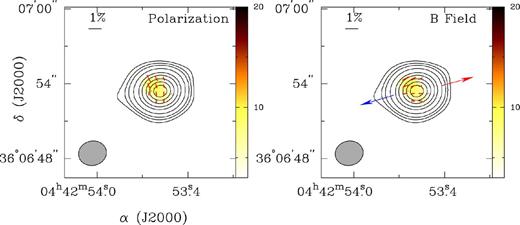
Left: combined (USB+LSB) polarization map of CRL 618. Right: combined magnetic field map derived by rotating the polarization vectors by 90°. The magnetic field vectors show a geometry which can be linked to a polar field distribution mostly aligned (in the centre) with the outflows indicated by the arrows. The red and blue correspond to the red- and blueshifted CO outflow (see Fig. 8 later). In both cases, the black contours which indicate the total dust emission are drawn in steps of 0.02 Jy × (3, 6, 10, 20, 40, 60, 90, 120, 150). The colour image indicates the polarized intensity with its associated scale bar in Jy beam−1 on the right. Finally, the polarization vectors are drawn as red segments and the scale is set to 1 per cent. The segments are greater than 2.5σ detections with the peak value of 4.4σ. The uncertainty in PA due to thermal noise is about 5°. North is up and east is left. In all maps the polarization segments were slightly oversampled when exporting the data from miriad–cgdisp display tool to the interactive graphics software wip (Morgan 1995).
OH 231.8+4.2
The robust weighting applied resulted in a synthesized beam of ≃2.5 × 1.9 arcsec2 with a PA of −11| $_{.}^{\circ}$|1. The rms noise derived for the Stokes I, Q and U was σI = 20.5 mJy beam−1 and σQ, U = 4 mJy beam−1. The thermal emission from the continuum appears as an elongated distribution extending over an area of ≃7.3 × 5.7 arcsec2 and centred at the coordinates |$\alpha = {\rm 07^{h} 42^{m} 16 {.\!\!^{{\mathrm{s}}}}979}$|, δ = −14°42′49|${^{\prime\prime}_{.}}$|70 (Fig. 1, bottom). The peak intensity (located at the coordinates |$\alpha = {\rm 07^{h} 42^{m} 16 {.\!\!^{{\mathrm{s}}}}955}$|, δ = −14°42′49|${^{\prime\prime}_{.}}$|77) is 0.78 Jy beam−1 with a mean of 0.31 Jy beam−1 over the whole area. The polarized structure in OH 231.8+4.2 strongly differs from that of CRL 618 as it appears fragmented into four parts (Fig. 3, left). The largest component (≃2 × 1.5 arcsec2) is located in the north-east section and shows a peak polarized intensity of 16 mJy beam−1 (≃4σ; which is not exactly coincident with the peak of Stokes I) and a mean polarized intensity of 11 mJy beam−1 (≃2.7σ) is measured over this polarized area. The south-east component shows a similar polarized intensity of ≃16 mJy beam−1 (mean of 11 mJy beam−1) and this is the location of the strong peak percentage of polarization with a value of ≃15.6 per cent (the mean percentage is 6.7 and 4.3 per cent over the whole structure). The north-west and south-west components both show polarized intensities of ∼10 mJy beam−1 with a mean of ∼9 mJy beam−1. We highlight a slight east–west gradient in the polarized intensity distribution. The intervening positions between the four regions do not have polarization detection above 2.5σ (which is the cut-off in Stokes Q and U when computing polarization angles for OH 231). The repartition of the electric vectors is also quite interesting as each component presents not only well-organized patterns but also a main PA with values and signs different from the immediate neighbour. Indeed, the north-east and north-west spots have global PAs of approximately −34°± 18° and +57°± 3°, respectively, the south-east and south-west spots show global PAs of +70°± 3° and −8°± 5°, respectively. The derived magnetic field map (Fig. 3, right) is different than that of CRL 618 due to the fragmented detected polarized emission (see discussion in Section 4).
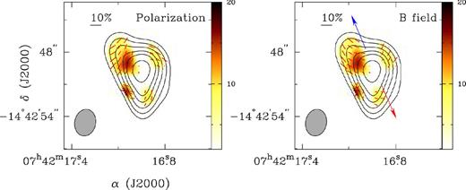
Same as Fig. 2 but for OH 231.8+4.2. Left: combined (USB+LSB) polarization map. The continuum contours are drawn in steps of 0.02 Jy × (3, 6, 10, 15, 20, 30, 40, 50, 60). Right: combined magnetic field map with the polarization vectors rotated by 90°. The field's structure shows an X-shaped (or dipole) configuration. Similarly to CRL 618 the arrows indicate the direction of the (blue- and redshifted CO) outflows. The polarization vectors are drawn as red segments and the scale is set to 10 per cent.
Spectral line polarization
In an attempt to detect molecular line polarization we also targeted the strongest molecular lines present in both objects: 13CO(J = 3→2) in the LSB and 12CO(J = 3→2) in the USB. The SMA spectra are shown in Figs 4 and 5 for CRL 618 and OH 231.8+4.2, respectively. We note that recently, Lee et al. (2013a) presented a higher resolution (∼0.3 and ∼0.5 arcsec) spectrum as well as high-resolution maps, of CRL 618 at 345 GHz also using the SMA, although they do not cover our full spectral range.
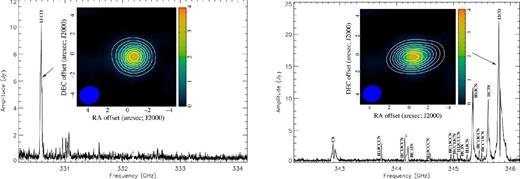
LSB (left) and USB (right) visibility amplitude spectra of CRL 618. The emission is averaged over all SMA baselines. The red arrow indicates the 32 MHz coverage gap width. We show for each spectrum the geometry of the integrated emission of the CO lines (contours) over the continuum (colour) as well as some well identified emission lines. Line splitting is seen in the CS and 12CO lines. The contours are set as steps of (2, 3, 4, 5, 6, 7, 8, 9) × 32.9 Jy beam−1 (km s−1)−1 in the LSB map and ×139.3 Jy beam−1 (km s−1)−1 in the USB map.
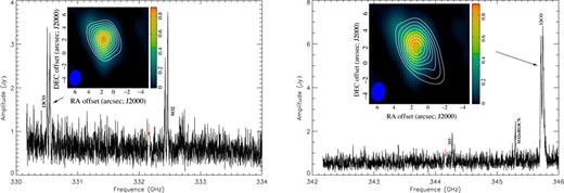
Same as Fig. 4 but for OH 231.8+4.2. The spectra are quite noisy (compared to CRL 618 and due to the wet weather) with the LSB being noisier than the USB as expected. The high resolution provided by the SMA allows us to identify different line splitting for the 13CO, SO2 and 12CO lines (in both objects), which are likely linked to velocity motions as well as the large expansion of the molecular lines. Thus, in the case of the 12CO(3→2) line, the splitting is indicating of a fast CO outflow. For each spectrum we emphasize the distribution of the integrated emission of the CO lines (contours) over the continuum (colour). The contours are set as steps of (2, 3, 4, 5, 6, 7, 8, 9) × 27.3 Jy beam−1 (km s−1)−1 in the LSB map and ×39.5 Jy beam−1 (km s−1)−1 in the USB map.
The noise in the (Stokes Q and U) emission line is higher than that of the continuum, requiring a higher zero-level to assert the presence of polarization. The analysis of those lines did not return any detection above 3σ and therefore any conclusive signs of polarization. However the percentage of polarization is not expected to be high and we estimate an upper limit between 5 and 10 per cent. Indeed, as previously mentioned, similar investigations by Girart et al. (2012) and Vlemmings et al. (2012) obtained detectable polarization at sigma levels greater than ∼4–5 in the AGB stars IRC +10216 and IK Tau. In those cases the maximum polarization fraction varied from ≃2 up to ≃13 per cent for the different lines observed in both objects (SiS 19–18, CS 7–6, CO 3–2, CO 2–1 and SiO 5–4).
DISCUSSION
The SMA data obtained indicate the presence of a polarized continuum at submillimetre wavelengths in the PPNe CRL 618 and OH 231.8+4.2. Several observations can be made regarding the dust polarization in these objects and the magnetic field geometry.
Grain dust properties
We observed that OH 231.8+4.2 is more polarized on average, in terms of degree of polarization, than CRL 618 despite its non-uniform coverage. Thus, the mean degree of polarization in CRL 618 is 0.3 and 4.3 per cent for OH 231.8+4.2. Both objects differ in their chemistry, and Sabin et al. (2007) have shown that in their sample, and at the same wavelength, the mean degree of polarization of the oxygen-rich PNe/PPNe is greater than that of the carbon-rich PNe/PPNe. The two new nebulae studied here also follow this trend. This supports the idea that the grain alignment efficiency is higher in O-rich than in C-rich envelopes and therefore dust chemistry plays a role not only in the polarization process but also in our interpretation of magnetic field distribution.
Carbon grains have generally a smaller size than silicate grains and may not produce significant polarization.4 Also, it would be easier or more likely for larger grains to host superparamagnetic particles (Jones & Spitzer 1967; Mathis 1986; Kim & Martin 1993), such as iron or magnetite, which would cause a higher level of polarization and a more efficient dust grain alignment by the magnetic field. The polarized intensity appears to be sensitive to the grain shape as well (Kim & Martin 1995) and most of the dust alignment theories require either elongated (e.g. oblate/prolate spheroids) or irregular grains (Lazarian 2003). Therefore one would expect that the presence in the disc of OH 231.8+4.2 of larger grains with iron inclusions, crystalline olivine (MgFeSiO4), crystalline enstatite (MgSiO3) and H2O crystalline ices (Maldoni et al. 2004, via modelling), would produce a greater polarization than CRL 618, which presents carbonaceous dust (mostly amorphous carbon; see Lequeux & Jourdain de Muizon 1990).
Unfortunately a detailed study of the dust grain properties in those objects is still missing.
Depolarization effect
An anticorrelation is seen between the fractional polarization and the total intensity in both objects. Indeed, P(per cent) tends to decrease from the edges to the centre of the emission area, opposite to Stokes I. This ‘depolarization effect’ is not new and has often been observed in dark clouds, molecular clouds and starforming regions (e.g. Chen et al. 2012) but also, and most relevant here, in PNe and post-AGBs (Greaves 2002; Sabin et al. 2007). This pattern can be associated with multiple phenomena such as the effect of beam smearing, a complex magnetic field distribution (Matthews et al. 2001; Greaves 2002) and a loss of efficiency in the grain alignment (Lazarian, Goodman & Myers 1997) due to molecular collisions or the variation of the density which would alter the structure of the dust grains and therefore the degree of alignment (Cho & Lazarian 2005).
Dust distribution
As previously mentioned the polarization indicates the location of aligned dust. In both PPNe this polarized dust is circumscribed inside the optical dark lane.
In CRL 618 the polarized grains are roughly perpendicular to the direction of the ionized outflows (Fig. 2, left). The emission, expanding over ≃3.8 arcsec2, might be related to the dusty torus/ring or to the central bipolar compact H ii region (Kwok & Bignell 1984;5 Sánchez Contreras & Sahai 2004, see their fig. 6).
In OH 231.8+4.2 the polarization vectors, which are divided into four groups, indicate different polarization angles and seem to draw the contours of a dusty region (if we link them all) which might also delimit a ring or torus of ≃3.6 arcsec radius well centred on the equator of the PPN (Fig. 3, left). This distribution appears consistent with the ring-like structure described by the polarization vectors associated with the OH masers in Etoka et al. (2009).
Magnetic field distribution
The magnetic field in CRL 618 is globally aligned with the pairs of ionized outflows (indicated by the arrows in Fig. 2, right). Indeed the polarization vectors of the main structure show a mean PA of ≃96° while the PPN has a mean PA along the lobes of ≃94°. The orientation of the magnetic field is mostly at 90°to the equatorial plane of CRL 618. This configuration is pretty similar to the structure of CRL 2688, which is another carbon-rich PPN with exactly the same optical quadrupolar morphology. CRL 618 therefore shows a well-defined polar magnetic field. The magnetic field appears to be well organized.
The field's distribution in OH 231.8+4.2 is particularly patchy. The eastern side of the PPN (also showing the higher polarization intensity) presents in each small area a very well organized curved field directed away from the equatorial plane (Fig. 3, right). The magnetic vectors describe at first sight an X-shape which would then associate the magnetic field in OH 231.8+4.2 with a dipole configuration (see model by Padovani et al. 2012). However, we cannot discard another interpretation that is the low inclination respected to the equatorial plane of some vectors belonging to the north-west and south-east blobs (and to some extent the south-west blob), might indicate the presence of a partial (and not strongly delineated) toroidal field. OH 231.8+4.2 would in this case show a dual configuration such as the PPN CRL 2688.
It is interesting to notice that neither of these two high-mass nebulae shows a well defined and constrained toroidal equatorial magnetic field such those seen in the PNe NGC 6537, NGC 6302 and NGC 7027, which in turn show no poloidal field (Sabin et al. 2007). But they coincide more with the magnetic distribution of CRL 2688 where the field is mainly aligned with the polar direction. CRL 618, OH 231.8+4.2 and CRL 2688 being younger than the ‘NGC group’, we may see here a correlation with the evolutionary stage of the nebulae. This would then indicate that there is a tendency for the distribution of the magnetic field to evolve from a single dipole/poloidal configuration to a toroidal one (passing through a phase of dual configuration) while the nebulae evolve (Fig. 6, panel a). This type of transition generally occurs via the mechanism of rotation. An alternative is that both configurations might exist simultaneously (Fig. 6, panel b). In this case we postulate that the initially weak toroidal field (as it is often the case in slow rotator objects) could co-exist with a stronger poloidal one. As the nebula expands, the later declines quickly, as r−2, respective to the toroidal field which begins to dominate because it declines as r−1. This would explain why no poloidal configuration is seen in more evolved nebulae e.g. PNe (see also Gardiner & Frank 2001).
A greater statistical sample and a multiscale analysis of the magnetic field distribution are still needed to answer the ‘evolutionary problem’.
So how do magnetic fields account for the bipolar or multipolar shapes observed? As we observed non-spherical geometry before the occurrence of the toroidal fields the latter cannot be the main dynamically shaping agent, i.e. with enough energy to constrain the material in the equatorial plane and launch collimated outflows. However, it has been theoretically claimed that dipole magnetic fields can as well lead to non-spherical geometry. For instance, Matt et al. (2000) have shown that a dipole field could create a dense equatorial torus and collimate the winds (with no need of a companion star). The newly created aspherical geometry would then be conserved and/or enhanced with the evolution towards a toroidal field.
Taking into account all the recent works arguing for the major role played by close binary systems in the shaping of PPNe/PNe (e.g. Soker 2004; Nordhaus 2008; Douchin et al. 2013; Tocknell, De Marco & Wardle 2013), a plausible scheme would involve a rotational effect induced by binary interaction which then would have some dynamical effects on the formation and evolution of the magnetic field and on the objects’ morphologies.
Molecular outflows and launching mechanism
The study of the emission lines in both PPNe can help us to investigate the relationship between the outflows and the magnetic field. In both objects we note the relatively strong and high velocity of the CO outflows6 and as the 12CO(J = 3→2) line is the most significant in terms of intensity we will then consider that the molecular outflows are mainly supported by this emission line. Figs 4 and 7, top, show the CO molecular outflows for CRL 618 while Figs 5 and 7, bottom, show the same but for OH 231.8+4.2.
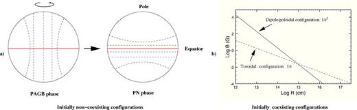
Sketches illustrating the possible evolutionary scenarios of the magnetic field in evolved stars. On the left, we show the full change in magnetic configuration, i.e. from a dipole/poloidal to a toroidal (via rotation). The dashed lines indicate the magnetic field lines. Detailed toroidal, dipole and quadrupole magnetic field geometries (from modelling) have also been presented by Padovani et al. (2012) and by Matt et al. (2000). On the right, we present an adaptation of the graphic by Vlemmings (2011) showing the variation of the magnetic field strength in function of the stellar radius and according to the magnetic field configuration (i.e. dipole/polar and toroidal). Assuming that both configurations co-exist from the beginning, it is clear that the dipole field will disappear first and faster, leaving a dominant toroidal field.

12CO channel maps for CRL 618 (top) and OH 231.8+4.2 (bottom). The contours are set at 10 per cent of the peak. In the channel maps, the peak of the continuum is represented by the star symbol and the velocity in km s−1 is indicated in the top right-hand corner. Both sets of maps indicate the presence of high-velocity gas in the PPNe.
A good positional correlation between the continuum area and the 12CO emission in CRL 618 is seen in Fig. 4. The comparison of the direction of the well-organized magnetic field vectors with that of the overall CO molecular outflows in Fig. 8 , left, shows that they are well aligned.
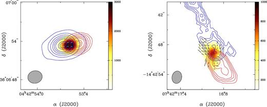
Distribution of the 12CO(J = 3→2) outflow versus the magnetic field. Left-hand panel: the blue- and redshifted lobes of the 12CO emission in CRL 618 are drawn in contours starting at 10 per cent and in steps of 10 per cent of the peak (blue peak = 828 Jy × km s−1; red peak = 399 Jy × km s−1). The CO outflows are integrated over a velocity range of −110 to −20 km s−1 for the blueshifted lobe and +5 to +90 km s−1 for the redshifted lobe. We can therefore see the integrated emission intensity for each element. The two lobes are aligned with the continuum (Stokes I) emission (colour scale in mJy) and a good agreement is also observed with the magnetic vectors distribution (cyan segments). Right-hand panel: same as the left-hand panel but for OH 231.8+4.2. In this case, the 12CO emission contours start at 30 per cent and in steps of 10 per cent of the peak (blue peak = 100 Jy × km s−1; red peak = 158 Jy × km s−1). The CO outflows are integrated over a velocity range of −60 to +15 km s−1 for the blueshifted lobe and +50 to +110 km s−1 for the redshifted lobe. We observed an elongated blue shifted CO emission and a good correlation between the magnetic vectors (black segments) and the general outflow distributions.
Concerning OH 231.8+4.2, Fig. 5 indicates a slight misalignment of the continuum area with respect to the 12CO emission distribution of ∼30°. Fig. 8, right, shows that the X-shaped (or pinched waist) structure of the magnetic field in OH 231.8+4.2, mostly the northern and eastern segments, encompasses quite well the blue- and redshifted lobes of the 12CO emission. The magnetic vectors in OH 231.8+4.2 are globally parallel to the CO molecular distribution and trace quite well the outer contours of the red- and blueshifted CO lobes.
In both cases the alignment between the major axis of the molecular outflows and the ordered magnetic field suggests not only a dynamically important field at small scale but could also indicate the presence of a magnetic launching mechanism of these outflows. Our observations are concordant with the theoretical predictions by Blackman et al. (2001) relative to the presence of a poloidal geometry of the magnetic field at small distance from the central star and its role in the launching of the flows in PPNe. Recently, Pérez-Sánchez et al. (2013) have also reported the radio observation of a magnetically collimated outflow/jet shaping the post-AGB star IRAS 15445−5449. However, we cannot discard the possibility of a field dragged by the powerful outflows, particularly in the case of OH 231.8+4.2. Investigations at larger depths, i.e. closer to the central star, are however needed to fully assert the hypothesis outflow launching theory.
Magnetic field strength
An estimate of the field strength can however be obtained via maser observations and Zeeman splitting analysis. Table 1 summarizes the different studies using this method related to CRL 618 and OH 231.8+4.2. It is worth mentioning that these masers are located in the outer layers of the envelopes and are therefore not very reliable for a global field estimation.
Summary of masers study in CRL 618 and OH 231.8+4.2.
| PPN | Maser type | B-field strength | Field configuration | B-field extrapolation | Reference |
|---|---|---|---|---|---|
| CRL 618 | CN (N = 1–0) | 0.9 G(a) | Toroidal(b): r−1 | 200 G(a) at 8 R⋆ | Herpin et al. (2009) |
| 2 kG(a) at 1 R⋆ | |||||
| OH 231.8+4.2 | OH | – | Poloidal and Toroidal | – | Etoka et al. (2009) |
| H2O | 45 mG | Toroidal(b): r−1 | ≃2.5 G at 1 R⋆ | Leal-Ferreira et al. (2012) |
Note. Contrary to the other studies where Zeeman splitting was used to measure the field's strength, Etoka et al. (2009) analysed the distribution of the 1667 MHz OH masers and observed, similar to our study, a well organized magnetic field with a partial orientation of the field along the outflows.
aUpper limit.
bAssumed field configuration.
By determining the ratio β between the thermal pressure Pth = nHkT and the magnetic pressure PB = B2/8π we can estimate the lower limit on the magnetic field's strength for which the field would become dominant. Bujarrabal et al. (2002) provided a detailed analysis of OH 231.8+4.2 and its physical conditions and following their work we calculate that in the dense central part of the PPN where T = 35 K and nH = 3 × 106 cm−3, the magnetic pressure dominates for B ≥ 0.6 mG. This threshold indicates that, assuming Leal-Ferreira et al. (2012)'s result, the magnetic pressure largely dominates the thermal pressure at this location in this PPN.7 Similarly, based on the work by Sánchez Contreras et al. (2004b) in the dense core of CRL 618 (T = 55 K and nH = 7.5 × 106 cm−3), the magnetic pressure dominates for B ≥ 1.2 mG, a value much lower than that found by Herpin et al. (2009). Although we estimated upper limits on the magnetic field for the molecular (neutral) areas in both PPNe (with low temperatures and high densities), the ionized regions (with higher temperatures) should not be discarded as the field still needs a partial ionization to connect to the gas. Indeed in the outflows (showing high kinetic energy), the magnetic field might not govern the gas flow. We are therefore likely to see a variation of the flow–field relation inside the PPN.
CONCLUSIONS
In this paper we present high-resolution SMA submillimetre polarimetric observations of the PPNe CRL 618 and OH 231.8+4.2. In both cases we detected linear polarization above ∼3σ and a higher percentage polarization is found in CRL 618 (C-rich) compared to OH 231.8+4.2 (O-rich). The difference is likely to be linked to the chemical nature (i.e. dust grain type) of the PPNe as also reported by Sabin et al. (2007) for other evolved objects.
Furthermore, the polarization vectors indicate that the resulting magnetic field geometry supports the presence of a clear and well organized poloidal magnetic structure (i.e. aligned with the pairs of ionized outflows) in both PPNe. But while this configuration is more ‘simple’ in CRL 618; the field shows an X-shaped structure in OH 231.8+4.2 and appears particularly patchy (although the field is organized in each individual component). However we do not discard the possibility that some vectors might belong to a toroidal field.
The observation of polarization in the molecular lines, and particularly the CO lines, led to no positive detections above 3σ in any of the PPN but we clearly observed, in both cases, an alignment of the ionized and molecular outflows with the magnetic field vectors, at large and small scales, respectively, which supports the idea of a dynamically important field at small scale and of a probable magnetic launching origin for these outflows.
Finally, we present a tentative explanation for the field's configuration evolution in late-type stellar objects.
The SMA probed to be an excellent tool to study the polarization and magnetic field distribution in evolved stars. A better understanding of the role and evolution of magnetic fields in the late stages of stellar evolution will require more of these submillimetre and millimetre observations to investigate any evolutionary scheme or magnetic launching mechanism. In the future with the more sensitive polarization capabilities of Atacama Large Millimeter/Submillimeter Array (ALMA), we will be able to target a larger range of evolved objects particularly the faint PPNe and PNe.
The authors thank the SMA personal for supporting the observations as well as the referee for comments and suggestions, which significantly contributed to improving the quality of the publication. LS also thanks S. Kemp for going through the paper and raising some issues. LS is supported by the CONACYT grant CB-2011-01-0168078, and RV is supported by PAPIIT-DGAPA-UNAM grant IN107914. This research has also made use of the SIMBAD data base, operated at CDS, Strasbourg, France and the NASA's Astrophysics Data System. We acknowledge the use of observations made with the NASA/ESA Hubble Space Telescope, obtained from the data archive at the Space Telescope Science Institute (STScI). STScI is operated by the Association of Universities for Research in Astronomy, Inc., under NASA contract NAS 5-26555.
Excluding masers.
The Submillimeter Array is a joint project between the Smithsonian Astrophysical Observatory and the Academia Sinica Institute of Astronomy and Astrophysics, and is funded by the Smithsonian Institution and the Academia Sinica.
Note that they found a rather small radio core structure of ∼0.3 arcsec major axis.
See also the recent paper by Lee et al. (2013b) for CRL 618.
Note: water masers may come from denser condensations. They commonly show stronger field strength perhaps related to higher local densities.
