


Abstract
The increasing precision in the determination of the Hubble parameter has reached a per cent level at which large-scale cosmic flows induced by inhomogeneities of the matter distribution become non-negligible. Here, we use large-scale cosmological N-body simulations to study statistical properties of the local Hubble parameter as measured by local observers. We show that the distribution of the local Hubble parameter depends not only on the scale of inhomogeneities, but also on how one defines the positions of observers in the cosmic web and what reference frame is used. Observers located in random dark matter haloes measure on average lower expansion rates than those at random positions in space or in the centres of cosmic voids, and this effect is stronger from the halo rest frames compared to the cosmic microwave background (CMB) rest frame. We compare the predictions for the local Hubble parameter with observational constraints based on Type Ia supernova (SNIa) and CMB observations. Due to cosmic variance, for observers located in random haloes we show that the Hubble constant determined from nearby SNIa may differ from that measured from the CMB by ±0.8 per cent at 1σ statistical significance. This scatter is too small to significantly alleviate a recently claimed discrepancy between current measurements assuming a flat Λ cold dark matter (ΛCDM) model. However, for observers located in the centres of the largest voids permitted by the standard ΛCDM model, we find that Hubble constant measurements from SNIa would be biased high by 5 per cent, rendering this tension non-existent in this extreme case.
INTRODUCTION
The Hubble constant is arguably the most fundamental cosmological parameter. It is not only a measure of the expansion rate of the Universe, but it also sets the normalization of the cosmic density parameters. Since the pioneering work by Edwin Hubble, all efforts made to determine this constant have been focused on improving the precision of distance measurements in the cosmic distance ladder as well as on reducing a number of systematic effects, related e.g. with the astrophysics of Cepheids and Type Ia supernova (SNIa; for a review see Freedman & Madore 2010). These efforts have been enabled by the increasing amount and quality of the data, and resulted in measurements of the Hubble constant to an unprecedented per cent level of precision (Riess et al. 2011; Freedman et al. 2012; Tully et al. 2013).
The most competitive methods for the determination of the Hubble constant utilize combined measurements of distances to nearby Cepheids and SNIa, or cosmic microwave background (CMB) observations, although it is worth noting the growing relevance of constraints from time delays between gravitationally lensed multiple images of distant quasars (see e.g. Paraficz & Hjorth 2010; Suyu et al. 2013). The most recent measurement based on SNIa yields H0 = 73.8 ± 2.4 km s−1 Mpc−1 (Riess et al. 2011). On the other hand, assuming a flat Λ cold dark matter (ΛCDM) cosmology a recent analysis of the CMB data from the Planck mission leads to H0 = 67.88 ± 0.77 km s−1 Mpc−1 (Planck Collaboration 2013), which differs from the previous result by 2.4σ (although both measurements seem more compatible, when using the revised determination of H0 from SNIa, based on an improved distance calibration; see Efstathiou 2013). This raises the question to what degree this discrepancy is due to as yet unknown systematic uncertainties or large-scale inhomogeneities (Marra et al. 2013). A similar problem concerns the difference in the expansion rate found between low- and high-redshift supernovae. The Hubble constant determined from SNIa within 75 h−1 Mpc was measured to be 6.5 ± 1.8 per cent higher than that at larger distances (Jha, Riess & Kirshner 2007). This effect, referred to as the Hubble bubble, is commonly ascribed to our location in an underdense region of the cosmic web (Zehavi et al. 1998), although alternative solutions such as reddening of local SNIa were also suggested (Conley et al. 2007). Most recent analyses of SNIa data reveal that a bulk flow of nearby SNIa prevails up to redshift z ≈ 0.06, which corresponds to a comoving distance of 180 h−1 Mpc (Colin et al. 2011; Feindt et al. 2013). It is worth noting that this scale of the bulk flow appears to coincide with the size of a plausible local underdensity determined from galaxy counts in the near-infrared (Keenan et al. 2012; Whitbourn & Shanks 2013).
The determination of the Hubble constant from measurements of distances and recessional velocities in the local Universe is inevitably affected by large-scale flows resulting from fluctuations in the matter distribution (Courtois et al. 2013). It is crucial then to theoretically predict these effects at the level of precision required by upcoming observations. Current theoretical works rely on analytical calculations based on either linear perturbation theory or its modifications that include some non-linear effects (Wang, Spergel & Turner 1998; Cooray & Caldwell 2006; Marra et al. 2013). Although this approach can give valid initial insights, it is insufficient for taking into account all non-linear effects and therefore to provide accurate predictions for the next generation measurements. Non-linear effects not only modify peculiar velocities at small scales, but they also implicitly define locations of reference observers in the most evolved structures of the cosmic web, i.e. dark matter (DM) haloes. The only way to include all these effects in a theoretical calculation of the variance of the perturbed Hubble flow is to use cosmological N-body simulations (Turner, Cen & Ostriker 1992; Martinez-Vaquero et al. 2009). In this paper, we utilize large-scale cosmological N-body simulations to study the effects of large-scale inhomogeneities and the distribution of DM haloes on the local measurements of the Hubble constant. The simulations were run in volumes comparable to the Hubble volume, and thus they are suitable for a statistical study on the local Hubble flow. The goal of the paper is not only to quantify deviations of the local Hubble parameter from the global expansion rate, but also to consider a number of assumptions, such as the location of reference observers in the cosmic web or the reference frame for the measurement, which considerably modify these predictions.
The manuscript is organized as follows. In Section 2, we describe the simulations and methods used to find DM haloes and cosmic voids. In the next section, we introduce the notion of the local Hubble parameter and its connection to large-scale inhomogeneities. We also describe here the technical details of calculating predictions for the local Hubble parameter based on cosmological simulations. Section 4 presents the main results of the paper and is divided into several detailed subsections in which the effects of different sets of assumptions to calculate the local Hubble parameter are discussed. In Section 5, we calculate the theoretical predictions for a few different measurements of the Hubble parameter based on SNIa or CMB data and compare them to observational constraints. We conclude and summarize in Section 6.
SIMULATIONS
We use two large-scale cosmological N-body simulations, the JUropa HuBbLE volumE1 (Jubilee, Watson et al. 2013) with a volume of (6 h−1 Gpc)3 and a part of the Big MultiDark (Big MD; Heß et al., in preparation) which is a suite of simulations with volumes of (2.5 h−1 Gpc)3. The two simulations are based on the results of the of 5 yr CMB data from the Wilkinson Microwave Anisotropy Probe (WMAP) satellite (Dunkley et al. 2009; Komatsu et al. 2009). The assumed cosmological parameters, (Ωm = 0.27, ΩΛ = 0.73, Ωb = 0.044, h = 0.70, σ8 = 0.80, ns = 0.96) for the Jubilee and (Ωm = 0.29, ΩΛ = 0.71, Ωb = 0.047, h = 0.70, σ8 = 0.82, ns = 0.95) for the MD, are consistent with recent results from Planck (Planck Collaboration 2013). For more details of each simulation see Watson et al. (2013) and Heß et al. (in preparation).
The two simulations have 60003 (Jubilee) and 38403 (Big MD) particles. The corresponding particles masses are 7.49 × 10¹⁰ h−1 M⊙ and 2.2 × 10¹⁰ h−1 M⊙, yielding minimum resolved halo masses (with 50 particles) of 4 × 10¹² and 1 × 10¹² h−1 M⊙, respectively. Combining the two simulations, we resolve DM haloes spanning the mass range from Milky Way-size galaxies with 1012 h−1 M⊙ to massive galaxy clusters with 1015 h−1 M⊙.
DM haloes in both simulations are found using the amiga halo finder, ahf (Gill, Knebe & Gibson 2004; Knollmann & Knebe 2009). The finder identifies the halo centres as the overdensity peaks located on a recursively refined grid. Every centre is then used to find gravitationally bound particles and, on the basis of these particles, to calculate various properties of the haloes, including the halo mass Mhalo which is defined as the mass of a spherical overdensity region with the mean density equal to 178ρb, where ρb is the background density. The final sets of all distinct haloes identified in the Jubilee and the Big MD simulations (both at redshift z = 0) contain 9.1 × 10⁷ haloes with masses Mhalo > 1013 h−1 M⊙ and 5.8 × 10⁷ haloes with masses Mhalo > 1012 h−1 M⊙, respectively. For the latter, there are 5 × 10⁷ haloes with masses 1012 h−1 M⊙ < Mhalo < 1013 h−1 M⊙.
In addition to DM haloes, we also identify voids formed in the Jubilee simulation. Voids are found as regions in the simulation box which do not contain DM haloes above a certain mass (Watson et al. 2013). We adopt 1014 h−1 M⊙ as the mass threshold of the void finder. With this mass limit, we identify the most extended voids which have the strongest effect on the local Hubble parameter. Every void is defined as a sphere that maximally fills a volume devoid of haloes (Gottlöber et al. 2003). The centre of this sphere is used as the void centre. The total number of voids found at redshift z = 0 in the 6 h−1 Gpc simulation is 2.6 × 10⁵.
LOCAL HUBBLE PARAMETER FROM SIMULATIONS
The observed velocities of galaxies in the local Universe combine a recessional velocity component due to the global expansion of the Universe and a peculiar velocity component resulting from the local density fluctuations. Without prior information on the distances to galaxies, these two velocity components cannot be disentangled, and therefore local measurements of the Hubble constant may differ from the actual global rate of expansion. The local Hubble parameter depends not only on the cosmological model, but also on the location of the observer in the cosmic web and on the selection of the objects used for the measurement. A deviation from the global expansion rate is expected on distances which are comparable in size or smaller than cosmic voids, which set a natural scale of transition to homogeneity (Scrimgeour et al. 2012). To study the effects of inhomogeneities on the local Hubble parameter, cosmological simulations should be run in boxes much larger than the largest cosmic structures, i.e. cosmic voids. Depending on the threshold for the density contrast, the effective radii of voids (the radii of spheres with enclosed volumes equal to the volumes of voids) span the range from 10 to 100 h−1 Mpc (Watson et al. 2013). Due to asphericity, maximum sizes of these objects are even a few times larger than the effective radii. Therefore, the side length of the simulation box should be at least of a few h−1 Gpc.
The probability p(observer) should encompass a priori information about our own location in the cosmic web, such as that we live in a galaxy group within a DM halo of a certain mass. This kind of information can significantly modify the final predictions for Hloc. The probability distribution p(observer) may also be interpreted as a mathematical representation of the Copernican principle or any deviation from it. It is a way of quantifying the meaning of the term ‘typical observers’. From a technical point of view, we shall not deal with any explicit form of p(observer), but instead we shall consider different schemes for placing random observers in the cosmic web. Every scheme, however, corresponds to a unique form of p(observer).
In order to calculate p(Hloc) from the simulations, we define a set of observers and haloes hosting observable objects in the Universe, i.e. galaxies and groups of galaxies. In all cases, we use 105 observers which are randomly distributed in the cosmic web according to different choices for p(observer). We checked that the number of observers is sufficient to precisely calculate p(Hloc). For every observer, we find all haloes at distances r < rmax and fit the linear model of equation (1) to the line-of-sight velocities and distances. The resulting 105 best-fitting values of Hloc are then treated as a random sample drawn from the probability distribution p(Hloc). We use these values to compute the mean and the confidence intervals of the probability distribution p(Hloc). We repeat the calculations for the maximum radius rmax spanning the range from 20 to 300 h−1 Mpc. The linear fit is carried out assuming equal weights for all the haloes within rmax so that the final probability distribution of the local Hubble parameter is fully determined by the large-scale structures that emerged from the evolution of the assumed cosmological model. Unless it is explicitly stated (as in Section 4.5), the peculiar velocities in equation (1) are given by the bulk velocities of the haloes in the comoving rest frame. This choice of the reference frame corresponds to measuring the Hubble parameter in the CMB rest frame (Turner et al. 1992). In observations of nearby Cepheids or SNIa, the transformation to this reference frame relies on correcting the observed redshifts for the motion of the Milky Way as determined from the CMB dipole.
When we fit for the local Hubble parameter, we use the peculiar velocities of the haloes in the z = 0 snapshots of the simulations. However, the assumed maximum value of rmax, 300 h−1 Mpc, corresponds to redshift z = 0.1. This means that our calculation neglects the evolution of peculiar velocities at z < 0.1. Using linear perturbation theory (see more details in Section 4.1), we estimate the impact of the evolution between z = 0 and z = 0.1, and find that the resulting relative corrections to the variance of the local Hubble parameter are smaller than 5 per cent. We also check that the corrections needed to account for the differences in cosmological parameters of the two simulations are of the same order of magnitude. To prevent our results from being affected by these two effects, we provide all our results within a 10 per cent precision.
RESULTS
Here, we consider several choices for p(observer) and calculate the corresponding distribution of Hloc. We explore the following distributions of observers within the simulation box: random in space; random in DM haloes of different masses; in the centres of voids; and in the local rest frames of DM haloes.
Random observers in space
The first simple way of selecting observers is to draw random positions in the simulation box (Turner et al. 1992). In this case, observers are not assigned to the haloes and the resulting distribution of the local Hubble parameter represents a volume weighted statistic, i.e. one assigns equal probabilities to all positions in the simulation box rather than to all distinct haloes. This scheme of distributing observers is less natural than selecting random DM haloes as the locations for observers. However, the main motivation for considering this approach is that the same distribution of observers is implied when using analytical calculations based on perturbation theory (for which there is no prediction for halo formation, and thus all statistical quantities are weighted by volume rather than by haloes). Therefore, the framework considered here allows us to directly compare the results from the simulations to those from analytical calculations (see e.g. Wang et al. 1998; Marra et al. 2013). For fitting the Hubble relation given by equation (1), we use haloes with masses Mhalo > 1013 h−1 Mpc from the 6 h−1 Gpc simulation box.
Fig. 1 shows the confidence intervals of the probability distribution of Hloc with respect to its global value H0 as a function of the maximum radius of observations rmax (red shaded contours). As expected, the measurement of the Hubble parameter converges to H0 at large distances. The relative deviation from the global Hubble flow is as small as 1 per cent within 150 h−1 Mpc. Note also that for rmax < 50 h−1 Mpc the mean value of Hloc/H0 is larger than 1 by a few per cent. This effect results from using a volume-weighted statistic which enhances the contribution of the cosmic outflows inside volume-dominated voids.
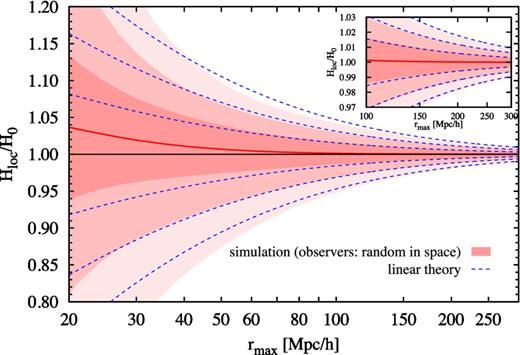
Probability distribution of the local Hubble parameter Hloc within the radius rmax, as measured by observers randomly distributed in space of the 6 h−1 Gpc simulation box (red shaded contours). The red solid line is the mean and the contours are the 68.3, 95.4 and 99.7 per cent confidence intervals. For comparison purposes, the blue dashed contours show the corresponding confidence intervals calculated using linear perturbation theory, with the mean value equal to 1. The inset panel zooms into the main plot for radii rmax > 100 h−1 Mpc.
The blue dashed contours in Fig. 1 show the confidence intervals for a Gaussian probability distribution with the standard deviation given by equation (3) for the same cosmological parameters and power spectrum as used in the simulation. The linear approximation recovers the results from the simulations at scales rmax ≳ 100 h−1 Mpc. Non-linear evolution effects, such as the mean value being larger than 1, become relevant at scales corresponding to typical sizes of voids, i.e. rmax ≲ 40 h−1 Mpc. As shown by Marra et al. (2013), the linear approximation can be analytically corrected for the non-linear evolution of cosmic voids by assuming a log-normal probability distribution instead of a Gaussian.
For the various cases presented in this section, Table 1 lists the mean and scatter of the relative difference between the local Hloc and the global H0 Hubble parameter within three maximum radii rmax: 50, 75 and 150 h−1 Mpc. The maximum radius rmax = 75 h−1 Mpc, corresponding to the Hubble velocity czmax = 7500 km s−1, is commonly adopted as the limiting value separating low-z SNIa, whose Hubble diagram is likely to be significantly perturbed by local inhomogeneities (Zehavi et al. 1998; Jha et al. 2007), from high-z ones, which are thought to probe the global expansion of the Universe (Riess et al. 2011).
Mean μ and scatter σ of the relative difference between the local and global expansion rates, i.e. μ = 〈Hloc/H0 − 1〉 and σ = 〈(Hloc/H0 − 1 − μ)2〉1/2. The first and second columns describe the selection of observers and the mass range of the haloes used in the calculation. The remaining columns list the mean and the scatter of (Hloc − H0)/H0 for rmax of 50, 75 and 150 h−1 Mpc, respectively.
| Observers | log10Mhalo( h−1 M⊙) | μ50(per cent) | σ50(per cent) | μ75(per cent) | σ75(per cent) | μ150(per cent) | σ150(per cent) |
|---|---|---|---|---|---|---|---|
| Random in space | >13 | 0.7 | 3.3 | 0.3 | 2.1 | 0.0 | 0.9 |
| Random in haloes | >13 | −1.7 | 4.0 | −0.8 | 2.4 | −0.2 | 0.9 |
| Centres of voids | >13 | 2.5 | 2.5 | 1.0 | 1.8 | 0.1 | 0.9 |
| Random in haloes | (12, 13) | −0.6 | 3.3 | −0.3 | 2.1 | 0.0 | 0.9 |
| Random in space | No haloes/linear model | 0.0 | 3.5 | 0.0 | 2.2 | 0.0 | 0.9 |
| Random in haloes/halo rest frame | >13 | −3.9 | 4.7 | −1.9 | 2.7 | −0.4 | 1.0 |
Observers in random haloes
The most natural way of distributing observers in the cosmic web is by positioning them in random DM haloes. This scheme assumes that typical observers are located in structures which are embedded in DM haloes, i.e. galaxies or groups of galaxies, such as our own location in the Local Group. This substantially decreases the effective volume of space populated by observers. In this scheme, observers tend to occupy overdense regions and thus their measurement of the Hubble constant is mostly affected by large-scale infall.
Fig. 2 shows the confidence intervals for the local Hubble parameter as measured by observers located in randomly selected DM haloes with masses Mhalo > 1013 h−1 M⊙ in the 6 h−1 Gpc simulation (red shaded contours). The same minimum mass of 1013 h−1 M⊙ is assumed for haloes used in fitting the linear Hubble relation. These results are compared to the previous case for observers randomly distributed space (blue dashed contours corresponding to the red shaded contours in Fig. 1).
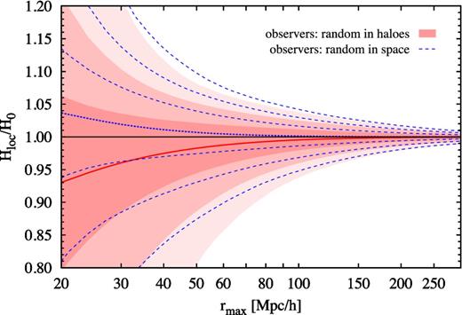
Probability distribution of the local Hubble parameter Hloc within the radius rmax, as measured by observers randomly distributed in DM haloes from the 6 h−1 Gpc simulation box (red shaded contours), and compared to those for the case with observers randomly distributed in space (blue dashed contours). For each case, the contours show the 68.3, 95.4 and 99.7 per cent confidence intervals, whereas the red solid and blue dotted lines show the mean values.
For scales rmax ≲ 70 h−1 Mpc, the distribution of deviations of Hloc from H0 differs significantly from that of the case with observers randomly distributed in space. At these scales, the probability distribution of Hloc is skewed towards smaller values and the mean local Hubble parameter is less than H0. This is due to the fact that observers populate preferentially overdense, infall-dominated regions. The size of the scatter at rmax = 75 h−1 Mpc is comparable to that for observers randomly distributed in space, but the confidence intervals are shifted towards smaller values by 20 per cent of their size. When compared to Fig. 1, it appears that the selection of observers by haloes has a significantly larger effect on the probability distribution of Hloc than the corrections due to non-linear evolution effects for observers randomly distributed in space.
Observers in the centres of voids
The motivation for considering the centres of voids as the locations for the observers comes from observations of SNIa. The Hubble constant appears to be slightly larger at small compared to large distances (Zehavi et al. 1998; Jha et al. 2007). This trend of the Hubble parameter with the distance, referred to as the Hubble bubble, is statistically significant and is commonly ascribed to a local void. The location of the Local Group in a void leads to another choice of the prior probability p(observer): observers located in voids. Here, we consider a rather extreme possibility and locate the observers in the centres of voids.
We use voids from the 6 h−1 Gpc simulation that are identified as regions devoid of haloes with masses Mhalo > 1014 h−1 M⊙. The total number of voids is of the same order of magnitude as the adopted number of observers, i.e. 105. Fig. 3 shows the confidence intervals of the resulting probability distribution of Hloc as a function of rmax (red shaded contours), compared to the results for observers randomly distributed in space (blue dashed contours). From this figure, one can see that for observers located in voids the local Hubble parameter is affected by large-scale outflow. For this case, the mean value of Hloc decreases from 1.06H0 at rmax = 20 h−1 Mpc to 1.01H0 at rmax = 75 h−1 Mpc. Note also that the confidence intervals here are more similar to those for the case with observers randomly distributed in space rather than in DM haloes. This shows how strong the contribution from voids is for a volume-weighted statistic of the local Hubble parameter.
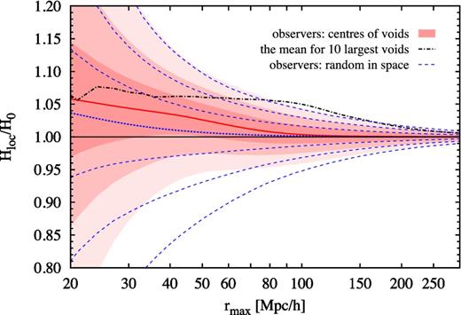
Probability distribution of the local Hubble parameter Hloc within the radius rmax, as measured by observers located in the centres of voids found in the 6 h−1 Gpc simulation box (red shaded contours), and compared to those for the case with observers randomly distributed in space (blue dashed contours). For each case, the contours show the 68.3, 95.4 and 99.7 per cent confidence intervals, whereas the red solid and blue dotted lines show the mean values. The black dash–dotted line shows instead the mean values obtained when only the centres of the 10 largest voids (in terms of the size) are used.
As the most extreme example, we also plot the mean local Hubble parameter as measured with respect to the centres of the 10 largest voids selected by size, with radii between 90 and 100 h−1 Mpc (black dash–dotted line). In this case, the mean of Hloc is ∼5 per cent larger than H0 within all radii up to ∼100 h−1 Mpc. Then, it drops to ∼1 per cent of H0 within ∼200 h−1 Mpc. At scales between 90 and 150 h−1 Mpc, the local Hubble parameter reaches the upper limit of the 99.7 per cent confidence interval of the probability distribution obtained for observers distributed in the centres of all voids.
Observers in groups or clusters of galaxies
Massive haloes tend to populate denser environments, which are surrounded by large-scale infall. Therefore, when selecting observers by haloes one should consider the dependence on the halo mass. We show this effect by considering haloes with masses 1012 h−1 M⊙ < Mhalo < 1013 h−1 M⊙ from the 2.5 h−1 Gpc simulation box. These haloes correspond to massive galaxies or galaxy groups, with the mass range including the mass of the Local Group estimated at 5 × 10¹² h−1 M⊙ (Li & White 2008; Partridge, Lahav & Hoffman 2013). This halo population may be regarded as a random sample drawn from the most natural prior probability of p(observer) describing observers resembling our location in the local cosmic web (we belong to a group, but not to a cluster). We use the same halo population to both select observers and fit the linear Hubble relation.
Fig. 4 shows the probability distributions of Hloc as measured by observers located in randomly selected Local Group-like haloes, i.e. haloes with masses 1012 h−1 M⊙ < Mhalo < 1013 h−1 M⊙ (blue dashed contours). This distribution is compared to the case for observers located in massive haloes of Mhalo > 1013 h−1 M⊙ from the 6 h−1 Gpc simulation box (red shaded contours, the same as in Fig. 2). It can be seen from this figure that the local Hubble flow is less affected by the large-scale infall when using less massive haloes. As expected, the differences due to halo masses become negligible at large scales. Comparing to Fig. 1, one can see that the confidence intervals of Hloc/H0 at rmax < 75 h−1 Mpc for observers located in less massive haloes are more similar to those obtained with simple analytical calculations based on linear perturbation theory than those for observers in more massive haloes (see also Table 1).
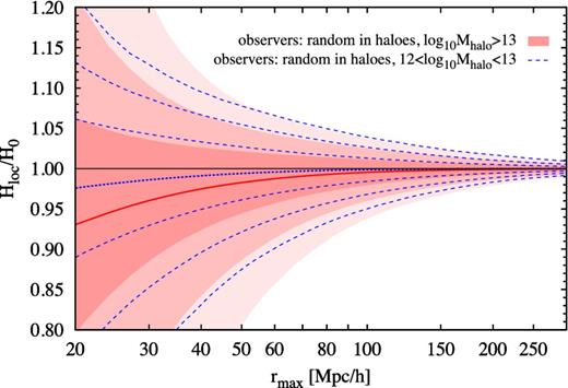
Probability distribution of the local Hubble parameter Hloc within the radius rmax, as measured by observers randomly distributed in DM haloes for two different halo populations: haloes with masses Mhalo > 1013 h−1 M⊙ from the 6 h−1 Gpc simulation box (red shaded contours) and with 1012 h−1 M⊙ < Mhalo < 1013 h−1 M⊙ from the 2.5 h−1 Gpc simulation box (blue dashed contours). For each case, the contours show the 68.3, 95.4 and 99.7 per cent confidence intervals, whereas the red solid and blue dotted lines show the mean values.
Reference frame
Until now, we have assumed that observers are at rest in the comoving coordinate system. This means that the velocities used for fitting the Hubble relation of equation (1) are measured in the CMB rest frame, as in the standard practice of transforming the observed redshifts to the CMB rest frame by using the bulk velocity of the Milky Way as determined from the CMB dipole. Here, we consider a hypothetical situation in which velocities are measured instead in the local rest frames of the haloes.
Fig. 5 compares the predictions for the measurement of the local Hubble parameter in two reference frames: the CMB rest frame (red shaded contours, the same as in Fig. 2) and the local halo rest frames (blue dashed contours). In both cases, observers are located in random haloes with masses Mhalo > 1013 h−1 M⊙ from the 6 h−1 Gpc simulation. The figure shows that the change of reference frame has a significant effect. At scales of rmax ≲ 80 h−1 Mpc, the mean local Hubble parameter measured in the halo rest frames is smaller than the mean determined in the CMB rest frame by 50-70 per cent of the intrinsic scatter. Among all effects summarized in Table 1, the change of the reference frame is the largest.
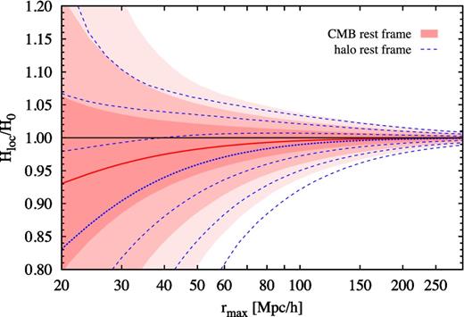
Probability distribution of the local Hubble parameter Hloc within the radius rmax, as measured by observers in the CMB rest frame (red shaded contours) or the local rest frames of DM haloes (blue dashed contours). In both cases, observers are located in random haloes with masses Mhalo > 1013 M⊙ selected from the 6 h−1 Gpc simulation box. The contours show the 68.3, 95.4 and 99.7 per cent confidence intervals, whereas the red solid and blue dotted lines show the mean values.
COMPARISON WITH OBSERVATIONS
We adopt the redshift distributions of three different samples of nearby SNIa used in measurements of the Hubble parameter. The first and second samples were compiled by Jha et al. (2007) and have supernovae at redshifts z < 0.025 and 0.025 < z < 0.10, respectively. These two data sets revealed that the expansion rate of closer supernovae is higher than the rate determined from the distant ones (see also Zehavi et al. 1998). The third sample includes all supernovae from Hicken et al. (2009) at redshifts 0.023 < z < 0.10. This is nearly the same data compilation that was used in the measurement of H0 by Riess et al. (2011).
We calculate the probability distributions of Hloc using the redshift distributions of these three SNIa samples. The reference observers are randomly distributed in DM haloes with masses 1012 h−1 M⊙ < Mhalo < 1013 h−1 M⊙ from the 2.5 h−1 Gpc simulation box and the local Hubble flow is measured in the rest frame of the CMB. Comparison with observational constraints on Hloc can only be made in terms of the relative differences between the Hubble parameters determined from data sets probing Hloc at different scales. Here, we consider two combinations of measurements which have recently attracted considerable attention: (i) the difference in the determination of Hloc between the z < 0.025 and 0.025 < z < 0.10 SNIa samples reported by Jha et al. (2007), and (ii) the difference between the expansion rate determined by using nearby SNIa with an improved distance calibration from Cepheids (Riess et al. 2011) and that by using CMB observations from Planck (Planck Collaboration 2013). In the latter case, we assume that the Hubble constant measured from the CMB is not affected by large-scale structures, i.e. Hloc = H0.
Fig. 6 shows the predicted probability distributions of the relative differences in Hloc for the two combinations of observations (red solid and blue dashed lines, respectively) as well as the corresponding measurements from Jha et al. (2007), 6.5 ± 1.8 per cent, and from combining results from SNIa (Riess et al. 2011) and the CMB (Planck Collaboration 2013), 8.9 ± 3.7 per cent. All quoted errors include only the statistical uncertainties of the measurements.
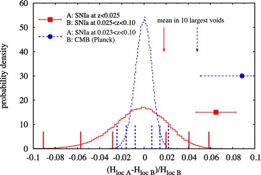
Relative differences in Hloc measured using two sets of observations, A and B, that probe the expansion rate at different scales. The blue point with dashed error bars shows the difference between the expansion rates inferred from SNIa at redshifts z < 0.025 (A) and 0.025 < z < 0.10 (B) from Jha et al. (2007). The red point with solid error bars shows the relative difference between Hloc determined from nearby SNIa at redshifts 0.023 < z < 0.10 (A; Riess et al. 2011) and CMB measurements from Planck (B; Planck Collaboration 2013). The error bars represent only the statistical uncertainties of the measurements. The corresponding lines show the probability distributions of the predicted relative differences in the expansion rate, as measured by observers located in DM haloes with masses 1012 h−1 M⊙ < Mhalo < 1013 h−1 M⊙ formed in a cosmological simulation of a standard ΛCDM model (the 2.5 h−1 Gpc box). The vertical lines indicate the 68.3, 95.4 and 99.7 per cent confidence intervals. The arrows show the mean relative differences in Hloc for observers located in the centres of the 10 largest voids from the 6 h−1 Gpc simulation.
The 3.6σ tension between the expansion rates obtained from nearby (z < 0.025) and distant (0.025 < z < 0.10) SNIa can be easily alleviated by assuming the existence of a local void. For this case, the 99.7 per cent interval of the predicted relative difference in Hloc reaches 5.8 per cent. Taking into account the dispersion of the theoretical distribution in the error budget yields a 2.2σ deviation of the observational results from the predictions of the ΛCDM model assumed here, i.e. 6.9 ± 3.0 per cent (with the mean of the theoretical probability distribution equal to −0.4 per cent).
The effect of cosmic variance is too small to reduce the tension between the value of the Hubble constant determined from nearby SNIa and that from the CMB. The standard deviation of the theoretical probability distribution is 0.8 per cent, which is 30 per cent smaller than the value obtained in analytical calculations by Marra et al. (2013). This value has a negligible effect on the error budget of the relative difference in the expansion rates obtained from SNIa and the CMB, for which the tension remains unchanged at 2.4σ statistical significance (neglecting all systematic errors). We note, however, that this conclusion strongly relies on the assumed prior probability p(observer). Although we chose a very conservative form for p(observer) (random DM haloes with masses comparable to the mass of the Local Group), it is interesting to consider other possibilities. As an extreme example, we recalculate the local Hubble parameter using observers placed in the centres of the 10 largest voids from the 6 h−1 Gpc simulation. The mean relative difference in Hloc from SNIa and the CMB is 4.8 per cent (see the blue arrow in Fig. 6), which accounts for 55 per cent of the measured value and thus decreases the tension between the two measurements to 1σ. On the other hand, the mean relative difference between Hloc from z < 0.025 and 0.025 < z < 0.10 SNIa is 1.6 per cent (see the red arrow in Fig. 6). Such a small value results from the fact that the local Hubble parameter is nearly independent of radius within the range of distances to nearby SNIa (see the black profile in Fig. 3; the median of the distances is 75 h−1 Mpc and the distribution strongly decays at larger radii).
SUMMARY AND CONCLUSIONS
We made use of large-scale cosmological N-body simulations to study the effects of inhomogeneities and the distribution of DM haloes on the measurement of the local Hubble parameter, Hloc. We find that the probability distribution of Hloc depends not only on the peculiar velocity field resulting from inhomogeneities in the matter distribution of a given cosmological model, but also on the distribution of observers used as a prior for the calculation, and on the reference frame of the measurement.
For observers randomly distributed in space, the local Hubble parameter is preferentially larger than the global expansion rate. This happens due to an uneven volume distribution of voids and overdense regions: voids occupy more space, and thus they enhance the contribution from cosmic outflows. The excess of the local Hubble parameter with respect to the global value, H0, is stronger when locating observers in the centres of voids. The opposite effect occurs if one distributes observers in randomly selected DM haloes. Here, the measurement is affected by a large-scale infall, and thus the local Hubble value is preferentially smaller than the global expansion rate. The deviation from the global Hubble flow depends on the mass of the haloes occupied by observers, with Hloc being smaller when measured with respect to more massive haloes. Among all effects considered in the paper, changing the reference frame from the CMB rest frame to the local halo rest frame appears to be the largest. The new reference frame acts as a phantom infall so that the local Hubble parameter is smaller than what is measured in the CMB rest frame.
The local Hubble parameter converges to the global value at large scales. Within radii rmax ≳ 150 h−1 Mpc, the distribution of the local Hubble parameter is well approximated by a Gaussian with a dispersion that can be straightforwardly calculated with linear perturbation theory. At these scales, all the effects related to the positions of observers in the cosmic web or the reference frame used are negligible and the intrinsic scatter in Hloc is fully determined by large-scale inhomogeneities, with values of 1 and 0.3 per cent within 150 and 300 h−1 Mpc, respectively.
The 68.3 per cent confidence interval of the relative difference between Hloc and H0, as measured by observers located in Local Group-like DM haloes, is (−2.3, 1.8) per cent. After accounting for the redshift selection function of SNIa with a redshift range 0.023 < z < 0.10 and used for determination of the Hubble constant to a percent precision (Riess et al. 2011), the scatter in Hloc/H0 becomes 0.8 per cent. This means that cosmic variance will be a relevant systematic error in upcoming SNIa measurements that are planned for achieving a 1 per cent precision by further improving the distance calibration for these objects. The only way to reduce the effect of cosmic variance in such measurements is to increase the number of supernovae at large distances. This would shift the effective distances of supernovae to scales less affected by inhomogeneities.
We compared our theoretical expectations based on cosmological simulations of the current ΛCDM model with observational constraints on the Hubble parameter at different scales. We find that the 2.4σ discrepancy between the determination of the Hubble parameter from SNIa (Riess et al. 2011) and from CMB observations of Planck (Planck Collaboration 2013) cannot be ascribed to cosmic variance, unless one assumes that the Local Group is located close to the centre of one of the largest voids permitted by the standard ΛCDM cosmological model. On the other hand, the 3.6σ discrepancy between the measurements of Hloc from SNIa with z < 0.025 and with 0.025 < z < 0.10 (Jha et al. 2007) can be easily explained by the location of the Local Group in an underdense region. When taking into account the scatter in Hloc due to inhomogeneities, the tension between both measurements is reduced to 2.2σ.
The Dark Cosmology Centre is funded by the Danish National Research Foundation. RW is grateful to Jens Hjorth for his comments and critical reading of the manuscript, and Corinne Toulouse-Aastrup for organizing the DARK Out workshop. The authors thank the anonymous referee for constructive comments that improved our work.
The Jubilee simulation has been performed on the Juropa supercomputer of the Jülich Supercomputing Centre (JSC). The Big MD simulations have been performed on the SuperMUC supercomputer at the Leibniz-Rechenzentrum (LRZ) in Munich, using the computing resources awarded to the PRACE project number 2012060963.
AK is supported by the Spanish Ministerio de Ciencia e Innovación (MICINN) in Spain through the Ramón y Cajal programme as well as the grants CSD2009−00064 (MultiDark Consolider project), CAM S2009/ESP-1496 (ASTROMADRID network) and the Ministerio de Economía y Competitividad (MINECO) through grant AYA2012−31101. He further thanks Airliner for the last days of August. ITI and WW were supported by The Southeast Physics Network (SEPNet) and the Science and Technology Facilities Council grant ST/I000976/1. SH acknowledges support by the Deutsche Forschungsgemeinschaft under the grant GO563/21 − 1. GY acknowledges support from MINECO (Spain) under research grants AYA2012-31101 and FPA2012-34694, Consolider Ingenio SyeC CSD2007-0050 and from the Comunidad de Madrid under the ASTROMADRID Pricit project (S2009/ESP-1496).
