


Abstract
Very massive stars, 100 times heavier than the sun, are rare. It is not yet known whether such stars can form in isolation or only in star clusters. The answer to this question is of fundamental importance. The central region of our Galaxy is ideal for investigating very massive stars and clusters located in the same environment. We used archival infrared images to investigate the surroundings of apparently isolated massive stars presently known in the Galactic Centre (GC). We find that two such isolated massive stars display bow shocks and hence may be ‘runaways’ from their birthplace. Thus, some isolated massive stars in the GC region might have been born in star clusters known in this region. However, no bow shock is detected around the isolated star WR 102ka (Peony nebula star), which is one of the most massive and luminous stars in the Galaxy. This star is located at the centre of an associated circumstellar nebula. To study whether a star cluster may be ‘hidden’ in the surroundings of WR 102ka, to obtain new and better spectra of this star, and to measure its radial velocity, we obtained observations with the integral-field spectrograph SINFONI at the ESO's Very Large Telescope. Our observations confirm that WR 102ka is one of the most massive stars in the Galaxy and reveal that this star is not associated with a star cluster. We suggest that WR 102ka has been born in relative isolation, outside of any massive star cluster.
1 INTRODUCTION
The stellar initial mass function (IMF) is the distribution of stellar masses in a population that formed together in one star formation event on a spatial scale of up to a parsec (Kroupa 2002). According to the ‘random sampling’ hypothesis, massive stars may form occasionally even in isolation, following a universal probabilistic IMF (Elmegreen 2006). According to the alternative hypothesis of ‘optimal sampling’, a very massive star can only form within a star cluster obeying a deterministic relation between the mass of the cluster and its most massive star (Weidner, Kroupa & Bonnell 2010; Kroupa et al. 2013; Weidner, Kroupa & Pflamm-Altenburg 2013).
Previous studies of massive stars located outside of star clusters considered only low-density environments, such as the Galactic field and the Magellanic Clouds, and presented support for an isolated star formation (de Wit et al. 2005; Bestenlehner et al. 2011; Oey et al. 2013). However, alternative explanations were put forward arguing that each of the known isolated stars was formed in a cluster, but ejected from it during later evolution (Gvaramadze et al. 2012). Thus, the question about the origin of isolated massive stars is not clarified yet. To further progress in understanding massive star formation, it is important to investigate different galactic environments.
The inner part of the Milky Way (≈500 pc in Galactic longitude and ≈60 pc in latitude) contains a large amount of high-density molecular gas (Serabyn & Morris 1996). This ‘central molecular zone’ is characterized by large velocity dispersions, relatively high temperatures, strong large-scale magnetic fields and the proximity to the supermassive black hole. Hence, the star formation processes occurring in this environment may be different from elsewhere in the field of the Galaxy (Morris & Serabyn 1996; Longmore et al. 2013). This makes the Galactic Centre (GC) region an important test bed for the theories of star and cluster formation, where the universality of the IMF and massive star formation mechanisms can be investigated.
Three very massive star clusters are located in the GC region. The Central Cluster envelopes the central supermassive black hole coinciding with the radio source Sgr A* (Krabbe et al. 1995; Eckart & Genzel 1996; Ghez et al. 1998). Two other massive star clusters, the Arches and the Quintuplet, are located within 30 pc projected distance from Sgr A* (Serabyn, Shupe & Figer 1998; Figer, McLean & Morris 1999). While the Arches cluster is younger and contains many OB and young Wolf–Rayet (WR) stars of WNL subtype (Martins et al. 2008), the more evolved Quintuplet cluster (3–5 Myr old) harbours many older WR stars of WC subtype (Tuthill et al. 2006; Liermann, Hamann & Oskinova 2012). Besides these compact stellar conglomerates, many high-mass stars whose association with stellar clusters is not obvious are scattered in the GC region (Cotera et al. 1999). The Hubble Space Telescope imaging survey of the inner 90 × 35 pc2 of the Galaxy (Wang et al. 2010) resulted in the detection of more than a hundred point sources of Pα line excess. Large fraction of these sources was identified as massive stars located outside of the three known clusters (Mauerhan et al. 2010; Dong et al. 2011). The origin of these isolated massive stars is not known but four scenarios may be envisaged. These stars (i) were born in relative isolation (Cotera et al. 1999); (ii) were formed within clusters that are dispersed by now; (iii) were ejected from one of the three known clusters; (iv) are belonging to clusters which are not discovered yet.
To investigate the possible presence of a cluster around an apparently isolated massive star in this highly obscured region, deep infrared (IR) observations with high angular resolution are needed. From wide-field IR surveys alone, it is impossible to find out whether these massive stars are associated with clusters, because of the high stellar density and the bright background in the GC region.
For our study of apparently isolated massive stars in the GC region, we select one of the most luminous and massive stars in the Galaxy, WR 102ka (nicknamed the ‘Peony nebula star’). This star was discovered in 2002 (Homeier et al. 2003) at a projected distance of 19 pc from the Central Cluster (see Fig. 1). Barniske, Oskinova & Hamann (2008) analysed the stellar spectrum obtained in 2002 combined with photometry. They revealed that WR 102ka has an unconventionally high luminosity (|$\log {L}[{{\rm L}_{\odot }}]=6.5\pm 0.2$|) and concluded that its initial mass plausibly was in excess of ∼150 M⊙. The goal of our new study, based on integral-field spectroscopy with SINFONI, is twofold. First, we analyse the K-band spectrum of WR 102ka in order to check if the new and better data confirm the exceptionally high luminosity of this star. Secondly, we extract and classify all stellar spectra from a mosaic of surrounding fields and check whether WR 102ka is accompanied by a yet unknown cluster of stars.
The observations and data reduction is presented in Section 2. The catalogue and radial velocity measurements are explained in Section 3. The analysis of WR 102ka's spectrum is presented in Section 4 and the origin of this star is discussed in Section 5. The summary is given in Section 6.
2 OBSERVATIONS AND DATA REDUCTION
The new data used in this work were obtained with the ESO Very Large Telescope (VLT) UT4 (Yepun) telescope in 2009 between May 15 and July 28. The observations were performed with the integral field spectrograph SPIFFI of the SINFONI module (Eisenhauer et al. 2003). This instrument delivers a simultaneous, three-dimensional data cube with two spatial dimensions and one spectral dimension (Bonnet et al. 2004). The K-band (1.95–2.45 μm) grating with resolving power R ≈ 4000 was used. The spatial scale was chosen as 0.25 arcsec per pixel, giving a field-of-view of 8 arcsec × 8 arcsec. The total observation consists of a mosaic of 11 pointings (observational blocks) covering ≈ 33 arcsec × 39 arcsec (≈1.3 pc × 1.5 pc) centred on WR 102ka (see Fig. 2). The finally reduced data consist of 3D data cubes with one spectral and two spatial dimensions.
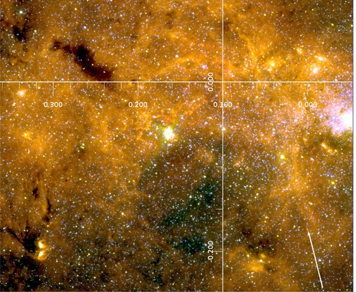
Colour composite Spitzer IRAC image of the GC: red at ∼8 μm, green at ∼5.8 μm, blue at ∼3.6 μm. The image size is 24.8 arcmin × 20.5 arcmin corresponding to 60 pc × 50 pc at a distance of 8 kpc. Galactic coordinates are indicated. The arrow at the lower-right corner points to WR 102ka. The length of the arrow is 250 arcsec (≈10 pc). The bright cluster at the right edge of the image is the Central Cluster around Sgr A*.
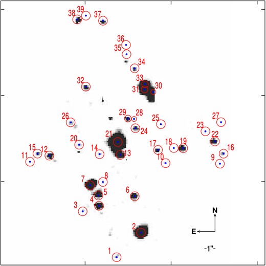
Image of the collapsed grand mosaic cube. Open circles mark the detected sources with their running number in Table 2. The image size is 33.6 arcsec × 38.5 arcsec (1.3 pc × 1.45 pc).
The adaptive optics facility could not be used because there is no sufficiently bright reference star in the neighbourhood. The log of observations is given in Table 1. ABBA (science field – sky – sky – science field) cycles were performed at each pointing. To obtain flux-calibrated spectra, standard stars were observed at similar airmass and in the same mode as the science targets. During our observations, the seeing was between 0.6 and 1.1 arcsec. Thus, the angular resolution of our observations is limited by seeing.
Log of observations.
| Obs. block | Date | RA (J2000) | Dec. (J2000) | Exp. | Skya | Standards | Average |
|---|---|---|---|---|---|---|---|
| (ID) | 2009 | 17h46m | −29°01′ | time (s) | HIPb | seeing (arcsec) | |
| 361412 | May 15 | |$18{.\!\!\!\!\!^{{{\rm s}}}}23$| | 21|${^{\prime\prime}_{.}}$|1 | 150 | B1 | 88857 | 0.63 |
| 361414 | May 15 | |$19{.\!\!\!\!\!^{{{\rm s}}}}04$| | 28|${^{\prime\prime}_{.}}$|3 | 150 | B2 | 88857 | 1.04 |
| 361416 | May 28 | |$18{.\!\!\!\!\!^{{{\rm s}}}}48$| | 28|${^{\prime\prime}_{.}}$|3 | 150 | B1 | 85223 | 1.10 |
| 361418 | June 29 | |$17{.\!\!\!\!\!^{{{\rm s}}}}94$| | 28|${^{\prime\prime}_{.}}$|7 | 30 | B2 | 88857 | 1.07 |
| 361420 | June 27 | |$18{.\!\!\!\!\!^{{{\rm s}}}}76$| | 37|${^{\prime\prime}_{.}}$|1 | 150 | B1 | 88857 | 1.02 |
| 361422 | June 27 | |$18{.\!\!\!\!\!^{{{\rm s}}}}21$| | 37|${^{\prime\prime}_{.}}$|0 | 10 | B1 | 88201 | 0.91 |
| 361424 | June 27 | |$17{.\!\!\!\!\!^{{{\rm s}}}}67$| | 37|${^{\prime\prime}_{.}}$|1 | 150 | B1 | 88857 | 0.78 |
| 361426 | June 27 | |$17{.\!\!\!\!\!^{{{\rm s}}}}12$| | 37|${^{\prime\prime}_{.}}$|2 | 150 | B2 | 88857 | 0.91 |
| 361428 | June 29 | |$18{.\!\!\!\!\!^{{{\rm s}}}}39$| | 44|${^{\prime\prime}_{.}}$|2 | 150 | B1 | 88201 | 0.97 |
| 361430 | June 29 | |$17{.\!\!\!\!\!^{{{\rm s}}}}85$| | 44|${^{\prime\prime}_{.}}$|2 | 150 | B2 | 105164 | 0.90 |
| 361432 | June 29 | |$17{.\!\!\!\!\!^{{{\rm s}}}}91$| | 51|${^{\prime\prime}_{.}}$|4 | 150 | B1 | 88857 | 1.04 |
aSky fields B1 and B2 were centred at the coordinates |$17^{\rm h}46^{\rm m}7{.\!\!\!\!\!^{{{\rm s}}}}22$|, −29°02′54|${^{\prime\prime}_{.}}$|4 and |$17^{\rm h}46^{\rm m}29{.\!\!\!\!\!^{{{\rm s}}}}47{\rm }$|, −28°59′14|${^{\prime\prime}_{.}}$|2, respectively.
bHipparcos catalogue names of standard stars.
The raw data were cleaned with the tool lacosmic (van Dokkum 2001) and a self-written tool for removing artefacts and hot pixels. The further reduction of the data was primarily performed with the ESO pipeline tool esorex, version 3.9.6 (Modigliani et al. 2007).
Sky subtraction for the science observations was performed using the standard pipeline. The wavelength calibration was done by using a Ne–Ar lamp.
Each science observation was flux calibrated. Early BV-type stars were observed as calibration sources, because their spectra are relatively featureless in the K band. The model fluxes of these B-type stars were taken from PoWR models (see Section 4). Accidentally, a foreground B-type star (number 38 in Table 2) is present in our science field. The Two Micron All Sky Survey (2MASS) photometry of this star was used to fine-tune our final flux calibration.
Catalogue of the detected stellar sources.
| No. | RA | Dec. | |$K_{\rm s}^a$| | Spectral | Lumin. | Vrad |
|---|---|---|---|---|---|---|
| 17h46m | −29°01′ | (mag) | type | class | (km s−1) | |
| 1 | |$18{.\!\!\!\!\!^{{{\rm s}}}}0981$| | 54|${^{\prime\prime}_{.}}$|8277 | 14.0 | K3 | II | 105 |
| 2 | |$17{.\!\!\!\!\!^{{{\rm s}}}}8638$| | 51|${^{\prime\prime}_{.}}$|2778 | 10.4 | M5-6 | I-II | 30 |
| 3 | |$18{.\!\!\!\!\!^{{{\rm s}}}}4277$| | 48|${^{\prime\prime}_{.}}$|1673 | 14.2 | K5 | II | 15 |
| 4 | |$18{.\!\!\!\!\!^{{{\rm s}}}}2739$| | 47|${^{\prime\prime}_{.}}$|3639 | 12.3 | M3 | I-II | −25 |
| 5 | |$18{.\!\!\!\!\!^{{{\rm s}}}}2739$| | 45|${^{\prime\prime}_{.}}$|8601 | 12.8 | M2 | I | 130 |
| 6 | |$17{.\!\!\!\!\!^{{{\rm s}}}}9224$| | 45|${^{\prime\prime}_{.}}$|9700 | 12.7 | M1 | I | −100 |
| 7 | |$18{.\!\!\!\!\!^{{{\rm s}}}}3545$| | 44|${^{\prime\prime}_{.}}$|3839 | 11.2 | M4 | I | 225 |
| 8 | |$18{.\!\!\!\!\!^{{{\rm s}}}}2300$| | 43|${^{\prime\prime}_{.}}$|9032 | 14.0 | K1 | I-II | 40 |
| 9 | |$17{.\!\!\!\!\!^{{{\rm s}}}}1021$| | 41|${^{\prime\prime}_{.}}$|2459 | 14.5 | K2 | II | 275 |
| 10 | |$17{.\!\!\!\!\!^{{{\rm s}}}}6221$| | 41|${^{\prime\prime}_{.}}$|1566 | 14.3 | M0 | II-III | 15 |
| 11 | |$18{.\!\!\!\!\!^{{{\rm s}}}}9478$| | 41|${^{\prime\prime}_{.}}$|0399 | 15.8 | lateb | ||
| 12 | |$18{.\!\!\!\!\!^{{{\rm s}}}}7500$| | 40|${^{\prime\prime}_{.}}$|0786 | 13.3 | K5 | I-II | 35 |
| 13 | |$18{.\!\!\!\!\!^{{{\rm s}}}}0615$| | 39|${^{\prime\prime}_{.}}$|9550 | 12.2 | M1 | I | −10 |
| 14 | |$18{.\!\!\!\!\!^{{{\rm s}}}}2666$| | 39|${^{\prime\prime}_{.}}$|8657 | 14.1 | K0 | I-II | 100 |
| 15 | |$18{.\!\!\!\!\!^{{{\rm s}}}}8672$| | 39|${^{\prime\prime}_{.}}$|7833 | 13.8 | M0 | II | 260 |
| 16 | |$17{.\!\!\!\!\!^{{{\rm s}}}}0654$| | 39|${^{\prime\prime}_{.}}$|7902 | 13.9 | M1 | II | 50 |
| 17 | |$17{.\!\!\!\!\!^{{{\rm s}}}}6953$| | 39|${^{\prime\prime}_{.}}$|2477 | 13.5 | M2 | II | −100 |
| 18 | |$17{.\!\!\!\!\!^{{{\rm s}}}}5488$| | 38|${^{\prime\prime}_{.}}$|9731 | 14.8 | K2 | II-III | 135 |
| 19 | |$17{.\!\!\!\!\!^{{{\rm s}}}}4536$| | 39|${^{\prime\prime}_{.}}$|0005 | 12.5 | K3 | I | 55 |
| 20 | |$18{.\!\!\!\!\!^{{{\rm s}}}}4644$| | 38|${^{\prime\prime}_{.}}$|4856 | 14.0 | K3 | I-II | 135 |
| 21 | |$18{.\!\!\!\!\!^{{{\rm s}}}}0908$| | 38|${^{\prime\prime}_{.}}$|0942 | 8.7 | WN9-10 | 60 | |
| 22 | |$17{.\!\!\!\!\!^{{{\rm s}}}}1460$| | 38|${^{\prime\prime}_{.}}$|0118 | 12.8 | M2 | I | −75 |
| 23 | |$17{.\!\!\!\!\!^{{{\rm s}}}}2412$| | 36|${^{\prime\prime}_{.}}$|5424 | 14.3 | K2 | II | 40 |
| 24 | |$17{.\!\!\!\!\!^{{{\rm s}}}}9150$| | 36|${^{\prime\prime}_{.}}$|0892 | 13.1 | M1 | I-II | 65 |
| 25 | |$17{.\!\!\!\!\!^{{{\rm s}}}}6733$| | 35|${^{\prime\prime}_{.}}$|5055 | 14.6 | K3 | II | 170 |
| 26 | |$18{.\!\!\!\!\!^{{{\rm s}}}}5449$| | 35|${^{\prime\prime}_{.}}$|2377 | 13.8 | K0 | I | 20 |
| 27 | |$17{.\!\!\!\!\!^{{{\rm s}}}}0874$| | 35|${^{\prime\prime}_{.}}$|2583 | 14.6 | lateb | ||
| 28 | |$17{.\!\!\!\!\!^{{{\rm s}}}}9297$| | 34|${^{\prime\prime}_{.}}$|7502 | 14.2 | K4 | II | −5 |
| 29 | |$17{.\!\!\!\!\!^{{{\rm s}}}}9883$| | 34|${^{\prime\prime}_{.}}$|6953 | 13.2 | M0 | I-II | −5 |
| 30 | |$17{.\!\!\!\!\!^{{{\rm s}}}}7466$| | 30|${^{\prime\prime}_{.}}$|8295 | 11.3 | M4 | I | 130 |
| 31 | |$17{.\!\!\!\!\!^{{{\rm s}}}}8271$| | 30|${^{\prime\prime}_{.}}$|4587 | 12.1 | M1 | I | 130 |
| 32 | |$18{.\!\!\!\!\!^{{{\rm s}}}}3984$| | 30|${^{\prime\prime}_{.}}$|0604 | 13.4 | M2 | II | 0 |
| 33 | |$17{.\!\!\!\!\!^{{{\rm s}}}}8271$| | 29|${^{\prime\prime}_{.}}$|7102 | 11.3 | M4 | I-II | 130 |
| 34 | |$17{.\!\!\!\!\!^{{{\rm s}}}}9224$| | 27|${^{\prime\prime}_{.}}$|3962 | 13.6 | K4 | I-II | 160 |
| 35 | |$18{.\!\!\!\!\!^{{{\rm s}}}}0029$| | 25|${^{\prime\prime}_{.}}$|3500 | 14.9 | K4 | II-III | 65 |
| 36 | |$18{.\!\!\!\!\!^{{{\rm s}}}}0103$| | 23|${^{\prime\prime}_{.}}$|9973 | 14.8 | K2 | III | −105 |
| 37 | |$18{.\!\!\!\!\!^{{{\rm s}}}}2300$| | 20|${^{\prime\prime}_{.}}$|4749 | 12.9 | K3 | I | −30 |
| 38 | |$18{.\!\!\!\!\!^{{{\rm s}}}}4790$| | 20|${^{\prime\prime}_{.}}$|2963 | 12.0 | B3-5 | IV-V | 0 |
| 39 | |$18{.\!\!\!\!\!^{{{\rm s}}}}3984$| | 19|${^{\prime\prime}_{.}}$|7470 | 14.8 | M0 | III | 150 |
aMagnitudes derived from our flux-calibrated spectra, using the 2MASS filter transmission function (Skrutskie et al. 2006).
bToo faint for closer classification.
The flux-calibrated 3D data cubes of the individual fields were combined to a grand mosaic cube. This cube was ‘collapsed’, i.e. summed over all wavelengths for the purpose of point source detection. The point spread function (PSF) was obtained from our observations of standard stars and applied for the source detection in the science fields. We securely detect 39 point sources in the observed field (see Table 2 and Fig. 2).
Our observations are sensitive down to an apparent magnitude of Ks = 14.8 mag. With the reddening towards WR 102ka (Barniske et al. 2008), the extinction in the K band amounts to about 3 mag. Thus, at the distance of 8 kpc, our observations are sensitive to absolute K-band magnitudes <−2.8 mag.
We considered the possibility that stars fainter than WR 102ka in the K band and located within ∼ 1 arcsec from WR 102ka may remain undetected. Especially, hotter objects would not be easily distinguishable from imaging and photometry alone. Fortunately, we can use the combination of imaging, photometry and line spectrum. We estimate that a contribution of 10 per cent from OB stars to the K-band spectrum of WR 102ka would not escape from our detection because of their He- and Brγ-line features. How many OB stars can be hidden below this limit? The sensitivity of our observations (K = 14.8 mag) is 6 mag (∼250 times) fainter than WR 102ka (K = 8.7, see Table 2) and corresponds to a main-sequence star of about 15 M⊙ (based on the evolutionary tracks by Brott et al. 2011). Thus, about 25 such B-type stars could be hidden within the PSF of WR 102ka. However, more massive stars would be easier to detect. Consider, for instance, an O star of 40 M⊙ and Teff = 30 kK. Such star would have an absolute K magnitude of −5.1 mag, which is 3.7 mag or a factor of 20 fainter than WR 102ka. Thus, a maximum of two such 40 M⊙ stars could be outshined by WR 102ka.
3 CATALOGUE, SPECTRAL CLASSIFICATION AND RADIAL VELOCITIES MEASUREMENTS
The flux-calibrated spectra of all stars were extracted from the data cubes, and their spectral types were determined. With two exceptions, all stars have stellar spectra of late types. A closer classification was obtained from the CO absorption bands, specifically 12CO and 13CO, adopting standard criteria (Goorvitch 1994; Liermann et al. 2009).
We detect only two early-type stars in the field: WR 102ka and a star of spectral type B3-5 (No. 38 in Table 2). The catalogue search revealed that the latter star is an optical source (SPMID 5080099266) of V = 13.77 mag (Girard et al. 2011). We complemented its K-band spectrum obtained with SINFONI with available photometric measurements. These data were fitted with a PoWR model spectrum, and stellar parameters were, thus, obtained (Fig. 3). The star has much lower reddening than the GC region, and is therefore undoubtedly a foreground object at a distance of about ∼2.5 kpc. Its effective temperature is Teff ≈ 16 kK.
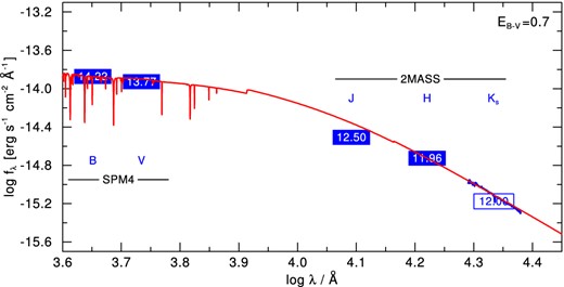
Spectral energy distribution of star No. 38 (alias SPMID 5080099266). The blue boxes indicate the B, V and 2MASS photometric magnitudes. The SINFONI K-band spectrum can be seen as a blue thin line. Overplotted as thick red line is the synthetic spectrum from the PoWR model with Teff = 16 kK and log L/L⊙ = 3.2 for a distance of 2.5 kpc.
Our observations would also be capable to detect massive young stellar objects (MYSOs) if they were present. However, none of the stars in our sample shows spectral features characteristic for MYSOs, such as emissions from CO bands or Brγ (Bik, Kaper & Waters 2006).
The radial velocities of WR 102ka and the other stars were determined from the Doppler shift of prominent stellar lines in their spectra. We estimate that the Doppler shifts are accurate to about 40 km s−1, which corresponds to slightly more than one detector pixel in wavelength.
Radial velocities of late-type stars are determined from the first three band heads of the 12CO λ2.293 μm (2–0), λ2.322 μm (3–1) and λ2.352 μm (4–2) molecular transitions (Gorlova et al. 2006; González-Fernández et al. 2008), where e.g. (2–0) stands for the change in the vibrational quantum number of the molecule from ν = 2 to ν = 0. These three measurements were averaged, and the results are given in Table 2 and Fig. 4. The range of radial velocities of the late-type stars detected in our observed field is similar to that in other nearby areas of the GC region (Liermann et al. 2009).

Radial velocities of the stars in our SINFONI field. The vertical axis gives the source number from Table 2. The shaded area is centred on Vrad(WR 102ka) = 60 km s−1, while its width roughly corresponds to the uncertainty of the measurements.
Stellar wind lines are not symmetric. To determine the radial velocity of WR 102ka, we therefore compared our model to the observation (see Fig. 5 and Section 4). We applied different radial velocity shifts to the model spectrum and calculated the difference to the observation. The χ2 sum has a pronounced minimum for a radial velocity of 60 km s−1. The visual inspection confirms that this value provides a consistent fit for all prominent lines in the spectrum.
![Observed SINFONI spectrum of WR 102ka (blue solid line) together with best-fitting PoWR model spectrum (red dashed line) with luminosity log Lbol[L⊙] = 6.47 ± 0.05, hydrogen abundance X(H) = 30 ± 5 per cent, mass-loss rate $\log {\dot{M}[\mathrm{M}_{\odot }\,{\rm yr}^{-1}]}=-4.6\pm 0.1$, terminal wind speed v∞ = 400 km s−1 and radial velocity 60 km s−1.](https://oup.silverchair-cdn.com/oup/backfile/Content_public/Journal/mnras/436/4/10.1093/mnras/stt1817/2/m_stt1817fig5.jpeg?Expires=1750340335&Signature=G53mVVIvqpwkUppD4~oIkOBeIa4Xrf114RYjLpRmzz9fBiaBw9PbOqSac9EQ~grPHi0xT-dL5YmVpZVTJbx6qCTH3k2GgZccbV1m059KGdcq~VZKf4LHqY7iXgk64FzMbjtpXZYfVRzus5l3dzwyJshThU8WO77pKFdSQvi1iSgFyY8HVLYELskGpboTvT2ObXzznAGD-NwBMHnT0K5Xs6E0ki5rWzQuTtlh2i6WUTFC-8jdWJiJe9mMAw7laRLvNogyER0NqNfTyl9w0yhHxaqf4vz7X19-VmLJUZqqVmp0RaAtC1boTaspt3ppIorbuclSbHFqClwea8QxYJy8DA__&Key-Pair-Id=APKAIE5G5CRDK6RD3PGA)
Observed SINFONI spectrum of WR 102ka (blue solid line) together with best-fitting PoWR model spectrum (red dashed line) with luminosity log Lbol[L⊙] = 6.47 ± 0.05, hydrogen abundance X(H) = 30 ± 5 per cent, mass-loss rate |$\log {\dot{M}[\mathrm{M}_{\odot }\,{\rm yr}^{-1}]}=-4.6\pm 0.1$|, terminal wind speed v∞ = 400 km s−1 and radial velocity 60 km s−1.
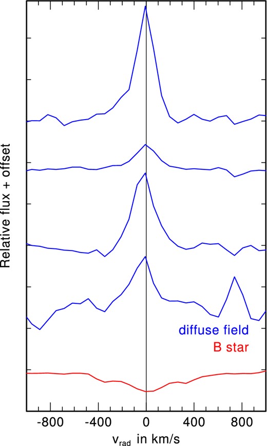
Observed Brγ line in the spectrum of the B-type star No. 38 (red line), compared to the nebular lines at different star-free locations in our field (blue lines), displaced by arbitrary offsets.
Profile shapes might depend on details of the stellar wind model. As a test, we calculated models with different wind velocity laws. The wind model with v∞ = 400 km s−1 and the standard β-velocity exponent β = 1 reproduces the line shapes best. Thus, the wind velocity parameters do not infer a large uncertainty to the radial velocity determination.
We also compared our observed spectrum with that obtained in 2002 by Homeier et al. (2003). No change in radial velocity is detectable between these two observations separated by about seven years.
The radial velocity of the B-type star (No. 38) is obtained from the hydrogen Brγ line, and is found to be 0 km s−1. This is in line with our finding that this star is in the foreground.
There is also diffuse Brγ emission all over our observed field. We selected star-free areas and extracted the nebular spectra. The wavelength of the nebular Brγ emission is unshifted, i.e. the nebular gas has the same radial velocity as the B-type star No. 38 (see Fig. 6). We conclude that this diffuse emission comes from an H ii region that is also located in the foreground, and possibly related to the foreground B-star. According to our model, this star produces log Φ[s−1] = 43.5 hydrogen ionizing photons. Unfortunately, this foreground H ii region contaminates our observations of the circumstellar nebula around WR 102ka.
Our analysis shows that there are no indications for a group of stars comoving with WR 102ka which would have been expected for a star cluster (e.g. Liermann et al. 2009). Thus, we conclude that our observations do not detect a star cluster associated with WR 102ka.
4 SPECTRAL ANALYSIS OF WR 102ka
The earlier spectral analysis of WR 102ka (Barniske et al. 2008) was based on a spectrum obtained in 2002. We found that the star has an unconventionally high luminosity (|$\log {L}[{{\rm L}_{\odot }}]=6.5\pm 0.2$|) at a relatively low stellar temperature (T* = 25.1 kK). The spectral type of WR 102ka was determined as WN10. Barniske et al. (2008) showed that WR 102ka is located above the Humphreys–Davidson limit in the Hertzsprung–Russell diagram (HRD) (see fig. 16 in Barniske et al. 2008). Such stars may be unstable and show large variability changing their location in the HRD on the time-scale of years. In order to investigate whether the stellar parameters of WR 102ka remained stable over more than 7 yr, to check for radial velocity changes (as may be expected in a binary star), and to verify the outstanding stellar parameters derived in the previous work, we obtained and analysed the new spectrum.
As in the previous work, the observed spectrum of WR 102ka was analysed by comparison with Potsdam Wolf-Rayet (PoWR) model atmospheres (Hamann & Gräfener 2004). The PoWR code has been used extensively to analyse the spectra of massive stars in the IR as well in the ultraviolet and optical range (Oskinova, Hamann & Feldmeier 2007; Liermann et al. 2010; Oskinova et al. 2011; Sander, Hamann & Todt 2012). The PoWR code solves the non-LTE radiative transfer in a spherically expanding atmosphere simultaneously with the statistical equilibrium equations and accounts at the same time for energy conservation. Complex model atoms with hundreds of levels and thousands of transitions are taken into account. The computations for this paper include detailed model atoms for hydrogen, helium, carbon, oxygen, nitrogen and silicon. Iron and iron-group elements with millions of lines are included through the concept of superlevels (Gräfener, Koesterke & Hamann 2002). The extensive inclusion of the iron-group elements is important because of their blanketing effect on the atmospheric structure.
Each stellar atmosphere model is defined by its effective temperature, surface gravity, luminosity, mass-loss rate, wind velocity and chemical composition. The gravity determines the density structure of the stellar atmosphere below and close to the sonic point. From the pressure-broadened profiles of photospheric lines, the spectroscopic analysis allows to derive the gravity and thus the stellar mass.
The analysis consists of two coupled steps, the fit of the normalized line spectrum (Fig. 5) and the fit of the spectral energy distribution (Fig. 7). The line fit confirms the parameters obtained in the previous analysis by Barniske et al. (2008): effective temperature T* = 25.1 kK (referring to the radius of Rosseland optical depth 20), hydrogen mass fraction XH = 30 ± 5 per cent, terminal wind velocity v∞ = 400 km s−1, mass-loss rate |$\log {\dot{M}[\mathrm{M}_{\odot }\,{\rm yr}^{-1}]}=-4.7\pm 0.1$| (for a clumping parameter of D = 6).
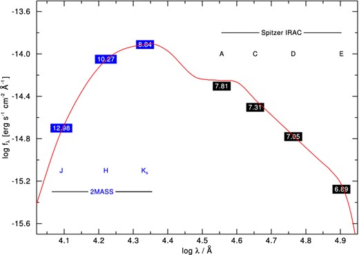
Spectral energy distribution of WR 102ka. The boxes correspond to the photometric magnitudes (as printed in the boxes) measured by 2MASS and Spitzer IRAC. The red line is the continuum from a PoWR model with Teff = 25 kK and log L/L⊙ = 6.47 ± 0.15 at distance modulus and extinction of DM = 14.6 mag and E(B-V) = 8.1 mag, respectively.
When comparing the spectral energy distribution of the model with photometric observations, we tested various extinction curves that are available for the near-IR (Cardelli, Clayton & Mathis 1989; Moneti et al. 2001; Nishiyama et al. 2009). Fortunately, the parameters obtained by the fit [log L, E(B-V)] do not differ significantly. The model shown in Fig. 7 is reddened with the Moneti et al. extinction curve. Finally, we obtain log L/L⊙ = 6.47 ± 0.15, thus confirming the very high stellar luminosity of WR 102ka.
It is known that very luminous massive stars (such as luminous blue variables) display bolometric luminosity variations (e.g. Clark et al. 2009; Sholukhova et al. 2011). The 2MASS measurements employed in Fig. 7 were obtained on 2000 October 7. Our calibrated SINFONI spectrum of WR 102ka obtained in 2009 (see Table 1) gives a slightly higher flux than this 2MASS photometry. The difference corresponds to 0.1 mag and probably just reflects the uncertainty of the calibrations. Nevertheless, it is interesting to note that WR 102ka was reported to vary in the H and J band by 0.16 mag (Matsunaga et al. 2009).
Barniske et al. (2008) speculated that two marginal spectral features which are merely visible in their data might be attributed to N v and He ii, and thus possibly originate from a hotter un-resolved companion. The same weak features seem also to be present in our new spectrum, but the identification remains questionable.
The new data thus verify that the Peony star is one of the most luminous and massive stars known in the Galaxy. According to the latest set of very massive star evolutionary tracks (Yusof et al. 2013), its initial mass was about 150 M⊙, while its current mass amounts to about 100 M⊙ and its age is ∼2 Myr. Using the mass–luminosity relation for very massive stars from Gräfener et al. (2011), the current mass of WR 102ka is ≈110 M⊙.
5 ON THE ORIGIN OF WR 102ka
The hypothesis of optimal IMF sampling implies that a star as massive as WR 102ka was born in a massive star cluster (Weidner et al. 2013). To compare our observations with this hypothesis, we used the mcluster code, which is a publicly available tool for initializing star cluster models and binary-rich stellar populations (Küpper et al. 2011). The simulations predict that ≈300 stars with masses exceeding 20 M⊙ shall be present in a cluster initially containing a star with the mass of WR 102ka. Among these stars ≈10 may be more massive than 100 M⊙. These predictions are in strong disagreement with our observational results.
If WR 102ka would reside in a star cluster with a mass predicted by the simulations, such cluster would be clearly detected in our observations. The characteristic size of a very massive young star cluster is ∼1 pc, while angular resolution of our observations is ≳ 0.024 pc (at the distance of the GC). As can be seen in Fig. 2, WR 102ka is the brightest object in the observational mosaic image. On the detector it covers approximately 10 × 10 pixels. This corresponds to an area with ≈0.1 pc in diameter. Assuming that a hypothetical cluster is ultracompact with a diameter of 0.1 pc, its stellar density would have been >106 M⊙ pc−1. This is an order of magnitude above stellar densities in the most massive clusters in the Local Group (e.g. Portegies Zwart, McMillan & Gieles 2010) and is unrealistic. Also, the spectrum of WR 102ka is well described as originating in a wind of a WR star, with no indications that it is a composite spectrum from many OB and WR stars. We are therefore certain that no massive star cluster is associated with WR 102ka.
We now investigate the possibility that WR 102ka, albeit isolated at present, was formed within a star cluster ∼2 Myr ago. Two scenarios shall be considered: its parental star cluster has dissolved, or WR 102ka was ejected from one of the known (or not yet known) massive star clusters.
The first scenario is relatively easy to dismiss. The self-consistent dynamic N-body star cluster model which accounts for the important tidal field of the Galaxy predicts that the massive clusters in the GC region are not yet dissolved at the age of WR 102ka (Portegies Zwart et al. 2002). An example of an older massive star cluster is the Quintuplet (Liermann et al. 2012).
The ejection scenario may seem more likely. Even a massive star can leave its parental star cluster if it gains sufficiently high spatial velocity either as a result of a supernova explosion in a binary system (Blaauw 1961) or by close stellar encounters during the early dynamical evolution of the cluster (Ambartsumian 1954; Allen, Poveda & Worley 1974; Gies & Bolton 1986). Such stars are commonly termed ‘runaways’.
The radial velocity of WR 102ka is +60 ± 20 km s−1. This is similar to the radial velocities of the atomic and molecular gas at these galactocentric distances that is found to be in the interval between ≳10 km s−1 and ≲+100 km s−1 (Martin et al. 2004; An, Ramírez & Sellgren 2013). However, the radial velocity of WR 102ka is lower than the mean radial velocity of the stars in the Quintuplet cluster, +113 km s−1 (Liermann et al. 2009), or the Arches cluster, +95 km s−1 (Figer et al. 2002).
Mid-IR 24 μm images of the circumstellar nebula around WR 102ka were obtained with the Spitzer telescope.1 Fig. 8 shows the Wide-field Infrared Survey Explorer (WISE) image of this circumstellar dusty nebula (‘Peony nebula’) heated by the stellar radiation of its central star WR 102ka. It was suggested that the nebula contains stellar material that was lost by WR 102ka during previous evolutionary stages (Clark, Larionov & Arkharov 2005; Barniske, Oskinova & Hamann 2008). The central position of the star in its nebula shows that the star basically remained at the same location during its recent evolution.
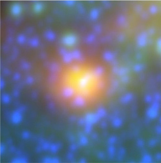
Colour composite WISE image of WR 102ka. Red is at ∼22 μm, green is at ∼12 μm, blue is at ∼3.4 μm. Image size is 3.6 arcmin × 3.6 arcmin. North is up and east is to the left.
Taking the radial velocity as a lower limit to the spatial velocity, WR 102ka travelled at least 130 pc during its lifetime. This is much more than the distance between WR 102ka and the massive star clusters in the GC. Is one of these clusters a possible birthplace for WR 102ka? The Quintuplet and the Central Cluster are older than the age of WR 102ka assuming single star evolution (2 Myr), and therefore it is not likely that the star was formed there. The Arches cluster is younger and might be sufficiently massive for the formation of WR 102ka. However, it seems not likely that just the most massive star has been stripped off from the Arches cluster while many less massive stars remained bound. Summarizing, we conclude that WR 102ka was not formed in any of these clusters.
Stars with supersonic velocities relative to the ambient matter tend to form a bow shock in the direction of its motion (van Buren, Noriega-Crespo & Dgani 1995; Moffat et al. 1998). These bow shocks can be detected with IR imaging (e.g. Kobulnicky, Gilbert & Kiminki 2010). We inspected the IR images of other apparently isolated massive stars in the GC region. Here, we report the apparent presence of bow shocks around two apparently isolated massive stars in the GC region, CXOU J174532.7–285617 (O4-6I)(alias P 114; Dong et al. 2011) and CXOU J144712.2–283121 (WN7-8h; see Fig. 9). Previously, those bow shocks were also noticed by Mauerhan et al. (2010), who reported shell-like or bow-shock like structures around a handful of massive stars in the GC. If the nature of those IR-bright bow shocks is confirmed by future observations, it would indicate that the cluster ejection mechanism operates in the GC region.
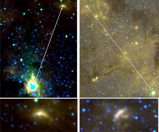
Two bow shocks seen in the colour composite Spitzer IRAC images of the GC region. Red is at ∼8 μm, green is at ∼5.8 μm and blue is at ∼3.6 μm. North is up and east is to the left. Left-hand panels: the arrow (length 4.4 arcmin) points to the bow shock around the O4-6-type supergiant CXOU J174532.7-285617. The bright overexposed object at the bottom is the Central Cluster around Sgr A*. The lower panel zooms on the bow shock. Right-hand panels: the arrow points the bow shock around the WN7-8h star CXOU J144712.2-283121. Its length (22.2 arcmin) indicates its separation from the Quintuplet cluster. The lower panel zooms on the bow shock.
On the other hand, in the IR Spitzer IRAC image of WR 102ka (Fig. 10), no obvious circumstellar structure resembling a bow shock is seen. This presents an additional argument supporting the suggestion that WR 102ka resides at a place of its original formation or not far from it. The majority of isolated massive stars in the GC do not display obvious bow shocks either. On the basis of observational evidence we have today, we shall conclude that the massive star population in the GC region consists of a heterogeneous mixture of stars in clusters, stars which were ejected or stripped from clusters, and stars which were formed outside of clusters. Overall, our results show that at least one very massive star, WR 102ka, is not associated with a star cluster, contrary to the prediction of the IMF optimal sampling hypothesis. The GC region apparently provides an environment where massive stars can form in clusters as well as in relative isolation.
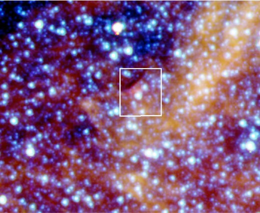
Colour composite Spitzer IRAC image of WR 102ka. Red is at ∼8 μm, green is at ∼5.8 μm and blue is at ∼3.6 μm. The white box illustrates the area covered in our SINFONI observation. Image size is 2.9 arcmin × 3.6 arcmin. North is up and east is to the left.
6 SUMMARY
We obtained the integral field spectroscopic observations of the very luminous and massive WR-type star WR 102ka located in the GC. We confirm previous conclusions that this object is a very massive star with initial mass ≳150 M⊙ and current mass ∼100 M⊙. On the basis of
the absence of early-type stars within ≳1 pc from WR 102ka,
the absence of a group of stars of similar age and comoving with WR 102ka,
the radial velocity of WR 102ka which is similar to the typical galactocentric velocities at this location,
the presence of dusty circumstellar nebula around WR 102ka, which was ejected in previous evolutionary stage of WR 102ka, but containing WR 102ka in its centre,
the absence of a bow shock around WR 102ka, while bow shocks are found around some other massive stars in the GC,
we conclude that one of the most massive and luminous stars in the Galaxy, WR 102ka (Peony nebula star) may have formed in relative isolation.
Based on observations collected at the ESO VLT (programme 383.D-0323(A)). This work has used observations obtained with the Spitzer Space Telescope, which is operated by the Jet Propulsion Laboratory, California Institute of Technology under a contract with National Aeronautics and Space Administration (NASA). This work has extensively used the NASA/IPAC Infrared Science Archive, the NASA's Astrophysics Data System and the SIMBAD data base, operated at CDS, Strasbourg, France. This publication makes use of data products from the 2MASS, which is a joint project of the University of Massachusetts and the Infrared Processing and Analysis Center (IPAC)/California Institute of Technology, funded by the NASA and the National Science Foundation. This publication makes use of data products from the WISE, which is a joint project of the University of California, Los Angeles, and the Jet Propulsion Laboratory/California Institute of Technology, funded by the NASA. We are grateful to the referee for useful comments which helped to improve this paper. Funding for this research has been provided by DLR grant 50 OR 1302 (LMO) and DFG grant HA 1455/22 (AS).
