


Abstract
Most current theoretical models link the launching of relativistic jets from active galactic nuclei to the presence of twisted magnetic fields close to the supermassive black hole. While these models predict a large-scale, ordered, helical magnetic field near the central engine, it is not clear if, and to what extent, this order is preserved further downstream in the jet. Here, we present compelling evidence that suggests that the radio emission from the jet of the quasar 3C 454.3 exhibits multiple signatures of a large-scale, ordered helical magnetic field component at a distance of hundreds of parsecs from the launching point. Our results provide observational support for magnetic jet launching models and indicate that the ordered helical field component may remain stable over a large distance down the jet.
1 INTRODUCTION
Gas accretion on to supermassive black holes (SMBH) is believed to give rise to prominent relativistic jets from active galactic nuclei (Meier, Koide & Uchida 2001). Most current theoretical models relate launching of such powerful outflows to the presence of strongly twisted magnetic fields in the inner part of the accretion disc or the black hole's ergosphere (Blandford & Znajek 1977; McKinney & Blandford 2009). While the jet launching models predict a large-scale, ordered, helical magnetic field close to the central engine, it is not clear if, and to what extent, this order is preserved further downstream in the jet, where instabilities are expected to tangle the field (Meier 2012 and references therein).
The high resolution of very long baseline interferometry (VLBI) experiments are uniquely capable of resolving astrophysical jets down to parsec scales and studying the structure of their magnetic fields. Faraday rotation measure (RM) maps produced by VLBI polarimetry have been used as a diagnostic to probe the jet magnetic field structures (Asada et al. 2002; Gabuzda, Murray & Cronin 2004; Zavala & Taylor 2004; O'Sullivan & Gabuzda 2009; Hovatta et al. 2012, see also Pudritz, Hardcastle & Gabuzda 2012 and references therein), and several apparent gradients and transverse variations indicated that some Faraday screens lie very close to the jet (i.e. the Faraday rotation occurs within the circumjet environment). Faraday rotation occurs when polarized electromagnetic waves propagate through magnetized plasma containing non-relativistic electrons and ions. The resulting rotation of the electric vector position angle (χ) can be described by a linear relation: Δχ = RMλ2, where λ represents the wavelength. The coefficient RM is normally called the Faraday RM and its amount is proportional to the integral of the non-relativistic electron density times the line-of-sight component of the magnetic field. There is a growing body of evidence that the apparent transverse structures in the high angular resolution RM maps of parsec-scale AGN jets may indicate the presence of a large-scale toroidal magnetic field inside the immediate circumjet environment (Asada et al. 2002, 2008a,b; Gabuzda et al. 2004, 2008a; Zavala & Taylor 2004). In contrast, several counter-arguments claim such a magnetic field configuration is inconsistent with the observed low degree of polarization of many sources (e.g. Hughes 2005).
Here, we present compelling evidence that the radio emission from the jet of a quasar exhibits signatures of a large-scale, ordered helical magnetic field component at a distance of hundreds of parsecs from the launching point. The flat-spectrum radio quasar 3C 454.3 (redshift z = 0.859) is one of the brightest and best studied radio-loud quasars (Jorstad et al. 2005). Recently, its intense and highly variable gamma-ray emission has attracted much attention (Vercellone et al. 2008; Striani et al. 2010; Abdo et al. 2011; Bonnoli et al. 2011; Wehrle et al. 2012). Several studies have shown that the radio emission of 3C 454.3 originates in a jet that is oriented very close to our line of sight (viewing angle, φ, ∼1°–3°) with a flow speed of ∼(0.97–0.99) c (where c is the speed of light; Jorstad et al. 2005; Hovatta et al. 2009). High angular resolution radio images obtained by means of VLBI have revealed that at low frequencies 3C 454.3 shows a core–jet morphology, while the inner jet visible at high frequencies appears non-continuous and bent (Pauliny-Toth et al. 1987). Peculiar variations in the structure of the inner jet have also been reported and interpreted as superluminal brightening of the core region (Pauliny-Toth et al. 1987).
A sequence of high angular resolution radio images of 3C 454.3 taken within the last decade shows a strong outburst accompanied by the appearance of a bright superluminal arc-like feature (Britzen et al. 2012), apparently part of the collimated flow which had not been previously visible, thus providing a unique opportunity to study the transverse structure of the jet. Multifrequency polarimetric VLBI imaging of the outflow presented in this paper shows significant transverse asymmetries in intensity, linear polarization and Faraday RM, as is expected in the presence of a large-scale helical magnetic field located within the synchrotron emission region and immediate circumjet environment.
At a redshift of 0.859, each milliarcsecond corresponds to a length of ∼7.7 pc projected on the plane of the sky. Throughout this paper we have adopted a cosmological model with Hubble constant H0 = 71 km s−1 Mpc−1, matter density parameter Ωm = 0.27 and dark energy density ΩΛ = 0.73. In Section 2, we first describe details of our observations and data reduction. Section 3 contains a description of the data analysis and presents the main features of the polarization and Faraday RM maps, including the details of multifrequency image alignment and some implications of the observed structures. Section 4 presents a detailed comparison of our observations with theoretical models of helical magnetic fields. We summarize our results and draw our conclusions in Section 5.
2 OBSERVATIONS AND DATA REDUCTION
All the VLBI data presented in this paper were obtained with the Very Long Baseline Array (VLBA) operated by the National Radio Astronomy Observatory (NRAO). We have used both single-frequency monitoring observations from the MOJAVE (Monitoring Of Jets in Active galactic nuclei with VLBA Experiments) Survey and multifrequency VLBA observations from dedicated experiments.
2.1 15 GHz MOJAVE Survey data
Most of our 15 GHz VLBA maps were either obtained within the MOJAVE Survey or they were retrieved from the NRAO archive and processed by the MOJAVE team (Lister et al. 2009). In addition to the epochs displayed in Fig. 1, observations at 72 epochs between 1995 July 28 and 2011 June 24 are used in the subsequent analysis. Details of the observing setup for each epoch can be found on the MOJAVE web page1 and the data reduction and imaging routines are explained in Lister et al. (2009).
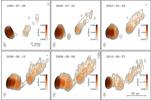
VLBA images of 3C 454.3 at a frequency of 15 GHz (wavelength of 2 cm) from the MOJAVE Survey (Lister et al. 2009). Colours and contours show the total intensity on a logarithmic scale. Only 6 out of 72 analysed epochs are presented here. Observing epochs are indicated at the top left of each image. The sequence of images shows that an arc-like feature developed around the core and started moving outwards with apparent superluminal speed (with its apparent speed increasing from north to the south; Britzen et al. 2012). Synthesized beams are plotted at the bottom-left corner of each image (typical size of ∼0.9 × 0.5 mas).
2.2 Multifrequency VLBA data
In addition to the 15 GHz monitoring, three extra sets of quasi-simultaneous multifrequency VLBI polarimetry data are used in our analysis. On 2005 May 19 we performed VLBA observations of 3C 454.3 at 5.0, 8.3, 15.3, 22.2, 43.1 and 86.2 GHz with observing scans at different frequencies interleaved (Fig. 2). A similar experiment was repeated on 2009 September 22 (without 86 GHz coverage; Fig. 3) as a part of follow-up observations to a γ-ray flare detected by the Fermi-Large Area Telescope (LAT) (Hill 2009). The third multifrequency VLBI data set used in our analysis covers frequencies 8.1, 8.4, 12.1 and 15.4 GHz and was observed as a part of the MOJAVE programme on 2006 March 9. This last data set has been published by Hovatta et al. (2012).
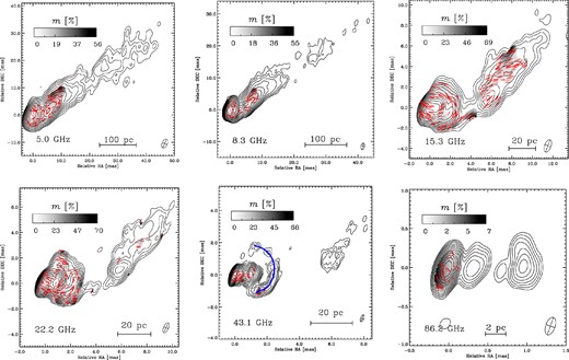
VLBA images of 3C 454.3 at 5.0, 8.3, 15.3, 22.2, 43.1 and 86.2 GHz (top left to bottom right, respectively) observed on 2005 May 19. Contours give the total intensity (logarithmic scale) and colour shows the degree of linear polarization (linear scale). The degree of polarization is only presented where polarized flux is above four times the rms noise level of each map. The synthesized beams used for the maps are presented at the bottom right of each image. Red ticks represent the direction of the apparent (RM-corrected) magnetic field (EVPA+90°, assuming that linear polarization detected in the core region is dominated by optically thin innermost jet components). Position of the arc is marked with a blue curve overplotted on the 43 GHz map.
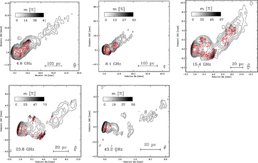
VLBA images of 3C 454.3 at 4.6, 8.1, 15.4, 23.8 and 43.2 GHz (from top left to bottom right, respectively) observed on 2009 September 22. Contours give the total intensity (logarithmic scale) and colour shows the degree of linear polarization (linear scale). The degree of polarization is only presented where polarized flux is above four times the rms noise level of each map. The synthesized beams used for the maps are presented at the bottom right of each image. Red ticks represent the direction of the apparent RM-corrected magnetic field.
The initial calibration of the 2005 May and 2009 September observations was performed in aips using the standard routines for polarimetric VLBI data (see the aips cookbook;2 Leppänen, Zensus & Diamond 1995; Greisen 2003), while the imaging and self-calibration were carried out in the difmap package (Shepherd 1997). The correction terms for instrumental polarization leakage between RCP and LCP signals (the so-called D-terms) were determined by running the aips task LPCAL separately for the target source and each individual calibrator (CTA 102 and 1749+096 in the 2005 May observation, and BL Lac and 2134+004 in the 2009 September observation) and taking the average of the D-term solutions obtained from each source. We kept individual sub-bands (IFs) separated until final imaging step, since D-terms usually vary slightly between the IFs. The polarization purity of the VLBA is high, which results in relatively small D-terms. At C, X and U bands the amplitudes are typically 0.5–3 per cent, except for St Croix that can show values up to 5 per cent. At K and Q bands the D-term amplitudes range from 1 to 8 per cent, with most antennas having values ≲3 per cent. Hancock and St Croix have generally the highest values. At W band (86 GHz), the fitted D-term amplitudes were significantly higher than at other frequencies. While Kitt Peak and Owens Valley showed relatively small amplitudes of 2–4 per cent, North Liberty and Pie Town on the other hand had D-term amplitudes of ∼16 per cent, which start to violate the assumptions of the linearized antenna response model. However, this does not seem to result in any spurious polarization features in the final 86 GHz image (Fig. 2), but it may affect the amount of recovered polarized flux.
The absolute electric vector position angle (EVPA) calibration of the C, X, U, K and Q bands was performed by comparing the integrated VLBI polarization EVPAs of the target and the calibrators to close-in-time observations from the Very Large Array/VLBA polarization calibration data base,3 and single-dish observations from University of Michigan Radio Astronomy Observatory.4 The 86 GHz EVPA at the 2005 May epoch was calibrated by comparing the EVPA of the target source to a polarimetric 3 mm observation carried out at the Institut de RadioAstronomie Millimétrique (IRAM) 30-m telescope 6 d after the VLBA epoch (Wiesemeyer, private communication). Based on the scatter in the EVPA corrections calculated from different sources, the uncertainty in the EVPA calibration is estimated to be 3° in the C, X, U bands, 4° in the K band and 5° in the Q band. In the W band, the EVPA calibration is likely accurate to ∼15° given the non-simultaneity of the VLBA and IRAM 30-m observations and relatively fast variability of the polarization angle at mm-wavelengths.
2.3 Image alignment
Our simultaneous multifrequency coverage allows us to create maps of spectral index, Faraday RM and changes in the degree of polarization across the observed wavelengths. Establishing a relation between the values of each pixel (either flux density or fractional polarization and EVPA) in our maps at different frequencies is only possible after a precise alignment of the images, which were created with the same pixel resolution (0.06 mas for both epochs) and convolved with a common synthesized beam (1.2 × 0.6 and 1.2 × 0.5 mas for 2005 and 2009 epochs, respectively). During the self-calibration step of the VLBA data reduction, the absolute coordinate position of the source is lost. The centroid of the image is not the same for different frequency bands and therefore an extra step is needed to align the images whenever comparison between two or more bands is necessary. This can be done using bright, optically thin components of the jet, whose position should not depend on the observing frequency, either by using the centroid position of model-fitted components at different frequencies or two-dimensional cross-correlation of the images. For calculating the spectral index map, we have used a pixel-based two-dimensional cross-correlation algorithm to look for the best alignment of our multifrequency images based on the correlation of the optically thin parts of the jets at different frequencies. All the derived image shifts were verified by examining the spectral index maps before and after the alignment. In the shifted maps, the spectral index gradient along the jet was typically smoother and any optically thin regions apparently upstream of the core disappeared. Also, spectral indices derived from the fluxes of Gaussian components fit in the (u, v) plane are in good agreement with the values of the spectral index map in the corresponding locations.
The alignment uncertainty in the 2D cross-correlation of any two given maps is difficult to determine. However, based on a large core-shift study of 191 sources from the MOJAVE Survey, Pushkarev et al. (2012) assessed typical random errors in the alignment to be of the order of 1/20 of the beam size. Our alignment uncertainties are likely of the same order – in fact, aligning maps by positions of Gaussian components fit in the (u, v) data and by 2D cross-correlation of the images gave identical results within 1/20 of the beam size. The effects of alignment errors on the RM maps were discussed in detail by Hovatta et al. (2012). Based on their tests, they conclude that even if the image alignment is off by ∼1/6 of the beam size, it does not affect the results from the RM maps significantly, especially when the edge or low signal-to-noise regions are not used to make conclusions about the RM structure.
Finally, we note that whenever we compared maps obtained at different observing bands (e.g. in spectral index measurements), we matched the sampled (u, v) ranges at different frequencies by editing the data and convolved the resulting images with a common restoring beam. This ensured that both images contained emission from similar size scales.
3 ANALYSIS AND RESULTS
3.1 The nature of the arc-like feature in the jet
VLBA observations between 1995 July and 2011 June show the appearance of a peculiar structure in the inner radio core which finally emerged as an arc-like feature (hereafter ‘the arc’), expanding and moving outwards with an apparent superluminal speed (Figs 1 and 2; with its apparent speed increasing from north to the south, see Britzen et al. 2012). The appearance of this arc provides a unique opportunity to study the transverse structure of the jet. The illumination of the northern parts of the inner jet which were not visible in the earlier VLBA images may indicate that the width of the flow is much wider than what is normally visible in a single snapshot observation of limited dynamic range. A stacked image, generated by superimposing all the 2 cm images after aligning their core positions, shows that the inner parts of the jet might actually flow more in the direction of the kpc-scale jet at a position angle of ∼−48° (Pauliny-Toth et al. 1987), instead of ∼−90° (Fig. 4; zero degrees is defined towards north and the position angle decreases clockwise).
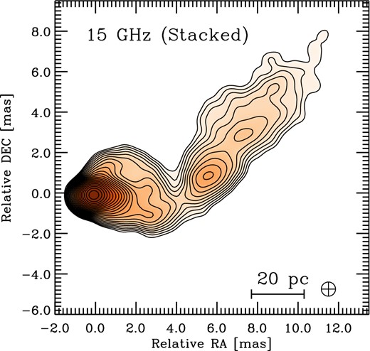
15 GHz stacked image constructed from the superposition of all available VLBA epochs between 1995 and 2011. All the epochs are convolved with the same synthesized beam, shown on the bottom-right corner of the image.
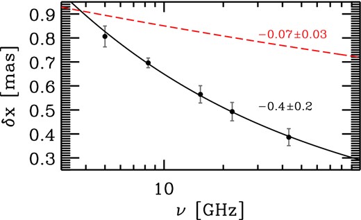
The measured thickness of the arc-like feature (δx) as a function of observing frequency, ν. The thickness at each frequency is estimated as the mean value of the intrinsic (de-convolved) size of the observed radial profile along six different slices across the arc. The solid curve represents the best-fitting solution with δx ∝ ν−0.4 ± 0.2 and the dashed curve shows the maximum expected frequency dependence due to instrumental effects.
Thickness of the arc at different frequency bands. |$\overline{\sigma }$| and |$\overline{\sigma _{\rm beam}}$| are the average FWHM of Gaussian fits to the radial profiles across six different slices and the mean FWHM of the convolution beams projected on the same slices, respectively. Overlapping frequencies of the three pairs of (u, v)-matched images are used to estimate correction factors of ϵ12 = 0.051 mas and ϵ23 = 0.052 mas (where ϵ12 and ϵ23 are calculated from the pairs [CXU,XUK] and [XUK,UKQ], respectively).
| Band | |$\overline{\sigma }$| | |$\overline{\sigma _{\rm beam}}$| |
|---|---|---|
| C (5 GHz) | 1.38 ± 0.06 | 1.12 ± 0.06 |
| X (8 GHz) | 1.06 ± 0.02 | 0.80 ± 0.03 |
| U (15 GHz) | 0.82 ± 0.07 | 0.61 ± 0.03 |
| K (22 GHz) | 0.64 ± 0.11 | 0.40 ± 0.02 |
| Q (43 GHz) | 0.48 ± 0.07 | 0.28 ± 0.01 |
| Band | |$\overline{\sigma }$| | |$\overline{\sigma _{\rm beam}}$| |
|---|---|---|
| C (5 GHz) | 1.38 ± 0.06 | 1.12 ± 0.06 |
| X (8 GHz) | 1.06 ± 0.02 | 0.80 ± 0.03 |
| U (15 GHz) | 0.82 ± 0.07 | 0.61 ± 0.03 |
| K (22 GHz) | 0.64 ± 0.11 | 0.40 ± 0.02 |
| Q (43 GHz) | 0.48 ± 0.07 | 0.28 ± 0.01 |
We find that the arc follows the frequency stratification behaviour expected if the emitting particles are accelerated in a thin layer such as a shock or reconnection region, and such particles are observed as they are advected downstream of the accelerating layer until they radiatively cool via synchrotron radiation. In this scenario, the highest frequency emission mainly arises closest to the shock front, while progressively longer wavelength radiation originates from larger volumes behind the shock (Marscher & Gear 1985). The expected proportionality between the emitting shell's thickness and frequency, δx ∝ ν−1/2, is in agreement with our measured power-law behaviour (decreasing with the index of −0.4 ± 0.2; see Fig. 5).
As mentioned above, in order to correct for the decrease of sensitivity to extended structures towards higher frequencies (caused by differences in (u, v) sampling) when comparing observations made over a broad frequency range, we used piece-wise matched (u, v) coverages in the analysis. To estimate the residual effect that (u, v) sampling differences may have on our measurement of the frequency dependence of the arc's thickness, we carried out simulations. We used the aips task UVMOD to create simulated multifrequency VLBA data at 8, 15, 22 and 43 GHz from the 8 GHz clean model of 3C 454.3. This data set had the same (u, v) sampling and noise properties at different frequency bands as our real observations, but the true sky brightness distribution was exactly the same across all the frequencies. We then piece-wise matched the (u, v) coverages, imaged the data and performed the thickness measurements as with the real data. The resulting thickness values had a very weak frequency dependence as shown by the best-fitting power-law curve in Fig. 5 (red dashed curve). This demonstrates that the observed frequency-dependent thickness of the arc feature is not due to instrumental effects. Therefore, we conclude that the superluminally moving arc-like feature most likely arises from a shock wave resulting from a sudden release of energy at the base of the jet, or a thin reconnection layer where magnetic energy is dissipated.
3.2 Faraday RM and depolarization
Spatial distributions of the degree and angle of linear polarization reveal interesting features (Figs 2 and 3). While the southern part of the arc structure shows a significantly larger degree of polarization, the apparent magnetic vector position angle also swings by more than 90° in the transverse direction. The apparent magnetic field lines seem to follow the contours of the enhanced emission along the arc, which would seem to support the idea that some kind of compression is responsible for creation of the arc and caused the high degree of polarization by compressing a random magnetic field (Laing 1980, see, however, Section 4.2). The same features remain persistent in the images which are observed approximately four years apart.
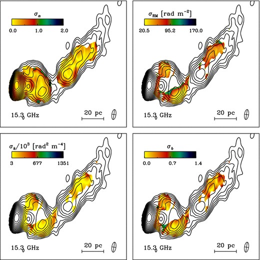
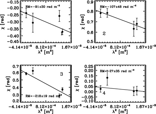
Taking advantage of our simultaneous multifrequency coverage we have, after aligning the images as described in Section 2.3, created maps of spectral index, Faraday RM and depolarization. Spectral index (α, following the nomenclature of Fν ∝ να) maps are constructed from the linear least-squares fit for flux density, Fν, of each pixel versus the observing frequency, ν, in the X, U and K bands. RM maps are derived by performing a linear least-squares fit of the EVPA versus λ2 in each pixel independently. The goodness of fits were estimated by a χ2 criterion. RM maps for 2005 May 19 (Fig. 6) are constructed from images at three different frequencies (8.3, 15.3 and 22.2 GHz maps), while RM maps of 2009 September 22 (Fig. 7) includes four frequencies (8.1, 8.4, 15.4 and 23.8 GHz). For these two epochs, we have used the pacerman5 algorithm (Dolag, Vogt & Enßlin 2005). The pacerman algorithm estimates the possible nπ ambiguities in the direction of the observed electric vector for the regions with high signal-to-noise ratio and uses this information to solve them in the nearby fainter areas. We have introduced a quality cut-off for the RM maps presented in Figs 6 and 7, including only pixels that their polarized flux had higher values than four times of the average rms noise of the same map. We have also implemented an extra safeguard, taking into account only pixels where the direction of the observed E-vector could be determined with an accuracy better than 10°. The 1σ uncertainties in the values of RM (estimated from the uncertainty of the linear fits) are presented in Figs 8 and 9.
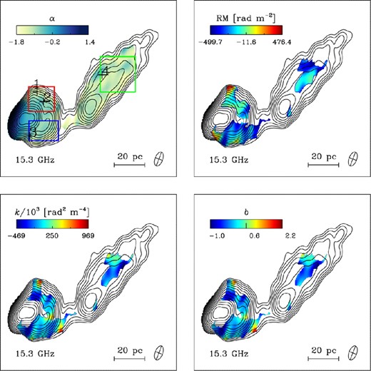
15.3 GHz contour maps of total intensity (logarithmic scale) superimposed with spectral index (α), Faraday RM, Burn law k and power-law index b (m ∝ λb) (from top left to bottom right, respectively) for 2005 May 19 observations. The red, blue and green rectangles indicate the regions for the histograms of Fig. 12. Crosses mark the pixels for which example least-squares fits are shown in Fig. 11 (see also Appendix A). The synthesized beams are plotted at the bottom-left corner of each image.
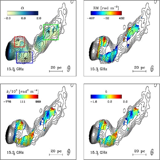
Same as Fig. 6 for 2009 September 22 observations.
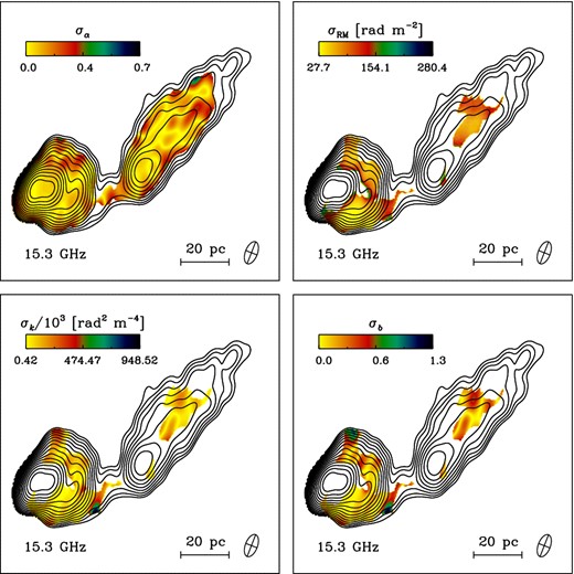
1σ error values corresponding to the maps presented in Fig. 6, estimated from the uncertainty of the least-χ2 fits.
Same as Fig. 8 for 2009 September 22 observations.
Fig. 10 shows an RM map of 3C 454.3, based on observations performed on 2006 March 9 (Hovatta et al. 2012). The derived RM values are based on a least-squares analysis performed by the authors, comparing the observed polarized EVPAs between 8.1, 8.4. 12.1 and 15.4 GHz. Details of their analysis are described in Hovatta et al. (2012). Considering the rather short time gap between our 2005 observations and this RM map (with different resolution but higher signal-to-noise ratio in polarized flux), we found very good agreement between the RM estimates at these epochs. The galactic RM value of −33.5 rad m−2 (Taylor, Stil & Sunstrum 2009) was subtracted from all the observed values.
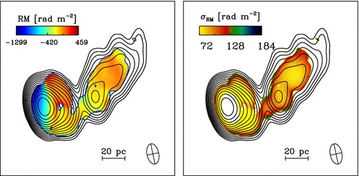
Faraday rotation map of 3C 454.3 based on quasi-simultaneous observations at 8.1, 8.4, 12.12 and 15.37 GHz performed on 2006 March 9 (left) and its corresponding 1σ uncertainties for each pixel (right, see Hovatta et al. 2012 for details).
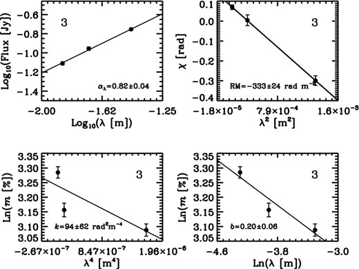
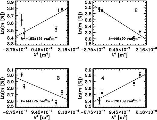
Example plots of flux versus λ, polarization angle versus λ2, logarithm of the degree of polarization versus λ4 and ln (λ) (top left to bottom right, respectively), for the locations marked by the cross labelled with ‘3’ in Fig. 6.
4 DISCUSSION
Observationally, the main challenge in studying the transverse structure of AGN jets is the small width of the visible jet compared to the size of the interferometer beam. This limits the number of independent measurement points one can achieve across the jet width (Taylor & Zavala 2010). One must also keep in mind that close to the edges of the jet the signal to noise ratio drops and random noise can produce artefacts which mimic real physical effects (Hovatta et al. 2012). In our observations, the emergence of a wide arc-like feature illuminated a larger jet width and made it possible to resolve transverse profiles that show significant asymmetry, seen below in Figs 12 –14.
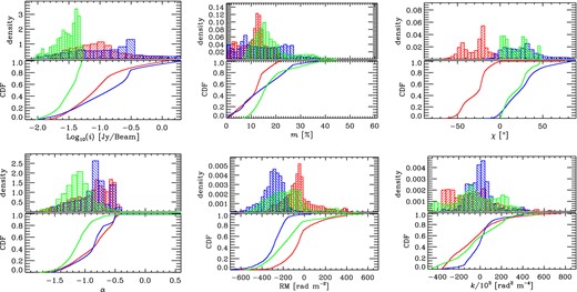
Histograms of logarithm of flux density, percentage of linear polarization, E-vector position angle, spectral index, Faraday RM and Burn law depolarization index (top left to bottom right, respectively) for the pixels in the regions depicted by rectangles in Fig. 6 (red, blue and green colours are corresponding to the boxes with similar colours). The bottom of each panel shows the corresponding cumulative distribution functions (CDF) for each region. Clear gradients in RM, intensity, degree and angle of polarization are visible between pixels located at north (red) and south (blue) of the jet. Northern parts of the jet exhibit a significant increase in the number of pixels which show increasing fractional polarization with wavelength (inverse-depolarization).

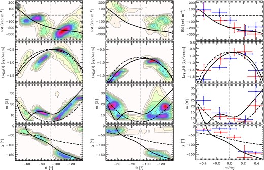
Left: colour scale and contours represent number density distribution of pixels with particular values of Faraday RM, flux density (logarithmic scale), fraction of linear polarization and EVPA as functions of polar angle, Θ (from top to bottom, respectively). Flux density, degree and angle of polarization are derived from the 15.3 GHz maps observed on 2005 May 19. Only pixels with m ≥ 4σm and σχ ≤ 10° were included in generating these profiles. Superimposed on them are profile predictions for a helical magnetic field (solid line) and a shock ordered random field (dashed line) viewed at a small angle, φ ∼ 1° – see body of the text and (Clausen-Brown et al. 2011) for details. Middle: same as left-hand panel but for the 2009 September 22 epoch. Right: transverse profiles along the arc-like feature (from 2005 and 2009 epochs, red and blue colours, respectively). These values are measured using an aperture size 0.8 times that of the synthesized beam. There exist remarkable similarities between the theoretical predictions of the helical field model and our profiles.
The transverse structure most often studied are gradients in RM maps, which are thought to be a sign of helical magnetic fields in parsec-scale jets (Laing 1981; Blandford 1993; Broderick & McKinney 2010). This helical geometry is considered to be a by-product of the toroidal magnetic field in the launching region, which assists in collimating part of the outflow into a narrow shape via magnetic hoop stresses (Chan & Henriksen 1980). Recent analytical and numerical relativistic magnetohydrodynamic (RMHD) studies have shown that a combination of a relativistic outflow and ordered helical magnetic field can produce asymmetries in not just RM profiles, but also in profiles of intensity, fractional linear polarization and spectral index (Clausen-Brown, Lyutikov & Kharb 2011; Porth et al. 2011). The skewness of the profiles is mainly determined by the bulk speed of the flow, viewing angle to the jet and the handedness of the magnetic field. While several unknowns about the details of jet structures make it difficult to use the observed skewed profiles in many AGN jets (Gabuzda et al. 2004; Zavala & Taylor 2004; O'Sullivan & Gabuzda 2009) as robust evidence for the presence of large-scale ordered fields, correlated asymmetrical features in different observables have been proposed as an unambiguous signature of helical magnetic fields (Clausen-Brown et al. 2011). Our observations provide sufficient data to simultaneously measure all of these transverse profiles.
Another sign of the existence of large-scale helical magnetic fields is circular polarization (CP), since the process of Faraday conversion of linear polarization into CP (Jones & Odell 1977) is expected to be particularly effective in a helical magnetic field (Wardle & Homan 2001; Enßlin 2003; Gabuzda et al. 2008b). However, using CP as an indicator for helical fields in 3C 454.3 yields ambiguous results, since this source did not have CP exceeding a 2σ significance level at 5 GHz as reported by Homan, Attridge & Wardle (2001), but was indeed detected later at 15 GHz by Homan & Lister (2006), who found mc = +0.23 ± 0.10 per cent in the core and mc = +0.38 ± 0.10 per cent in the first jet component. Vitrishchak et al. (2008) on the other hand detected mc = −0.29 ± 0.12 per cent at 22 GHz. In any case, we leave an analysis of CP for another work and instead focus here on an analysis of linear polarization and intensity.
4.1 Observed jet transverse structure
Parsec-scale maps of Faraday RM across the jet are shown in Figs 6, 7 and 10. A significant (over 3σ) gradient from north to south along the arc-like feature is seen (at a distance of 1–3 mas from the core), accompanied by a sign reversal of RM. This can be clearly seen in histograms of the RM distribution within the marked regions (Figs 12 and 13) on the northern and southern parts of the jet flow.
Fig. 14 shows the two-dimensional pixel number density contours for the distribution of the RM, flux density, fraction of linear polarization and the direction of the observed E-vector for pixels of Figs 6 and 7 as function of jet polar angle on the plane of the sky, Θ. The jet polar angle is defined by placing the coordinate origin at the inferred location of the SMBH (see Zamaninasab et al., in preparation), where Θ = 0° towards north and increases in the counterclockwise direction. The pixels that contribute to these plots must fulfil two conditions: the pixel's polarized flux for all the observed wavelengths must be greater than four times of the corresponding 1σ errors, and the pixel must be located within a radius of 6 mas from the core.
Our choice of this particular method of plotting is motivated by the assumption that the jet is conical or close to conical in structure, such that all pixels corresponding to some polar angle Θ approximately probe similar regions of local jet cylindrical radius. Thus, in this plotting scheme, Θ is directly analogous to w/wj in the transverse cuts plotted in the right-hand column of Fig. 14, where w is the projected angular coordinate along a transverse cut, and wj is a transverse cut's total angular distance. The advantage of this new plotting scheme is that it avoids the arbitrariness involved in choosing the orientation and location of transverse cuts in the image plane. Thus, our new plotting method provides a much more robust method of determining a jet's transverse structure.
Our two-dimensional contours indeed show clear asymmetries as a function of Θ: RM decreases towards the south (with a sign reversal) and spans approximately 400 rad m−2. Pixels at the southern part of the jet show higher values of intensity and degree of polarization. We have found the most skewed behaviour along the prominent arc feature. While the two-dimensional density contours described above provide a more robust method of determining the jet's transverse structure, we have also chosen transverse cuts in the jet in order to extract profiles for comparison. These profiles are in the right-hand column panels in Fig. 14, and are measured across a transverse slice aligned with the feature.
While it may seem that the presence of such transverse asymmetries are unique to this quasar, it is possible that such features have not been detected before simply due to the limited dynamic range of VLBI imaging. In fact, out of 191 sources in the MOJAVE sample, only 9 show transverse sizes larger than at least two times the synthesized beam in polarized flux, which is needed for detecting asymmetries, and four out of those actually demonstrate significant transverse gradient in RM (Hovatta et al. 2012).
4.2 Helical field model
For a qualitative comparison between our observed jet asymmetries to those expected in helical magnetic field models, we plot the helical magnetic field predictions in Fig. 14. The helical magnetic field model used is a modified version of that used in Clausen-Brown et al. (2011), and has been convolved with a Gaussian beam. The curves do not represent a fit to the data, instead we make straightforward modifications to the model to adapt it to a conical geometry that approximately reproduces the large opening angle 3C 454.3 makes on the sky (see Fig. 15).
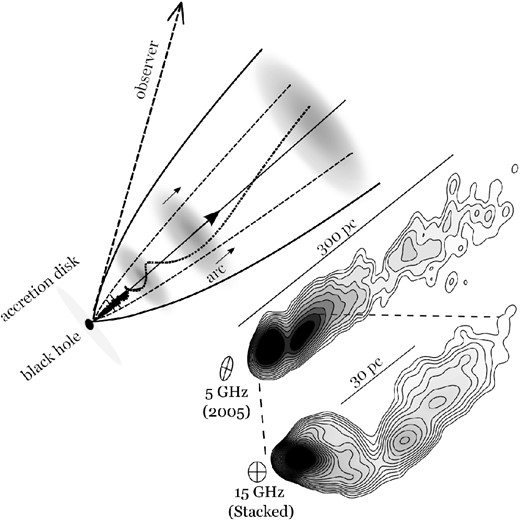
Schematic diagram explaining our helical magnetic field model. The diagram illustrates the geometry of a jet generated from the central black hole surrounded by an accretion disc (not drawn to scale). The magnetic field (dotted line) displays a large-scale ordered right-handed helical structure inside the jet. 5 GHz image of 3C 454.3 observed on 2005 May 19 as well as a 15 GHz stacked image constructed from the superposition of all available VLBA epochs between 1995 and 2011 are presented.
Large-scale helical field models typically overpredict the fractional polarization of jets. On top of the large-scale ordered field, a realistic jet contains a random magnetic field component due to, e.g. accretion disc turbulence (McKinney & Blandford 2009) or jet instabilities. We hypothesize that such a random field component partially depolarizes jet synchrotron emission to reproduce observed values. We model the effect of a random magnetic field component by defining both an average synchrotron emission coefficient originating from a random field component, jrand, and a helical field synchrotron emission coefficient, jhel, such that the total is jtot = jrand + jhel (cf. Wardle et al. 1994; Papageorgiou 2006; Murphy, Cawthorne & Gabuzda 2013). We parametrize jrand such that |$j_{\rm rand}^{\prime }=fK_eB^{\prime 2}$|, where f is a free parameter that determines the strength of the random magnetic field component. Note that |$j_{\rm hel}^{\prime }\propto K_e(B^{\prime }\sin {\tilde{\chi }^{\prime }})^{2}$|, where |$\tilde{\chi }^{\prime }$| is the plasma frame angle between the magnetic field and line of sight. Thus, for f = 0 we recover the results for a pure helical magnetic field, and for f ≫ 1 the jet becomes symmetric and depolarized, as expected for a purely disordered and isotropic magnetic field. We choose an f of 0.45 to reproduce the level of polarization observed while still retaining some jet asymmetry.
Since our model's magnetic field structure remains constant, while the particle density and magnetic field normalization evolve self-similarly with distance from the SMBH (z), the EVPA and polarization behaviour do not change with distance from the SMBH, or z. Thus, the theoretical prediction for polarization and EVPA for a given polar angle (or radial line extending from the SMBH) has only a single value, rather than a range of values. However, our predicted intensity and RM plots do depend on z; thus there are ranges of values they take on for each polar angle. To facilitate the comparison between data and theory, we plot the average values of intensity and RM for each position angle (or radial line).
Fig. 14 shows that 3C 454.3 exhibits the qualitative signature of large-scale magnetic fields predicted by Clausen-Brown et al. (2011): correlated asymmetries. As the real jet is undoubtedly more complex than the simple model we use here, we do not fit the data, other than adjust the random magnetic field component to reproduce the degree of polarization. The model successfully predicted both the high polarization of the jet edges and a correlation in intensity and polarization, where the same side of 3C 454.3 has a higher fractional polarization and intensity. The behaviour of the RM profile also follows our model, though we note the exact location and magnetic field structure of the Faraday rotating screen is highly uncertain.
On a brief theoretical note, we emphasize the importance of the ratio |$B_{{\rm T}}^{\prime }/B_{\rm P}^{\prime }$|, which in our helical field model is of order unity. The qualitative success of our model in explaining 3C 454.3 data corresponding to jet regions at a typical distance of ∼107rg6 (where rg = GM/c2) from the SMBH implies that |$B_{{\rm T}}^{\prime }/B_{\rm P}^{\prime }$| ∼ 1 at large distances from the SMBH. This is surprising in light of jet simulations and magnetic flux freezing arguments which suggest a jet with a Lorentz factor of ∼10 should be toroidally dominated in the rest frame at such large distances measured in rg (e.g. McKinney 2006; Komissarov 2011). However, researchers have suggested that flux freezing is violated such that |$B_{{\rm T}}^{\prime }/B_{\rm P}^{\prime }$| ∼ 1 in AGN jets for both theoretical and observational reasons (Choudhuri & Konigl 1986; Colgate et al. 1998; Lyutikov et al. 2005). Lyutikov et al. (2005), for example, espouse this hypothesis in order to explain several factors: jet EVPA behaviour, the observed low fractional polarizations of jets compared to the theoretically maximum values of ∼0.7, and because magnetohydrodynamical equilibria in which |$B_{\rm T}^{\prime }/B_{\rm P}^{\prime }$| ∼ 1 are more stable against pinch and kink modes. Thus, although controversial, the assumption that |$B_{\rm T}^{\prime }/B_{\rm P}^{\prime }$| ∼ 1 at large distances from the jet launching region is physically plausible assuming some relaxation process drives the magnetic field towards a kink and pinch stable state (which is also the minimum energy state for a force-free plasma, as described in Taylor 1986).
4.3 Alternative theoretical models
As an alternative to the helical field model, we also plot (dashed line, Fig. 14) the predictions for a simple shock model, in which the local shock normal is aligned with the local flow direction in every part of the flow. We use the model developed in Kollgaard, Wardle & Roberts (1990) and Wardle et al. (1994), which depends on the large-scale poloidal field, B0, and a random field component, Br, which is ordered by a shock of compression ratio k. The resulting polarization is determined by the ratio ξ = B0/Br (which we vary with radius so as to produce a dip in the linear polarization at the centre of the jet), as well as the shock compression ratio, k = βdΓd/(βuΓu). As expected, such a model is symmetric, unlike our observations. The prediction for RM from this model is a straight horizontal line since there is no toroidal magnetic field.
Another alternative explanation of these observations could be the existence of an ionized cloud that physically interacts with the jet (Gómez et al. 2000). Assuming an intrinsic spectral index of −0.9 between 15 and 22 GHz, we obtain a lower limit for the free–free opacity at 22 GHz of τff ≥ 0.7 for such a cloud. The free–free opacity is given by |$\tau _{\rm ff}=9.8\times 10^{-3} l\ n_{\rm th}^2\ T^{-1.5}\nu ^{-2}[17.7+\ln {(T^{1.5}\nu ^{-1})}]$|, where l is the column length, nth is the thermal electron density, T is the temperature and ν is the observing frequency (Gómez et al. 2000). Approximating the cloud with a sphere of radius ∼50 pc (sizes larger than this would absorb emission from the northern part of the arc-feature as well), if the cloud has an assumed temperature of ≃104 K, free–free absorption would provide the required opacity for an electron density of |${\simeq } 5\times 10^3 \ \textrm {cm}^{-3}$|. If we combine this with the measured RM of ∼100 ± 50 rad m−2, at the same position, we find the parallel component of its magnetic field to be ∼10−9 G (three orders of magnitude lower than the measured values for galactic clouds of similar density, Troland & Crutcher 2008). Fig. 16 shows the estimates for the parallel component of the magnetic field inside such a cloud as function of its size for three different possible temperature values. The presence of such a cloud south of the jet may explain the apparent bend, but it is unable to reproduce the observed spectral index maps and velocity gradients. Based on these arguments, we consider the presence of a large-scale helical magnetic field as the most likely explanation for the observed skewed profiles. However, it remains to be seen if future RMHD simulations and detailed models of jet–cloud interactions can reproduce such correlated profiles.
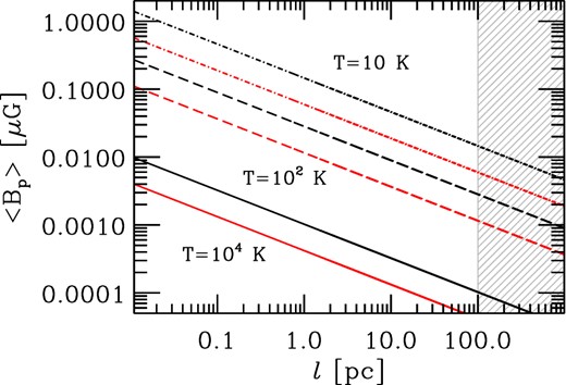
Magnetic field component parallel to the line of sight (Bp) as a function of the cloud size (l) for different values of assumed temperature (103, 102 and 10 K, plotted with solid, dashed and dash–dotted lines, respectively). Black colour represents assumed intrinsic spectral index of αint = −1, while red colour shows the same estimates under assumption αint = −2. Shaded region indicates the size of such interacting cloud that would be too large to match our observations, since it would absorb emission from northern part of the jet as well.
5 CONCLUSIONS
The multiple signatures of large-scale magnetic fields we report here agree with the predictions of MHD jet launching schemes, which require a large-scale poloidal magnetic field at the jet base that develops into a helical magnetic field further downstream in the jet. We propose that the wide arc-like feature that enabled our study of 3C 454.3's transverse structure began as a sudden injection of energy closer to jet base that then propagated down the jet, lighting up the previously unobserved outer regions of jet. The success of our large-scale helical field model in explaining the asymmetries in 3C 454.3's transverse structure implies that the jet frame toroidal magnetic field is similar in strength to the jet frame poloidal field, which is surprising in light of magnetic flux freezing arguments. This hints at non-ideal MHD processes at work in AGN jets such as magnetic relaxation and reconnection.
The existence of a large-scale helical magnetic field at a distance of 107 gravitational radii from the central engine would have profound implications for jet propagation models. It is often assumed that already relatively close to the SMBH (≲102 − 3rg) the jet magnetic field becomes tangled by current driven instabilities, a notion grounded in MHD stability analyses that successfully explain the volatility of Earth-based magnetic fusion experiments (Bateman 1978). Therefore, large-scale helical magnetic fields existing at 107rg from the SMBH indicate that relativistic jets possess some mechanism that stabilizes them against current-driven instabilities. Interestingly, this conclusion has already been hinted at by 3D numerical simulations showing stable jet helical magnetic fields out to 103rg (McKinney & Blandford 2009). Note, however, that our modelling requires a random magnetic field component in addition to the helical field, meaning that some conversion from the ordered to a random field has taken place.
We would like to thank D. Homan, R. Porcas, M. Böck, J.A. Zensus and N. Sabha for their comments on the manuscript. We are grateful to M. Aller and H. Aller for providing data from the University of Michigan Radio Astronomy Observatory monitoring programme. We thank H. Wiesemeyer for providing 3 mm polarization measurements from the IRAM 30-m telescope. This research has made use of data from the MOJAVE data base that is maintained by the MOJAVE team (Lister et al. 2009). The MOJAVE project is supported under NASA Fermi grant 11-Fermi11-0019. This work made use of the VLBA, which is a facility of the National Science Foundation, operated under cooperative agreement by Associated Universities, Inc. This work made use of the Swinburne University of Technology software correlator, developed as part of the Australian Major National Research Facilities Programme and operated under license (Deller et al. 2007). This research has made use of data from the University of Michigan Radio Astronomy Observatory which is supported by the National Science Foundation and by funds from the University of Michigan. Part of this work was done while MZ was supported by the German Deutsche Forschungsgemeinschaft, DFG, via grant SFB 956 project A2. TH was supported by the Jenny and Antti Wihuri foundation. YYK was partly supported by the Russian Foundation for Basic Research (projects 11-02-00368 and 12-02-33101), Research Program OFN-17 of the Division of Physics, Russian Academy of Sciences and by the Dynasty Foundation. ABP was supported by the ‘Non-stationary processes in the Universe’ Program of the Presidium of the Russian Academy of Sciences.
Assuming a 500 pc deprojected distance and an ∼109 M⊙ SMBH.
REFERENCES
APPENDIX A: LINEAR FITS FOR EXAMPLE PIXELS
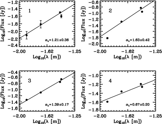
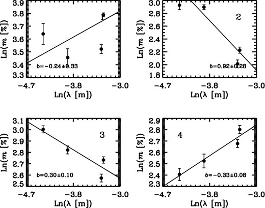
In this appendix, we present example plots of the behaviour of the flux density, EVPA and degree of polarization as functions of λ, λ2, λ4 (and ln [λ]) in order to demonstrate the method used for estimating spectral index, Faraday RM and measures of depolarization (k and b). Each plot corresponds to a pixel marked by a cross with the same number in Figs 6 and 7. These example plots are also indicative of the goodness of the fit for different pixels on our maps (see Figs 8 and 9). The best linear behaviour (as expected) can be seen in relation between flux and observing wavelength (Figs A1 and A5); therefore, we have pretty reliable estimate of the spectral index for each pixel.
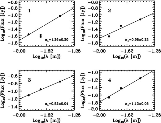
Plots of flux density versus wavelength, λ, for pixels marked in Fig. 6 with the corresponding numbers as depicted in each panel. The best linear fits (solid lines) and estimated slopes, αλ, are also depicted in each image.
While we cannot claim any significant deviation from Δχ ∝ λ2 behaviour over the range of our observing frequencies and within the uncertainties (Figs A2 and A6), there may be hints that whenever fractional polarization increases with increasing wavelength (opposite to the expectation from normal depolarization behaviour due to the Faraday dispersion), deviations from a λ2 relation are more evident (Figs A3 and A7). From the ln (m) − λ4 plots, it is clear that specially for pixels that show inverse-depolarization a λ4 relation may fail to describe the behaviour. This was the main reason to check for a possible power-law relation in ‘m-λ’ space (Figs A4 and A8). However, with our limited number of data points used for each individual fit, it is not possible to distinguish between these different functional forms. The overall behaviour and spatial distribution of the estimated values for both k and b are well in agreement with each other.
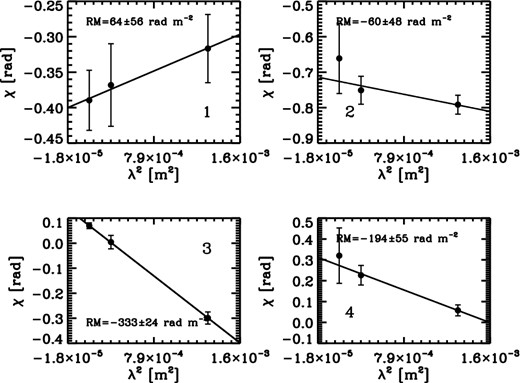
Plots of EVPA, versus λ2 for positions indicated by crosses with the same numbers in Fig. 6. The least chi-squares fit and the estimated Faraday RM are presented for each panel.

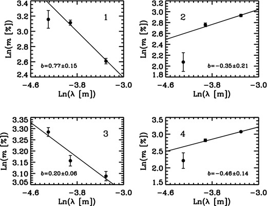
Plots of ln (m) against ln (λ) for the same positions as Figs A1–A3. The best linear fits and the power law indices, b, are presented in each panel.
APPENDIX B: LINK BETWEEN DEPOLARIZATION AND FARADAY RM
In this appendix, we probe the possible global correlation between the values of RM, k and fraction of polarization for the pixels we could have reliable estimate for these values (as shown in Figs 6 and 7). As demonstrated by Burn (1966) and Laing et al. (2008), the wavelength dependence of the fraction of polarization is a function of both the value of RM and its spatial gradient (the so-called differential Faraday rotation and Burn depolarization effects, respectively).
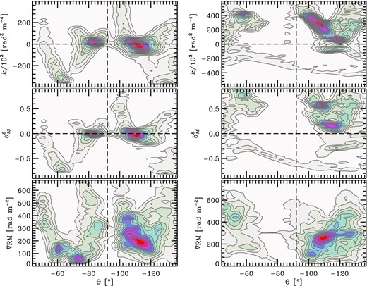
Left: colour scale and contours represent number density of pixels with particular values of Burn's k, de-polarization measure between 8 and 15 GHz, and spatial variations of the Faraday RM as functions of polar angle, Θ, for the 2005 May 19 observations (top to bottom, respectively). Only pixels with m ≥ 4σm and σχ ≤ 10° were included in generating these profiles, similar to the left-hand panel in Fig. 14. Right: same as the left-hand panel but for 2009 September 22 observations (same pixels as Fig. 14 middle panel).
