


Abstract
A major stage of radio interferometric data processing is calibration or the estimation of systematic errors in the data and the correction for such errors. A stochastic error (noise) model is assumed, and in most cases, this underlying model is assumed to be Gaussian. However, outliers in the data due to interference or due to errors in the sky model would have adverse effects on processing based on a Gaussian noise model. Most of the shortcomings of calibration such as the loss in flux or coherence, and the appearance of spurious sources, could be attributed to the deviations of the underlying noise model. In this paper, we propose to improve the robustness of calibration by using a noise model based on Student's t-distribution. Student's t-noise is a special case of Gaussian noise when the variance is unknown. Unlike Gaussian-noise-model-based calibration, traditional least-squares minimization would not directly extend to a case when we have a Student's t-noise model. Therefore, we use a variant of the expectation–maximization algorithm, called the expectation–conditional maximization either algorithm, when we have a Student's t-noise model and use the Levenberg–Marquardt algorithm in the maximization step. We give simulation results to show the robustness of the proposed calibration method as opposed to traditional Gaussian-noise-model-based calibration, especially in preserving the flux of weaker sources that are not included in the calibration model.
1 INTRODUCTION
Radio interferometry gives an enhanced view of the sky, with increased sensitivity and higher resolution. There is a trend towards using phased arrays as the building blocks of radio telescopes (LOFAR1 and SKA2) as opposed to the traditional dish-based interferometers. In order to reach the true potential of such telescopes, calibration is essential. Calibration refers to the estimation of systematic errors introduced by the instrument (such as the beam shape and receiver gain) and also by the propagation path (such as the ionosphere), and correction for such errors, before any imaging is done. Conventionally, calibration is done by observing a known celestial object (called the external calibrator), in addition to the part of the sky being observed. This is improved by self-calibration (Cornwell & Wilkinson 1981), which is essentially using the observed sky itself for the calibration. Therefore, self-calibration entails consideration of both the sky as well as the instrument as unknowns. By iteratively refining the sky and the instrument model, the quality of the calibration is improved by orders of magnitude in comparison to using an external calibrator.
From a signal processing perspective, calibration is essentially the maximum likelihood (ML) estimation of the instrument and sky parameters. An in-depth overview of existing calibration techniques from an estimation perspective can be found in, e.g., Boonstra & van der Veen (2003), van der Veen, Leshem & Boonstra (2004), van der Tol, Jeffs & van der Veen (2007) and Kazemi et al. (2011). All such calibration techniques are based on a Gaussian noise model, and the ML estimate is obtained by minimizing the least-squares cost function using a non-linear optimization technique such as the Levenberg–Marquardt (LM; Levenberg 1944; Marquardt 1963) algorithm. Despite the obvious advantages of self-calibration, there are also some limitations. For instance, Cornwell & Fomalont (1999) give a detailed overview of the practical problems in self-calibration, in particular due to errors in the initial sky model. It is well known that the sources not included in the sky model have lower flux (or loss of coherence), and Martí-Vidal et al. (2010) is a recent study on this topic. Moreover, under certain situations, fake or spurious sources could appear due to calibration as studied by Martí-Vidal & Marcaide (2008).
In this paper, we propose to improve the robustness of calibration by assuming a Student's t-noise model (Gosset 1908) instead of a Gaussian noise model. One of the earliest attempts in deviating from a Gaussian-noise-model-based calibration can be found in Schwab (1982), where instead of minimizing a least-squares cost function, an l1 norm minimization was considered. Minimizing the l1 norm is equivalent to having a noise model which has a Laplacian distribution (Aravkin, Friedlander & van Leeuwen 2012). The motivation for Schwab (1982) to deviate from the Gaussian noise model was the ever present outliers in the radio interferometric data.
In a typical radio interferometric observation, there is a multitude of causes for outliers in the data.
Radio frequency interference caused by man-made radio signals is a persistent cause of outliers in the data. However, data affected by such interference are removed before any calibration is performed by flagging (e.g. Offringa et al. 2010). But there might be faint interference still present in the data, even after flagging.
The initial sky model used in self-calibration is almost always different from the true sky that is observed. Such model errors also create outliers in the data. This is especially significant when we observe a part of the sky that has sources with complicated, extended structure. Moreover, during calibration, only the brightest sources are normally included in the sky model and the weaker sources act together to create outliers.
During day-time observations, the Sun could act as a source of interference, especially during high solar activity. In addition the Galactic plane also affects the signals on short baselines.
An interferometer made of phased arrays will have sidelobes that change with time and frequency. It is possible that a strong celestial source, faraway from the part of the sky being observed, will pass through such a sidelobe. This will also create outliers in the data.
To summarize, model errors of the sky as well as the instrument will create outliers in the data and in some situations calibration based on a Gaussian noise model will fail to perform satisfactorily. In this paper, we consider the specific problem of the effect of unmodelled sources in the sky during calibration. We consider ‘robustness’ to be the preservation of the fluxes of the unmodelled sources. Therefore, our prime focus is to minimize the loss of flux or coherence of unmodelled sources, and our previous work (Yatawatta, Kazemi & Zaroubi 2012) has measured robustness in terms of the quality of calibration.
Robust data modelling using Student's t-distribution has been applied in many diverse areas of research, and Lange, Little & Tylor (1989), Bartkowiak (2007) and Aravkin et al. (2012) are few such examples. However, the traditional least-squares minimization is not directly applicable when we have a non-Gaussian noise model, and we apply the expectation–maximization (EM; Dempster, Laird & Rubin 1977) algorithm to convert calibration into an iteratively reweighted least-squares minimization problem, as proposed by Lange et al. (1989). In fact, we use an extension of the EM algorithm called the expectation–conditional maximization either (ECME) algorithm (Liu & Rubin 1995) to convert calibration to a tractable minimization problem. However, we emphasize that we do not force a non-Gaussian noise model on to the data. In case there are no outliers and the noise is actually Gaussian, our algorithms would work as traditional calibration does.
The rest of the paper is organized as follows. In Section 2, we give an overview of radio interferometric calibration. We consider the effect of unmodelled sources in the sky during calibration in Section 3. Next, in Section 4, we discuss the application of Student's t-noise model in calibration. We also present the weighted LM routine used in calibration. In Section 5, we present simulation results to show the superiority of the proposed calibration approach in minimizing the loss in coherence and present conclusions in Section 6.
Notation. Lowercase bold letters refer to column vectors (e.g. |${\boldsymbol y}$|). Uppercase bold letters refer to matrices (e.g. |${\bf {\sf C}}$|). Unless otherwise stated, all parameters are complex numbers. The matrix inverse, transpose, Hermitian transpose and conjugation are referred to as (.)−1, (.)T, (.)H and (.)⋆, respectively. The matrix Kronecker product is given by ⊗. The statistical expectation operator is given as E{.}. The vectorized representation of a matrix is given by vec(.). The ith diagonal element of matrix |${\bf {\sf A}}$| is given by |${\bf {\sf A}}_{ii}$|. The ith element of a vector |${\boldsymbol y}$| is given by |${\boldsymbol y}_i$|. The identity matrix is given by |${\bf {\sf I}}$|. Estimated parameters are denoted by a hat, |$\widehat{(.)}$|. All logarithms are to the base e, unless stated otherwise. The l2 norm is given by ‖.‖ and the infinity norm is given by ‖.‖∞. A random variable X that has a distribution |$\mathcal {P}$| is denoted by |$X \sim {\mathcal {P}}$|.
2 DATA MODEL
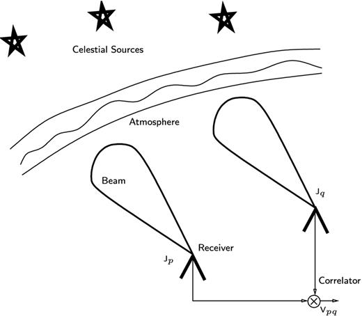
A basic radio interferometer that correlates the signals received from faraway celestial sources. The signals are corrupted by Earth's atmosphere as well as by the receiver beam pattern, and these corruptions are represented by |${\bf {\sf J}}_p$| and |${\bf {\sf J}}_q$|.
3 EFFECT OF UNMODELlED SOURCES IN CALIBRATION
the mean of the effective noise is almost equal to the mean of noise, E{zpq} → E{npq} = 0,
the variance of effective noise is greater than the variance of noise, E{|zpq|2} > E{|npq|2}.
Let us briefly consider the implications of equation (10) above. First, the field of view is |$2\overline{l} \times 2\overline{m}$| in the sky. Now, consider the longest baseline length or the maximum value of |$\sqrt{u^2+v^2}$| to be |$\overline{u}$|. Therefore, the image resolution will be about |$1/\overline{u}$|, and consider the field of view to be of width |$2 \overline{l} \approx P\times 1/\overline{u}$|. In other words, the field of view is P image pixels when the pixel width is |$1/\overline{u}$|. Now, in order for E{zpq} ≈ 0 in equation (10), we need |$|u|>\frac{1}{2 \overline{l}}$| or |$|u|> \overline{u}/P$| (and a similar expression can be derived for |v|). This means that for baselines that are at least 1/P times the maximum baseline length, we can assume E{zpq} ≈ 0.
To illustrate the above discussion, we give a numerical example considering the LOFAR highband array at 150 MHz. The point spread function at this frequency is about 6 arcsec and the field of view is about 10° in diameter. Therefore, P ≈ 10 × 3600/6 = 6000. The longest baselines is about 80 km and for all baselines that are greater than 80/6 = 13 m, the assumptions made above more or less hold.
3.1 SAGE algorithm with unmodelled sources
In our previous work (Kazemi et al. 2011), we have presented the Space Alternating Generalized EM (SAGE; Fessler & Hero 1994) algorithm as an efficient and accurate method to solve equation (7), when the noise model is Gaussian. However, when there are unmodelled sources, as we have seen in this section, the noise model is not necessarily Gaussian.
4 ROBUST CALIBRATION
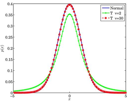
Probability density functions for standard normal distribution and Student's t-distribution, with ν = 2 and 30. At ν = 30, the Student's distribution is indistinguishable from the normal distribution.
Algorithm 1: Robust Levenberg–Marquardt (ECME)
Require: Data |${\boldsymbol y}$|, mapping |${\boldsymbol f}({\boldsymbol \theta })$|, Jacobian |${\bf {\sf J}}({\boldsymbol \theta })$|, ν, initial value |${\boldsymbol \theta }^0$|
1: |${\boldsymbol \theta } \leftarrow {\boldsymbol \theta }^0$|; wi ← 1; λ ← 1
2: whilel < max EM iterations do
3: k ← 0; η ← 2
4: |${\bf {\sf J}}({\boldsymbol \theta }) \leftarrow {\bf {\sf W}} {\bf {\sf J}}({\boldsymbol \theta })$|
5: |${\bf {\sf A}} \leftarrow {\bf {\sf J}}({\boldsymbol \theta })^T{\bf {\sf J}}({\boldsymbol \theta }); {\boldsymbol e}\leftarrow {\bf {\sf W}}({\boldsymbol y}-{\boldsymbol f}({\boldsymbol \theta })); {\boldsymbol g} \leftarrow {\bf {\sf J}}({\boldsymbol \theta })^T {\boldsymbol e}$|
6: found |$\leftarrow (\Vert {\boldsymbol g}\Vert _{\infty } <\epsilon _1); \mu \leftarrow \tau \max {\bf {\sf A}}_{ii}$|
7: while (not found) and (k < max iterations)
8: k ← k + 1; Solve |$({\bf {\sf A}} + \mu {\bf {\sf I}}){\boldsymbol h}={\boldsymbol g}$|
9: if|$\Vert {\boldsymbol h}\Vert <\epsilon _2(\Vert {\boldsymbol \theta }\Vert +\epsilon _2)$|
10: found ← true
11: else
12: |${\boldsymbol \theta }_{new} \leftarrow {\boldsymbol \theta } + {\boldsymbol h}$|
13: |$\rho \leftarrow (\Vert {\boldsymbol e}\Vert ^2 - \Vert {\bf {\sf W}}({\boldsymbol y}-{\boldsymbol f}({\boldsymbol \theta }_{new}))\Vert ^2)/({\boldsymbol h}^T(\mu {\boldsymbol h}+{\boldsymbol g}))$|
14: if ρ > 0 then
15: |${\boldsymbol \theta } \leftarrow {\boldsymbol \theta }_{new}$|
16: |${\bf {\sf J}}({\boldsymbol \theta }) \leftarrow {\bf {\sf W}} {\bf {\sf J}}({\boldsymbol \theta })$|
17: |${\bf {\sf A}} \leftarrow {\bf {\sf J}}({\boldsymbol \theta })^T{\bf {\sf J}}({\boldsymbol \theta }); {\boldsymbol e}\leftarrow {\bf {\sf W}}({\boldsymbol y}-{\boldsymbol f}({\boldsymbol \theta })); {\boldsymbol g} \leftarrow {\bf {\sf J}}({\boldsymbol \theta })^T {\boldsymbol e}$|
18: found |$\leftarrow (\Vert {\boldsymbol g}||_{\infty }\le \epsilon _1)$|
19: μ ← μmax (1/3, 1 − (2ρ − 1)3); η ← 2
20: else
21: μ ← μη; η ← 2η
22: endif
23: endif
24: endwhile
25: Update weights |$w_i\leftarrow \lambda \frac{\nu +1}{\nu + ({\boldsymbol y}_i - {\boldsymbol f}_i({\boldsymbol \theta }))^2}$|
26: Update |$\lambda \leftarrow \frac{1}{N} \sum _{i=1}^N w_i$|
27: Update ν using (24)
28: l ← l + 1
29: endwhile
30: return|${\boldsymbol \theta }$|
5 SIMULATION RESULTS
In this section, we provide results based on simulations to convince the robustness of our proposed calibration approach. We simulate an interferometric array with R = 47 stations, with the longest baseline of about 30 km. We simulate an observation centred at the north celestial pole, with a duration of 6 h at 150 MHz. The integration time for each data sample is kept at 10 s. For the full duration of the observation, there are 2160 data points. Each data point consists of 1081 baselines and 8 real values corresponding to the 2 × 2 complex visibility matrix.
In Fig. 4, we show some of the weak sources (with intensities less than 1 Jy) over a 4° × 4° are of the field of view. In Fig. 5, we have also added the bright sources with slowly varying directional errors. Note that in order to recover Fig. 4 from Fig. 5, directional calibration is essential.
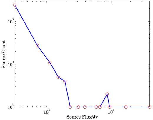
Histogram of the fluxes of the 300 simulated sources. The peak flux is 40 Jy.
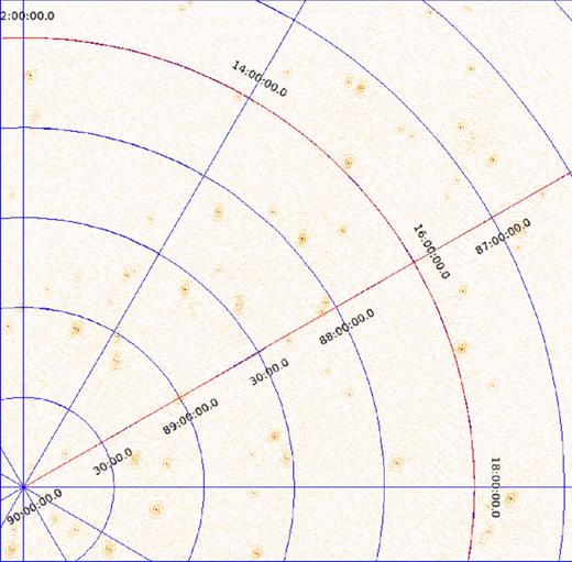
Simulated image of 4° × 4° of the sky, showing only weak sources with intensities less than 1 Jy.

Simulated image of the sky where bright sources with fluxes greater than 1 Jy have been corrupted with directional errors. Due to these errors, there are artefacts throughout the image that make it difficult to study the fainter background sources.
In Fig. 6, we show the image after directional calibration along the bright sources and subtraction of their contribution from the data, using traditional calibration based on a Gaussian noise model. On the other hand, in Fig. 7, we show the image after directional calibration and subtraction using a robust noise model. With respect to the subtraction of the bright sources from the data, both normal calibration and robust calibration show equal performance as seen from Figs 6 and 7.
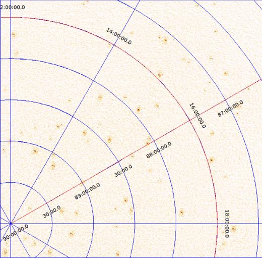
Image of the sky where the bright sources have been calibrated and subtracted from the data to reveal the fainter background sources. The traditional calibration based on a Gaussian noise model is applied.
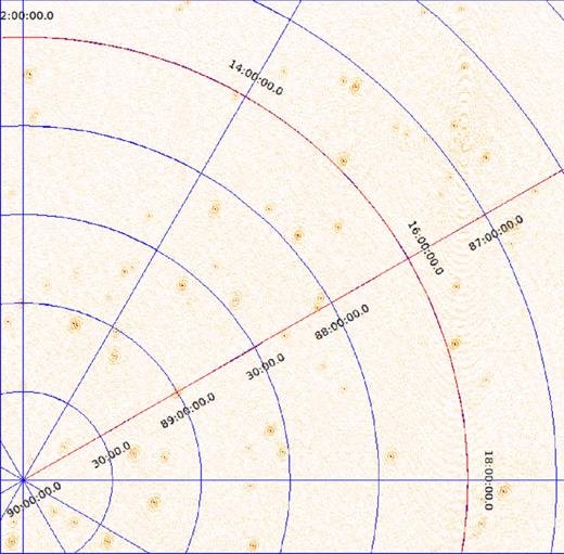
Image of the sky where the bright sources have been calibrated and subtracted from the data to reveal the fainter background sources. The robust calibration proposed in this paper is applied.
We perform Monte Carlo simulations with different directional gain and additive noise realizations for each scenario (i), (ii) and (iii) as outlined previously. For each realization, we image the data after subtraction of the bright sources and compare the flux recovered for the weak sources before and after directional calibration. The directional calibration is performed for every 10 time samples (every 100 s duration). Therefore, the number of data points used for each calibration (N) is 10 × 1081 × 8 = 86 480 and the number of real parameters estimated are 47 × 8 × 28 = 10 528, 47 × 8 × 11 = 4136 and 47 × 8 × 7 = 2632, respectively, for scenarios (i), (ii) and (iii). For each scenario (i), (ii) and (iii), we perform 100 Monte Carlo simulations.
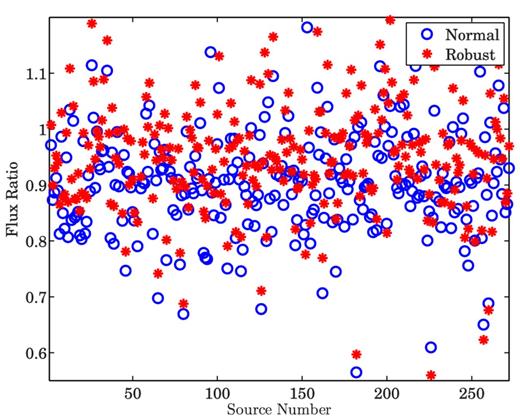
Our performance metric is the ratio between the recovered peak flux of the weak sources and the original flux of each source. We calculate the average ratio (recovered flux/original flux) over all Monte Carlo simulations. In Figs 8– 10, we show the results obtained for scenarios (i), (ii) and (iii), respectively.
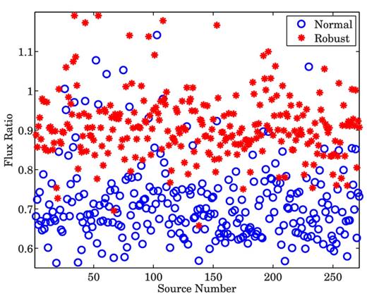
Ratio between the recovered flux and the original flux of each of the weak sources, when bright sources (>1 Jy) are subtracted.
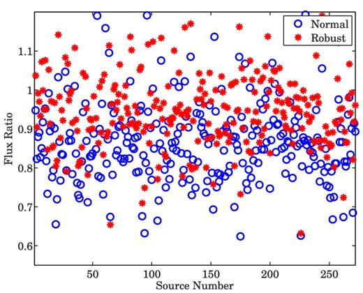
Ratio between the recovered flux and the original flux of each of the weak sources, when bright sources (>2 Jy) are subtracted.
Ratio between the recovered flux and the original flux of each of the weak sources, when bright sources (>5 Jy) are subtracted.
We observe two major characteristics in Figs 8–10. First, we see that as we calibrate over an increasing number of directions (and subtract an increasing number of sources), the recovered flux is reduced. Secondly, in all scenarios, robust calibration recovers more flux compared to normal calibration. To illustrate this point, we also plot in Fig. 11, the ratio between the recovered flux using robust calibration and the recovered flux using normal calibration. As we see from Fig. 11, we almost always get a value greater than 1 for this ratio, indicating that we recover more flux using robust calibration.
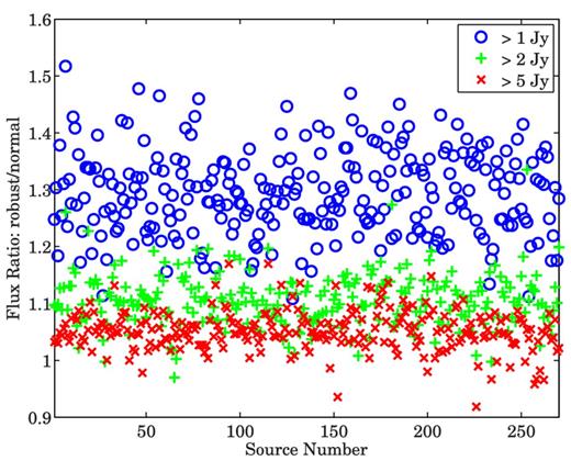
Ratio between the recovered flux using robust calibration and the recovered flux using normal calibration. Almost always, robust calibration recovers more flux compared with normal calibration. The different colours indicate different scenarios where the number of bright sources subtracted is varied.
We summarize our findings in Table 1. We see that at worst case, the performance of normal calibration gives a flux reduction of about 20 per cent compared to robust calibration.
Comparison of the reduction of flux of the weak background sources with normal and robust calibration.
| No. of sources | Lowest flux of the | Average reduction of the flux of weak | |
|---|---|---|---|
| calibrated and | subtracted sources | background sources (per cent) | |
| subtracted | (Jy) | ||
| Normal calibration | Robust calibration | ||
| 28 | 1 | 28.7 | 8.2 |
| 11 | 2 | 12.3 | 3.2 |
| 7 | 5 | 7.9 | 3.1 |
Up to now, we have only considered the sky to consist of only point sources. In reality, there is diffuse structure in the sky. This diffuse structure is seldom incorporated into the sky model during calibration either because it is too faint or because of the complexity of modelling it accurately. We have also done simulations where there is faint diffuse structure in the sky and only the bright foreground sources are calibrated and subtracted. We have chosen scenario (i) in the previous simulation except that we have replaced the sources below 1 Jy with Gaussian sources with peak intensities below 1 Jy and with random shapes and orientations.
In Fig. 12, we have shown the residual image of a 6° × 6° area in the sky after removing all sources brighter than 1 Jy. The residual image is obtained by averaging 100 Monte Carlo simulations. The equivalent image for robust calibration is given in Fig. 13.
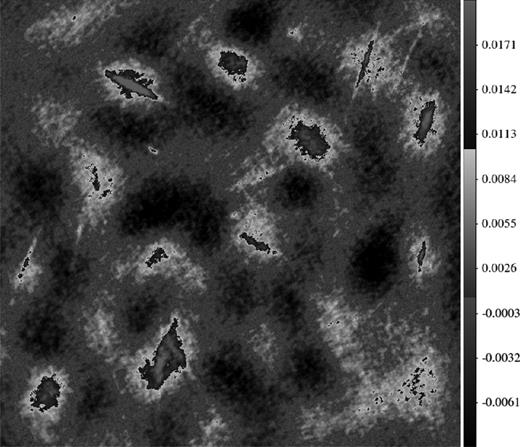
The average residual image of the diffuse structure after subtracting the bright sources by normal calibration. The colour scale is in Jy per PSF.

The average residual image of the diffuse structure after subtracting the bright sources by robust calibration. The colour scale is in Jy per PSF and is the same as in Fig. 12.
As seen from Figs 12 and 13, there is more flux in the diffuse structure after robust calibration. This is clearly seen in the bottom right-hand corner of both figures, where Fig. 13 has more positive flux than in Fig. 12.
6 CONCLUSIONS
We have presented the use of Student's t-distribution in radio interferometric calibration. Compared with traditional calibration that has an underlying Gaussian noise model, robust calibration using Student's t-distribution can handle situations where there are model errors or outliers in the data. Moreover, by automatically selecting the number of degrees of freedom ν during calibration, we have the flexibility of choosing the appropriate distribution even when no outliers are present and the noise is perfectly Gaussian. For the specific case considered in this paper, i.e. the loss of coherency or flux of unmodelled sources, we have given simulation results that show the significantly improved flux preservation with robust calibration. Future work would focus on adopting this for pipeline processing of massive data sets from new and upcoming radio telescopes.
We thank the reviewer, Fred Schwab, for his careful review and insightful comments. We also thank the Editor and Assistant Editor for their comments. We also thank Wim Brouw for commenting on an earlier version of this paper.
The Low Frequency Array.
The Square Kilometre Array.
