


Abstract
The spatial segregation between dwarf spheroidal (dSph) and dwarf irregular galaxies in the Local Group has long been regarded as evidence of an interaction with their host galaxies. In this paper, we assume that ram-pressure stripping is the dominant mechanism that removed gas from the dSphs and we use this to derive a lower bound on the density of the corona of the Milky Way at large distances (R ∼ 50–90 kpc) from the Galactic Centre. At the same time, we derive an upper bound by demanding that the interstellar medium of the dSphs is in pressure equilibrium with the hot corona. We consider two dwarfs (Sextans and Carina) with well-determined orbits and star formation histories. Our approach introduces several novel features: (i) we use the measured star formation histories of the dwarfs to derive the time at which they last lost their gas and (via a modified version of the Kennicutt–Schmidt relation) their internal gas density at that time; (ii) we use a large suite of 2D hydrodynamical simulations to model the gas stripping; and (iii) we include supernova feedback tied to the gas content. Despite having very different orbits and star formation histories, we find results for the two dSphs that are in excellent agreement with one another. We derive an average particle density of the corona of the Milky Way at R = 50–90 kpc in the range ncor = 1.3–3.6 × 10⁻⁴ cm−3. Including additional constraints from X-ray emission limits and pulsar dispersion measurements (that strengthen our upper bound), we derive Galactic coronal density profiles. Extrapolating these to large radii, we estimate the fraction of baryons (missing baryons) that can exist within the virial radius of the Milky Way. For an isothermal corona (Tcor = 1.8 × 10⁶ K), this is small – just 10–20 per cent of the expected missing baryon fraction, assuming a virial mass of 1–2 × 10¹² M⊙. Only a hot (Tcor = 3 × 10⁶ K) and adiabatic corona can contain all of the Galaxy's missing baryons. Models for the Milky Way must explain why its corona is in a hot adiabatic thermal state; or why a large fraction of its baryons lie beyond the virial radius.
1 INTRODUCTION
In the current cosmological framework, the fraction of baryonic matter to dark matter (DM) is known to a high level of precision, thanks to both big bang nucleosynthesis (Pagel 1997) and the study of the cosmic microwave background (e.g. Komatsu et al. 2009; Planck Collaboration et al. 2013). By contrast, the fraction of baryons observed in the form of stars and gas in collapsed structures in the Universe is rather scant, which is commonly referred to as the missing baryon problem. Only massive galaxy clusters appear to have the amount of baryons expected, mostly in the form of hot gas that permeates their deep potential wells (e.g. Sarazin 2009). Galaxy groups and isolated galaxies contain a fraction of detectable baryons which is a factor of ∼10 smaller than the expected fraction and this discrepancy steadily increases with decreasing virial mass (e.g. Read & Trentham 2005; McGaugh et al. 2010).
Disc galaxies represent particularly challenging environments. Applying the cosmological baryon fraction to the virial mass of the Milky Way (MW; 1–2 × 10¹² M⊙; e.g. Wilkinson & Evans 1999), one would predict a total baryonic mass for the Galaxy of ∼2–3 × 10¹¹ M⊙. However, the currently detected mass in stars is ∼5 × 10¹⁰ M⊙ (Dehnen & Binney 1998) while interstellar matter accounts only for <1 × 10¹⁰ M⊙ (Binney & Merrifield 1998; Nakanishi & Sofue 2006). Therefore, ∼70–80 per cent of the MW's baryons are missing. Similar discrepancies are obtained for other disc galaxies of comparable mass (e.g. Read & Trentham 2005).
A commonly accepted solution to this incongruity is that galaxies should be embedded in massive atmospheres – cosmological coronae – of hot gas at temperatures of a few 106 K which contain most of the baryons associated with their potential wells (Fukugita & Peebles 2006). To date, the detection of these coronae has proven rather elusive since at this temperature and density (and assuming a low metallicity) the gas is unable to efficiently absorb or emit photons through metal lines or bremsstrahlung radiation (e.g. Sutherland & Dopita 1993). Some disc galaxies do show X-ray emission outside of their discs, but in most cases this is clearly associated with star formation and the presence of galactic winds (Strickland et al. 2004). In general, owing to contamination from the disc, an unambiguous detection of a cosmological corona is difficult in disc galaxies, unless hot gas is seen at large distances (≳10 kpc) above or below the disc plane. A notable case is the massive galaxy NGC 5746 (Pedersen et al. 2006), where an early claim of an extended X-ray emitting corona was later attributed to an error in the background subtraction in the Chandra data (Rasmussen et al. 2009). This case alone demonstrates that these studies are at the limit of the capabilities of current X-ray facilities (Bregman 2007, but see also Hodges-Kluck & Bregman 2013; Li & Wang 2013).
In the MW, there are several indirect indications of the presence of a hot corona. The first evidence was pointed out by Spitzer soon after the discovery of clouds at high latitudes as a medium capable of providing their pressure confinement (Spitzer 1956). Head–tail shapes of high-velocity clouds (HVCs) are also considered as evidence of an interaction between them and the corona (Putman, Saul & Mets 2011). Unfortunately, all measured distances of HVCs are within 10 kpc from the plane of the disc (e.g. Wakker et al. 2008). Thus, it is not clear whether they are probing the cosmological corona or simply extra-planar hot gas. A perhaps more relevant observation is the asymmetry between the leading and trailing arms of the Magellanic Stream (e.g. Putman et al. 2003), which is seen further out (∼50 kpc) and could result from ram-pressure stripping (see Guhathakurta & Reitzel 1998; Mastropietro et al. 2005; Diaz & Bekki 2012). Finally, X-ray spectra towards bright active galactic nuclei (AGN) show absorption features – in particular O VII, Ne IX and O VIII – characteristic of a corona at T ≳ 106 K. However, the poor velocity resolution of these spectra does not allow us to determine the extent of this medium and the current estimates range from a few kpc to ∼1 Mpc (Nicastro et al. 2002; Bregman & Lloyd-Davies 2007; Yao et al. 2008).
Anderson & Bregman (2010, hereafter AB10) list a number of known indirect pieces of evidence for the Galactic corona. They attempt to use them to give limits on the amount of gas it can contain. For an isothermal corona, they argued that the gas mass should be relatively small – of the order of 10 per cent of the total mass of missing baryons – assuming a Navarro, Frenk & White (1997) (NFW) profile. The fraction can become significantly larger, however, for adiabatic coronae (see also Binney, Nipoti & Fraternali 2009; Fang, Bullock & Boylan-Kolchin 2013). The same authors presented also a possible detection of a corona of missing baryons around the massive spiral NGC 1961 (Anderson & Bregman 2011). Their estimate of the total mass for an isothermal corona is again ∼10 per cent of the baryons that should be associated with the potential well of this galaxy. This estimate comes from an extrapolation as the visible corona extends only to about ∼50 kpc from the centre. Potential problems with this detection come from the fact that this galaxy may be the result of a recent collision (Combes et al. 2009) and shows a rather disturbed H i disc that extends to a distance of 50 kpc from the centre (Haan et al. 2008). A new and more compelling detection is that of the supermassive disc galaxy UGC 12591, where the amount of gas in the corona is estimated to be between 10 (isothermal) and 35 per cent (adiabatic; Dai et al. 2012).
Following Shull, Smith & Danforth (2012), the low-redshift baryon content can be divided as follows: 1.7 per cent in cold gas (H i and He i), 4 per cent in the intracluster medium, 5 per cent in the circumgalactic medium,1 7 per cent in galaxies [stars and interstellar medium (ISM)], 30 per cent in the intergalactic warm–hot ionized medium (WHIM) and 30 per cent in the Lyα forest. This leaves 29 ± 13 per cent of the baryons still missing. From their high-resolution cosmological simulations, these authors found that about half of these missing baryons may be in a hot (T > 106 K) intergalactic WHIM phase.
In this paper, we derive the density of the corona of the MW at large distances (∼50–90 kpc) from the centre using the population of surrounding dwarf spheroidal (dSph) satellites as a probe of the hot halo gas. dSphs are gas-free dwarf galaxies – at least down to current detection limits (e.g. Mateo 1998). They are typically located close to their host galaxy in contrast to the gas-rich dwarf irregulars (dIrrs) that lie at larger distances (Mateo 1998; Geha et al. 2006). The proximity to our Galaxy is believed to be the reason for the removal of material from the dSphs, as several other physical properties are very similar between the two types (e.g. Kormendy 1985; Tolstoy, Hill & Tosi 2009). A similar distance–morphology relation is also observed in dwarf galaxies in other groups (e.g. Geha et al. 2006), suggesting that in addition to supernova (SN) feedback, environmental effects like ram-pressure stripping from a hot corona (Gunn & Gott 1972; Nulsen 1982) or tidal stripping (e.g. Read et al. 2006a,b) must play a crucial role. There is a vast literature investigating these phenomena via hydrodynamical simulations in different environments, from galaxy clusters to MW-sized haloes (e.g. Mori & Burkert 2000; Marcolini, Brighenti & D’Ercole 2003; Roediger & Hensler 2005; Nichols & Bland-Hawthorn 2011), as well as observations of possible on-going ram-pressure stripping from dwarf galaxies (McConnachie et al. 2007) and normal galaxies (Fossati et al. 2012). For a study that combines ram-pressure and tidal stripping in dwarfs, see Mayer et al. (2006).
Here, we concentrate on ram-pressure stripping and assume it to be the dominant mechanism that removed gas from the dSphs (tidal stripping plays a more minor role for the galaxies we study here; see Section 2.3 and Blitz & Robishaw 2000). We introduce a simple model of SN feedback and investigate its influence on the stripping rate. We then estimate the minimum density that the corona of the MW should have for this stripping to occur. This technique has been pioneered by Lin & Faber (1983) and Moore & Davis (1994) and subsequently refined by Grcevich & Putman (2009, and see also Blitz & Robishaw 2000), who considered a simple analytical formula for the stripping, applied it to four dSphs and found that the number density of the hot halo within ∼120 kpc from the centre of the MW is of the order of a few times 10−4 cm−3. In this paper, we improve on these earlier works by adding several novel features:
we perform hundreds of 2D hydrodynamical simulations of gas stripping;
we use the measured star formation histories (SFHs) for the dwarfs to derive the time at which they last lost their gas and, using a modified version of the Kennicutt–Schmidt (KS) relation (Schmidt 1959; Kennicutt 1998b), we determine their internal gas density at that time;
we use a detailed reconstruction of the orbits of the dwarfs that fully marginalizes over uncertainties in their distances, line-of-sight velocities and proper motions;
we include a model for SN feedback with discrete energy injections to assess the importance of internal versus external gas loss mechanisms; and
we use pressure-confinement arguments [similar to Spitzer (1956) but applied to the dSphs] to derive an upper bound on the coronal density.
We use the Sextans and Carina dwarfs, which are suitable for this study because they are small systems with reliable SFHs and mass estimates. Moreover, they have similar pericentric radii but totally different SFHs, providing an excellent consistency test of our method.
This paper is organized as follows. In Section 2, we estimate the effect of ram-pressure stripping on dwarf galaxies. We estimate the relative importance of tidal stripping for the two dSphs we study here, and we introduce the key concepts used in this paper to derive our lower and upper bounds on the coronal gas density. In Section 3, we describe our numerical method and initial conditions. In Section 4, we show our results. In Section 5, we wrap in other constraints on the coronal density from the literature and discuss the implications of our results for the missing baryon problem. Finally, in Section 6 we present our conclusions.
2 ANALYTIC RESULTS
2.1 Ram-pressure stripping: a lower bound on the hot corona density
The velocity of the dwarf at the pericentre v(rp) and the pericentre value rp are easily determined once the orbit is known. Dwarf orbits can be reconstructed by assuming simple spherical potential models for the MW up to ∼2 orbital periods backwards in time (Lux, Read & Lake 2010), and in some cases even more depending on how close to spherical the background potential is, and whether or not the dwarf fell in isolation or inside a ‘loose group’. The velocity dispersion of the dwarf σ can be obtained from stellar kinematic measurements (e.g. Walker et al. 2009), which just leaves the ISM density ρgas as a free parameter. A novel key aspect of this work is that we introduce a new method for estimating ρgas. Using deep resolved colour–magnitude diagrams, and fitting stellar population synthesis models, the SFH of the nearby MW dwarf galaxies can be inferred (e.g. Dolphin et al. 2005). This gives us the star formation rate as a function of time from which we can derive the last moment at which the dwarf had gas available to form fresh stars. Furthermore, through a modified version of the KS relation, we can estimate the gas surface density at this time, Σgas (see Section 3.3). Assuming spherical symmetry and de-projecting, we get the ISM density ρgas. All this information can then be used to solve equation (2) for ρcor(rp)|min.
In practice, we actually simulate the passage of a dwarf through pericentre in order to retrieve more accurate results with respect to the analytic ones. The simulations also allow us to include the effect of stellar feedback. Equation (2), however, remains useful as it captures the essence of our methodology. We consider the accuracy of using equation (2) as opposed to the full hydrodynamic simulations in Section 5.2.
2.2 Pressure confinement of the dwarf ISM: an upper bound on the hot corona density
We assume here that rgas|min is set by the radius within which the SFH history is derived (rSF, see later). This assumption is sensible since at the time of the last star formation event, the gas had to be at least as extended as the stars that formed from it. It is also self-consistent since rSF is the radius out to which we estimate Mgas. However, it relies on the stellar distribution not significantly expanding after its stars formed. Tidal shocking (e.g. Read et al. 2006a) and/or collisionless heating due to SN feedback (e.g. Read & Gilmore 2005; Teyssier et al. 2013) could both cause the stellar distribution to expand. For Sextans, which had its last burst long ago, this could be a potential worry; for Carina, which had its last burst very recently, the effect should be small (see Fig. 2). In Section 5, we show that additional constraints from pulsar dispersion and X-ray emission measurements give an independent upper bound that is consistent or stronger than that derived from pressure confinement. This suggests that our assumption that rgas|min ∼ rSF is sound.
In practice, we must solve equation (4) iteratively since we do not know ρcor, yet we require rgas to calculate ρcor. We describe this iterative calculation in Section 3.3 where a more realistic gas distribution, derived from the reconstruction of the SFH of the dwarf galaxy, is also used.
2.3 Tidal stripping and shocking
Whether significant gas will be tidally stripped from the dwarf then depends on whether the dwarf ISM extends beyond the tidal stripping radius. Using equation (4) and assuming a typical gas mass of Mgas ∼ 106 M⊙, a coronal density of ncor ∼ 2 × 10⁻⁴ cm−3 and Tgas/Tcor ∼ 0.01 give rgas ∼ 0.9 kpc. Thus, rgas < rt and we do not expect the gas in the dwarf to experience significant tidal stripping (see also a similar calculation in Blitz & Robishaw 2000). Read et al. (2006b) also estimate the likely effect of tidal shocking, finding that it is unimportant unless rp ≲ 20 kpc which is unlikely for the dwarfs we study here (Lux et al. 2010).
For the above reasons, we model only the ram-pressure stripping of the dSphs in this work, deferring tides and/or other collisionless heating effects to future work.
2.4 Adiabatic versus isothermal coronae
If we probe only one – or several very similar – rp across several dwarfs, then equation (6) is only required to extrapolate our results to larger and smaller radii. We must assume some value for the coronal temperature Tcor(rp). But we may then after the fact assume an adiabatic or isothermal corona and explore what this means e.g. for the missing baryon fraction in the MW (see Section 5.1). If, however, we have data at multiple rp of wide separation, then we must specify a model up-front since the temperature Tcor (required to calculate rgas; see equation 4) is in general a function of radius through equation (6): we must perform a joint analysis of all dwarfs simultaneously. For the moment, we restrict our analysis to two dwarfs (Sextans and Carina) with very similar rp within their uncertainties (see Table 1). We model each dwarf separately using this independent analysis as a consistency check of our methodology and its assumptions. In the future, it would be interesting to analyse the only dwarf (Fornax) with pericentre radius significantly different from Carina and Sextans (rp = 110 ± 20 kpc). However, Fornax is 30 times more luminous than our two dwarfs, and to obtain reliable results from the simulations will be much more challenging since it would require about 102 times more grid points than our current simulations (and possibly 3D simulations).
3 METHOD
We use the code echo++ (Marinacci et al. 2010, 2011), an Eulerian fixed-grid code based on Del Zanna et al. (2007), to run a series of high-resolution, two-dimensional hydrodynamical simulations of dwarf galaxies moving through a hot rarefied medium, representative of the Galactic corona. The simulations were performed over a Cartesian grid with open boundaries. The dwarf galaxy is located on the y = 0 axis and embedded in a hot medium, which moves along the x-axis with a speed that varies with time, allowing us to model the motion of the dwarf along its orbit. The simulations include both radiative cooling and SN feedback. In the following subsections, we describe the initial conditions.
3.1 DM and coronal gas
We set up a dwarf galaxy as a spherical distribution of cold isothermal gas (Tgas = 1 × 10⁴ K) in hydrostatic equilibrium in a fixed potential. Given that dSphs have mass-to-light ratios typically above 10 (e.g., Battaglia et al. 2008), we assume that the potential is totally dominated by DM, and we neglect both the stellar mass and the self-gravity of the gas. The gravitational force, which determines the initial cold gas distribution profile and at the same time counteracts the ram pressure, is computed by using the NFW profiles taken from Walker et al. (2009) (see Table 1). For each dwarf, the spherical DM halo is located at the centre of the computational box. Note that the DM parameters used in this work refer to present-day observations. Since tidal stripping can remove DM from these haloes, we are potentially underestimating the gravitational restoring force which acted against the ram pressure at the time of the last stripping event. As a consequence, the coronal value recovered with Sextans might in principle be higher than the value obtained, while Carina should not be affected given that the last stripping event occurred very recently.
The cold medium of the dwarf is in pressure equilibrium with an external hot medium, which represents the Galactic corona. This hot medium fills the whole computational box and it is assumed to have constant density, temperature and metallicity; it moves along the x-axis with a velocity that depends on the orbital path of the dwarf (see Section 3.2). The metallicity of the corona is fixed to 0.1 Z⊙ in agreement with the recent observational determinations for NGC 891 (Hodges-Kluck & Bregman 2013), while our default corona temperature is Tcor = 1.8 × 10⁶ K (Fukugita & Peebles 2006). Different temperatures for the coronal gas are investigated in Section 4.4.
The last parameter to set is the number density of the coronal gas ncor, which is the goal of our investigation. In the following, with ncor we refer to the total number density, which for a completely ionized medium is the sum of the number density of ions ni and of electrons ne. We assume an abundance of helium of 26.4 per cent from big bang nucleosynthesis considerations, which makes the electron density ne ≃ 1.1ni. The coronal density is then found iteratively, by running several simulations and finding the value that produces the complete stripping of cold gas from the dwarf at the end of the run. Note that ncor also sets the pressure of the external medium, which in turn determines the radius at which the pressure equilibrium is reached. We return to this point in Section 3.3.
3.2 Orbits
One of the basic parameters that have to be set in our simulations is the relative velocity between the dwarf and the surrounding medium, which requires the knowledge of the orbital path of the satellite galaxy in the potential of the MW. For this purpose, we use the reconstruction of the dwarf orbits derived by Lux et al. (2010). These authors provide a set of 1000 possible orbits for each dwarf given the potential of the MW and the, unfortunately poorly constrained, proper motions of the dwarfs. They considered two Galactic potentials: the TF model (Wilkinson & Evans 1999, and equation 7) and the Law, Johnston & Majewski (2005) model. In this work we only use the former. As discussed in Section 2.4, we are not very sensitive to the choice of potential models: uncertainties in the orbit coming from proper motion errors and other model systematics will dominate our error budget. When extrapolating our results to larger radii, however, the choice of the potential model and the assumed thermodynamic state of the hot coronal gas become important. We discuss this further in Section 5.1.
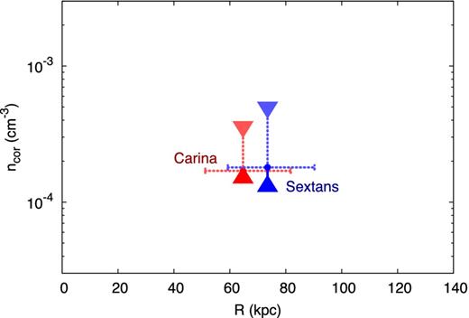
The families of orbits for each dSph are classified in terms of the pericentric radius (rp) and the velocity at pericentre (vp). We select only the orbits having pericentric passages compatible with our estimate of look-back time of the last burst of star formation tlb (see Section 3.3). In practice, given tlb and the width of the last SFR temporal bin, we accept only the orbits which have a pericentric passage within this bin. Fig. 1 shows the distribution of these orbits in the (rp, vp) space. Given the non-triviality of this distribution, we decide to focus on three representative orbits. The median orbit is given by the median value of the pericentric radius |$\bar{r}_{\rm p}$| and the median of |$\bar{v}_{\rm p}$| in the range ±3 kpc around |$\bar{r}_{\rm p}$|. For Sextans, we obtain |$\bar{r}_{\rm p}=59.8\,\,{\rm kpc}$| and |$\bar{v}_{\rm p}=270.4 \,{\rm km\,s}^{-1}$|, in agreement with the values obtained by Lux et al. (2010) for the last pericentric passage. We then select two more orbits at the first and third quartiles of the distribution of rp and their corresponding values of vp. The selected orbits are indicated by the large diamonds in Fig. 1.
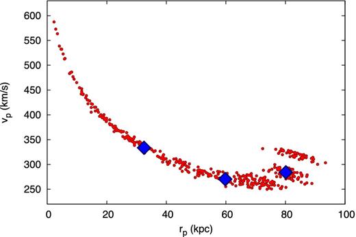
Pericentric radii and velocities for the orbits of the Sextans dSph compatible with a pericentric passage at the stripping time (tlb) determined from the SFH (see the text). The large (blue) diamonds show the three representative orbits (median, first and third quartiles in rp and in vp within ±3 kpc from the selected value of rp) chosen for our simulations.
Thus, as far as the orbits are concerned, we perform three distinct sets of hydrodynamical simulations. The parameters of the three representative orbits for Sextans are reported in Table 5. We show in Section 4.2 that the results for Sextans’ orbits are remarkably consistent with each other despite the large difference in their input parameters. This is an encouraging test of our model assumptions and systematics. Given these results, we consider only the median orbit for Carina.
3.3 Initial gas distribution
In our simulations, the ISM of the dwarf galaxies is composed by isothermal (T = 104 K) gas that is in hydrostatic equilibrium with the DM potential and has a subsolar metallicity taken from the literature (see Table 4). Note that the metallicity of the coronal gas is always set to 0.1 Z⊙ (see Section 3.1). The radius at which the cold gas distribution is truncated corresponds to the radius where its pressure is equal to the pressure of the coronal gas. The latter depends on the coronal temperature, for which we explore different values, Tcor = 1, 1.8, 3 × 10⁶ K (see again Sections 3.1 and 4.4). Since the gravitational potential of the DM halo is fixed, the gas density distribution in the dwarf is fully determined once we set the central density. We estimate this central density using information contained in the SFH, as described below.
We derived the look-back time of the last burst of star formation (tlb) as the time when the estimated value of the SFR is consistent with zero within the given uncertainties. At that time, we assume that the dwarf has a negligible amount of gas left, i.e. we consider the gas stripping process as completed. In Table 1, we report the times of the last stripping event for the dSphs. We refer to this as the last stripping event because it is likely that dSphs have suffered gas stripping also at earlier times. Considering only the last event has a number of advantages: (i) it saves computational time, (ii) it allows us to probe the corona at the closest possible look-back time and (iii) most importantly, it allows for the best possible reconstruction of the orbital paths (see Section 3.2).
Physical properties of the Carina and Sextans dSph galaxies. From left to right, the columns show the distance to the dwarf, the V-band luminosity, the pericentre and apocentre, the orbital period, the radius to the last measured kinematic data point rlast, the mass within rlast and the time to the last star formation burst tlb. Data are taken from Mateo (1998) (distance, LV), Walker et al. (2009) [rlast, MDM(rlast)] and Lux et al. (2010) (rp, ra, torb). tlb has been derived from the SFHs in Lee et al. (2009) (Sextans) and Rizzi et al. (2003) (Carina).
| dSph | Distance | LV | rp | ra | torb | rlast | MDM(rlast) | tlb |
|---|---|---|---|---|---|---|---|---|
| (kpc) | (106 L⊙) | (kpc) | (kpc) | (Gyr) | (kpc) | (107 M⊙) | (Gyr) | |
| Sextans | 86 ± 4 | 0.5 | 60 ± 20 | 200 ± 100 | 4 ± 3 | 1 | 2 | ∼7 |
| Carina | 101 ± 5 | 0.43 | 50 ± 30 | 110 ± 30 | 1.8 ± 0.8 | 0.87 | 3.7 | ∼0.5 |
The SFHs of Sextans and Carina, taken from Lee et al. (2009) and Rizzi et al. (2003), are shown in Fig. 2. The look-back times of the last starburst (i.e. the last stripping event) are tlb ∼ 7 and 0.5 Gyr, respectively. From the SFHs we can then extract the SFRs at the time prior to this event. These values are reported in Table 2.

Star formation properties and derived cold gas content of our two dSphs at the time of the last ram-pressure stripping event. The SFRs and gas density distributions are used as initial conditions for our hydrodynamical simulations. From left to right, the columns show the radius at which the SFR has been extrapolated, time to the last star formation burst, star formation rate at tlb, SFR surface density at tlb|$\Sigma _{\rm SFR}=\mathrm{SFR}/(\pi r_\mathrm{SF}^2)$|, initial mean cold gas density, initial central gas density, computed radius of the cold gas distribution and computed initial cold gas mass within rgas.
| dSph | rSF | tlb | SFR | ΣSFR | |$\bar{n}_{\rm gas}$| | n0, gas | rgas | Mgas |
|---|---|---|---|---|---|---|---|---|
| (kpc) | (Gyr) | (M⊙ yr−1) | (M⊙ yr−1 kpc−2) | ( cm−3) | ( cm−3) | (kpc) | ( M⊙) | |
| Sextans | 0.5 | 7 | 4.6 ± 2.2 × 10⁻⁵ | 5.9 × 10⁻⁵ | 0.09 | 0.27 | 0.98 | 7 × 10⁶ |
| Carina | 0.28 | 0.5 | 4.6 ± 1.3 × 10⁻⁶ | 1.9 × 10⁻⁵ | 0.14 | 0.4 | 0.4 | 6.3 × 10⁵ |
There are two key uncertainties related to our reconstruction of the SFR at a given look-back time.
The time resolution of the SFH makes the tlb uncertain by about 0.5–1 Gyr. This is a small error compared to other uncertainties.
The presence of ‘blue straggler stars’ may contaminate the SFH, masquerading as recent star formation. Lee et al. (2009) explicitly consider this, publishing an alternate ‘corrected’ SFH for Sextans. The corrected SFH has no star formation at t > tlb and a small reduction in star formation at tlb. We preferred to use the uncorrected SFH shown in Fig. 2 because it is consistent with the one used for Carina (where the correction has not been applied). However, we explicitly tested for the effect of blue straggler contamination on our results by running some additional simulations using the corrected SFH of Lee et al. (2009). We found that the final value of the coronal density does not vary appreciably within our quoted uncertainties.
Once we know the SFR before stripping, we use a revised version of the KS relation to estimate the gas density at that time. The standard KS relation connects the (molecular and atomic) hydrogen surface density, |$\Sigma _\mathrm{H\,{\small I}}$| and |$\Sigma _\mathrm{H_2}$|, and the SFR surface density, ΣSFR, with a power law (slope 1.4). It is valid for disc galaxies and starburst galaxies (e.g., Kennicutt 1998a). It is well known that this relation steepens considerably for column densities below ∼10 M⊙ pc−2 (e.g. Leroy et al. 2008). While the ΣSFR seems to correlate very well with the molecular gas surface density (Bigiel et al. 2011), the relation breaks down at low densities likely due to the transition from a molecular-dominated to an atomic-dominated ISM (Krumholz, Dekel & McKee 2012). Due to the low values of the SFRs of our dwarfs (see Table 2), the expected |$\Sigma _\mathrm{H\,{\small {I}}+H_2}$| falls below the limit and the dwarfs’ ISM is dominated by H i, as confirmed by observations (see Table 3 and references therein). In this paper, we do not distinguish between different gas phases in the ISM as in the simulations the cooling is truncated at 104 K. This is an acceptable approximation since our star formation and feedback prescriptions are purely empirical and based on the observed SFR.
To make sure that equation (10) is suitable for our purposes, we check that it holds for galaxies in the Local Group. We consider four dIrrs that span a large range of gas and SFR surface densities. For each of them, we calculate ΣSFR knowing the value of the SFR and the area of the galaxy from which it has been derived. We then estimate the surface densities of H i and molecular gas (when present) averaged over the same area. The obtained values are listed in Table 3. As expected, the molecular phase plays a minor role and can safely be neglected. In Fig. 3, we show the obtained values of ΣSFR and |$\Sigma _\mathrm{H{\,\small {I}}}$| (solid circles), as well as the relation from equation (10). The agreement is remarkably good for all the dIrrs; the dashed lines show the 1σ error. Note that the standard KS relation (dashed line) would clearly overestimate ΣSFR at these gas surface densities by up to an order of magnitude.

SFR densities and gas densities for four dIrrs of the Local Group. CO is not detected in Wolf–Lundmark–Melotte (WLM) galaxy, and there is only an upper limit, while for Leo A and Leo T such studies are missing in the literature. References to the SFR, H i and CO studies (when applicable): (1) Efremova et al. (2011), (2) de Blok & Walter (2006), (3) Israel (1997), (4) Dolphin (2000), (5) Kepley et al. (2007), (6) Taylor & Klein (2001), (7) Cole et al. (2007), (8) Young & Lo (1996), (9) de Jong et al. (2008) and (10) Ryan-Weber et al. (2008).
| Galaxy | ΣSFR | |$\Sigma _\mathrm{H{\,\small {I}}}$| | |$\Sigma _\mathrm{H_2}$| | Ref. |
|---|---|---|---|---|
| (M⊙ yr−1 kpc−2) | ( M⊙ pc−2) | |||
| NGC 6822 | 2.15 × 10⁻³ | 7.6 | 1.1 | (1, 2, 3) |
| WLM | 1.2 × 10⁻³ | 6.5 | Negligible | (4, 5, 6) |
| Leo A | 1.1 × 10⁻³ | 4.8 | Missing | (7, 8) |
| Leo T | 4.4 × 10⁻⁵ | 1.5 | Missing | (9, 10) |
3.4 Radiative cooling, star formation and feedback
Radiative cooling is included in the code by taking the collisional ionization equilibrium cooling function of Sutherland & Dopita (1993). The cooling term is added explicitly to the energy equation of the gas and, for stability reasons, the hydrodynamic time-step is reduced to 10 per cent of the minimum cooling time in the computational domain. Metal cooling is taken into account and the metallicity of the gas is treated as a passive scalar field advected by the flow. The cooling rate is set to zero below Tmin = 104 K.
We include star formation in our hydrodynamical code by introducing a temperature cut, Tcut = 4 × 10⁴ K. Only cells below this temperature are allowed to form stars. The amount of gas converted into stars is computed from equation (10), where the gas density is a function of time. However, given that the star formation rates used for our simulated dwarfs are small (see Table 2), there is no significant depletion of gas. This is an important point as it shows that the removal of gas from Sextans and Carina cannot be achieved by star formation alone. Rather, it requires additional processes, i.e. a combination of SN feedback and gas stripping.
Concerning SN explosions, we assume that our SN bubbles start their expansion at the end of the adiabatic (Sedov) phase and we only follow the subsequent radiative phase. In this phase, the thermal energy is lost due to radiative cooling and adiabatic expansion, while the kinetic energy is used partially for the expansion and partially it is transferred to the ambient medium at later times. The explosion of a single SN is implemented by increasing the volumetric thermal energy density by a factor |$\frac{E_\mathrm{SN}}{V_\mathrm{Sedov}}$|, where ESN = 1051 erg and |$V_\mathrm{Sedov}=\frac{4}{3}\pi r_\mathrm{Sedov}^3$| represents the initial spherical volume of the bubble, with rSedov the radius of the injection region. For every different gas profile, rSedov – the SN bubble radius at the end of the adiabatic phase – is determined by running very high resolution simulations of a single SN exploding in the centre of the dwarf. rSedov is then set to the value of the initial radius that produces a match between the simulated evolution of the SN shock radius and the analytical (two-dimensional) one for the radiative phase. We model a SN bubble at the explosion time with just four cells, since higher numbers cause our simulations to be too demanding from a numerical point of view. Thus, the resolution of a simulation is defined by the value of rSedov by simply equating the circular area of the SN bubble with the Cartesian one of four cells. We also adopt the overcooling correction method described in Anninos & Norman (1994).
We compute the supernova rate (SNR) from the SFR using the initial mass function (IMF) Ψ(M) chosen to retrieve the SFH of our dwarf galaxies. For Sextans and Carina, a Salpeter IMF (Salpeter 1955) was assumed (see Rizzi et al. 2003; Lee et al. 2009). In this case, |$\mathrm{SNR}\simeq \frac{6\times 10^{-3}}{\rm M_{\odot }}\mathrm{SFR}$||$\frac{\mathrm{SN}}{\mathrm{yr}}$|, with the SFR expressed as M⊙ yr−1. Applying for the SFR found in every cell with T < Tcut and multiplying the obtained SNR with the time-step, we find the number of SN ‘events’ occurring in each cell during a given time-step. From this, we can then generate random explosions across the dwarf galaxy. Note that, since the SFR of the simulation is tied to the dwarf's gas, the SNR is dependent on the amount of cold gas at that specific time-step, assuming that the SNe form and explode instantaneously. Using this method the SNR in a simulation of a dwarf in isolation (without the ‘coronal wind’) is recovered within ∼10 per cent of the expected value.4
3.5 Simulations setup
In Table 4, we list the details of our main runs. Different initial conditions for the dwarfs are computed by exploring the main model uncertainties: the orbit reconstruction, the determination of the SFH and the star formation law (see Section 4.2). Each set of runs for the two dwarfs has been simulated many times by changing the value of ncor (which sets the dwarf's gas truncation radius rgas and initial mass Mgas once the central gas density is fixed) until complete gas stripping occurs at the end of the simulation. We consider that a galaxy is devoid of gas when the mass of cold (T < 1 × 10⁵ K) gas bound to the potential of the dwarf is <5 per cent of the initial mass. The remaining small amount of cold gas can be easily stripped in the following part of the orbit. Large sizes of the computational box are needed to avoid boundary effects (such as reflected waves) on the surface of the dwarf. The boundaries used are ‘Wind’ in the x-direction (‘Inflow’ on the right side and ‘Outflow’ on the left one) and ‘Outflow’ in the y-direction. The velocity of the inflow is set according to the selected orbits. Δr (and the corresponding Δt) is determined by the orbit's choice, and it represents the range of distances from the MW over which the recovered coronal density has effectively been averaged. Such values have been determined using equation (9) with a stripping efficiency of 50 per cent (see Section 3.2).
Parameters of the simulations. Each run is denoted by the dwarf name, the initial density of the dwarf's ISM (see Sections 3.3 and 4.2), the pericentric distance of the orbit and the temperature of the corona (if different from the reference value Tcor = 1.8 × 10⁶ K). Lbox is the size of the computational domain in each direction, Δx is the resolution, Tcor is the coronal temperature, n0, gas is the initial central density of the dwarf, Z is the dwarf's gas metallicity, |$\overline{v}_{\rm sat}$| is the dwarf velocity averaged over the simulated distance range Δr and Δt is the integration time corresponding to the part of the orbits with stripping efficiency greater than 50 per cent.
| Run | Lbox | Δx | Tcor | n0, gas | Z | |$\overline{v}_{\rm sat}$| | Δr | Δt |
|---|---|---|---|---|---|---|---|---|
| (kpc) | (pc) | (K) | ( cm−3) | (Z⊙) | (km s−1) | (kpc) | (Myr) | |
| SextansMidMed | 80 | 34 | 1.8 × 10⁶ | 0.27 | 0.02 | 228 | 59.8–90.2 | 930 |
| SextansLowMed | 80 | 39 | 1.8 × 10⁶ | 0.18 | 0.02 | 228 | 59.8–90.2 | 930 |
| SextansMid1stQ | 60 | 34 | 1.8 × 10⁶ | 0.27 | 0.02 | 286 | 33.9–59.2 | 420 |
| SextansLow1stQ | 60 | 39 | 1.8 × 10⁶ | 0.18 | 0.02 | 286 | 33.9–59.2 | 420 |
| SextansMid3rdQ | 100 | 34 | 1.8 × 10⁶ | 0.27 | 0.02 | 246 | 80.4–131.5 | 1220 |
| SextansLow3rdQ | 100 | 39 | 1.8 × 10⁶ | 0.18 | 0.02 | 246 | 80.4–131.5 | 1220 |
| CarinaMidMed | 80 | 31 | 1.8 × 10⁶ | 0.4 | 0.01 | 251 | 51.2–81.8 | 740 |
| CarinaLowMed | 80 | 35 | 1.8 × 10⁶ | 0.31 | 0.01 | 251 | 51.2–81.8 | 740 |
| CarinaMidMed1e6K | 80 | 31 | 1 × 10⁶ | 0.4 | 0.01 | 251 | 51.2–81.8 | 740 |
| CarinaMidMed3e6K | 80 | 31 | 3 × 10⁶ | 0.4 | 0.01 | 251 | 51.2–81.8 | 740 |
4 RESULTS
In Section 4.1, we describe our fiducial simulation setup for Sextans, which has been obtained by taking the orbit with the median value of the pericentric distance |$\bar{r}_{\rm p}$|. For this fiducial setup, we illustrate the principal results of our analysis, in particular the procedure that we adopted to determine the coronal density (averaged over the distance range encompassed by the orbit) that produces complete stripping of the dwarf's ISM. We examine, in Section 4.2, how the estimate for the coronal density is affected by the choice of the orbit and the uncertainties in the initial conditions. In Section 4.3, we compare the values for the coronal density that we infer from Carina's simulations with those found for Sextans, and in Section 4.4 we show how the choice of different temperatures for the coronal gas affects the results.
4.1 Ram-pressure stripping from Sextans
We first examine the stripping of Sextans with the orbit parametrized by |$\bar{r}_{\rm p}=59.8 \,{\rm kpc}$| (see Section 3.2) and all other parameters as quoted in Tables 1 and 2 and in the first line of Table 4, which represents our fiducial setup. We then run a series of simulations varying only the mean coronal density ncor until we find the value that produces complete stripping of gas within the time of the simulation. We find that the minimum coronal density needed for stripping to occur is ncor|min = 1.8 × 10⁻⁴ cm−3.
Fig. 4 shows the temperature distribution at times t = 0, 240, 470, 700, 730, 930 Myr. We see that, as the dwarf galaxy starts to experience the ram pressure exerted by the corona, a wake of stripped gas is formed. This wake becomes progressively more elongated and structured as time passes. In this wake, knots of cold gas (T ∼ 104 K) and regions at intermediate temperatures (∼105 K) coexist. The presence of these intermediate-temperature regions is indicative of a mixing between the stripped dwarf's ISM and the coronal material. The gas removal is not an instantaneous process. The mass-loss rate is initially rather low and increases after the dwarf has passed the orbit pericentre. In Fig. 5, we show the evolution of the mass of the cold gas mass bound to Sextans (i.e. all gas with velocity less than the local escape velocity and T < 105 K). The mass of bound gas decreases steadily and at an increasing rate throughout the simulation. The increasing mass-loss rate is a result of the progressive disruption of the dwarf by ram-pressure stripping assisted by SN feedback. Before the pericentre, only roughly 20 per cent of the gas is lost, and the other 80 per cent is lost in the second half of the simulation. Approximately 1 Gyr is required to reach a final mass of cold, bound gas of ∼5 × 10⁴ M⊙, ∼1 per cent of the initial one.
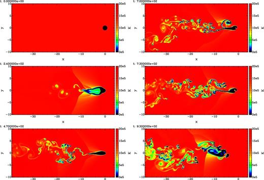
Time evolution of the temperature distribution for our fiducial setup for the Sextans dSph with ncor = 1.8 × 10⁻⁴ cm−3. In the left column (top to bottom), we show t = 0, 240 and 470 Myr, and in the right column we plot t = 700, 730 and 930 Myr. The bottom-left panel corresponds roughly to the time of pericentric passage. We only show a small section of the box. The axes are given in kpc.
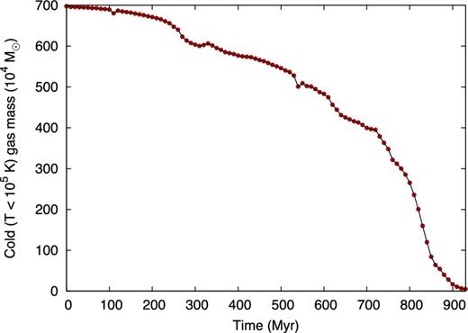
Mass of cold (<105 K) gas gravitationally bound to the DM halo of Sextans as a function of time from the beginning of our fiducial simulation. The pericentre passage occurs at t = 465 Myr.
4.2 Coronal gas density: lower bounds, errors and upper bounds
To reliably estimate the MW's coronal density, different sets of initial conditions must be explored to account for various uncertainties. The main model uncertainties are due to the orbit reconstruction, the determination of the SFH and the star formation law. In this section, we consider in turn each of them.
We start with the uncertainties in the orbit determination. Fig. 6 shows the minimum values of the density of the MW's corona (points) that produce complete stripping from Sextans for the three representative orbits chosen in Section 3.2, i.e. the median value of rp and the first and third quartiles of its distribution. The error bar in the radius represents the range over which the coronal density has to be considered average (see Table 4, eighth column, rows 1, 3 and 5, labelled as ‘mid’), while the derivation of the lower errors and the upper limits to the coronal density is described below. The orbital parameters used to derive the coronal densities shown in Fig. 6 are quite different (see Fig. 1 and Section 3.2). Nevertheless, the density required for the stripping is similar for the three orbits and shows a nice decreasing trend with the distance from the MW. This shows that the value of the coronal density is not too sensitive to the specific choice of the orbital parameters. The resulting values for ncor|min are reported in Table 5 labelled as ‘mid’.
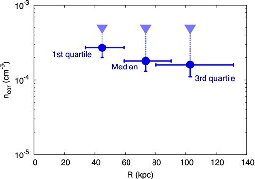
Density of the corona of the MW that produces complete gas stripping from the Sextans dSph. The different determinations refer to three representative orbits for the dSph with different pericentric radii, i.e. the median orbit, and the first and third quartiles of the distribution of pericentric radii. The down-pointing triangles show upper limits referred to that specific radius. The derivation of errors and upper limits is described in the text (Section 4.2).
Simulations that produced the complete stripping of gas from the dSphs. The labels ‘mid’ and ‘low’ refer to the initial density of the dwarf's ISM. rp is the pericentre distance of the simulations, Δr is the considered spatial range from the pericentre found considering a stripping efficiency greater than 50 per cent (see also Table 4), vp is the velocity at the pericentre, Δtlb is the simulation time and ncor|min is the inferred minimum average coronal density needed for stripping.
| dSph | rp | Δr | vp | Δtlb | ncor|min |
|---|---|---|---|---|---|
| point | (kpc) | (kpc) | (km s−1) | (Gyr) | ( cm−3) |
| Sextans | |||||
| mid | 59.8 | 30.4 | 270.4 | 0.93 | 1.8 × 10⁻⁴ |
| low | 59.8 | 30.4 | 270.4 | 0.93 | 1.3 × 10⁻⁴ |
| mid | 33.9 | 25.3 | 333.6 | 0.42 | 2.7 × 10⁻⁴ |
| low | 33.9 | 25.3 | 333.6 | 0.42 | 2 × 10⁻⁴ |
| mid | 80.4 | 51.1 | 284.1 | 1.22 | 1.6 × 10⁻⁴ |
| low | 80.4 | 51.1 | 284.1 | 1.22 | 1.1 × 10⁻⁴ |
| Carina | |||||
| mid | 51.2 | 30.6 | 291.4 | 0.74 | 1.7 × 10⁻⁴ |
| low | 51.2 | 30.6 | 291.4 | 0.74 | 1.5 × 10⁻⁴ |
Next we explore both the effect of the uncertainties on the measured SFH and on the applied star formation relation (equation 10), which influence the value of initial gas density of the dwarf, n0, gas. To investigate the effect of a lower dwarf ISM density, we run an additional set of simulations (labelled as ‘low’ in Tables 4 and 5). We derive the lower limit of the initial dwarf ISM density from an SFR of 2.4 × 10⁻⁵ M⊙ yr−1, corresponding to reducing the fiducial value of 4.6 × 10⁻⁵ M⊙ yr−1 by 1σ (see Table 2). We then use equation (10) with the upper +0.6 error to recover the lower n0, gas = 0.18 cm−3, which is shown in rows 2, 4 and 6 of Table 4. This gives a lower boundary for the coronal density which lies about 1σ below the fiducial value ncor = 1.8 × 10⁻⁴ cm−3. These values represent the lower error bars in Fig. 6 for the different orbits.
The above gives us a robust lower bound on the hot corona density. As outlined in Section 2.2, we additionally use pressure equilibrium to estimate an upper bound ncor|max by setting the gas truncation radius rgas equal to the star formation radius rSF. In doing this, we are neglecting any conspicuous redistribution of stars after tlb. We plot the resulting upper limits as downward-pointing triangles in Fig. 6. Given the (large) uncertainties – particularly on the orbit of Sextans – it is quite remarkable that all the values of the coronal density derived here appear to be consistent with one another.
4.3 Carina
We carry out a comparable set of simulations for the Carina dSph. For this dwarf we use only one orbit, i.e. that with median rp = 51.2 kpc, for which we find ncor|min = 1.7 × 10⁻⁴ cm−3. Estimating the lower error as before brings the lower limit down to ncor|min = 1.5 × 10⁻⁴ cm−3 (Table 5).
We compare the coronal densities of the MW derived by using the median orbit of Sextans and Carina in Fig. 7. As in Fig. 6, the horizontal bar represents the range in radii that we have considered for the simulation. We now use upward-pointing triangles placed at the location of the lower 1σ error to denote our lower bound. The upper limits (downward-pointing triangles) are estimated with the method described in Section 4.2. The derived values for the coronal density are reported in Table 5, while in Table 6 we list the ranges of the radii and the upper and lower bounds of the coronal density obtained for the median orbits of Sextans and Carina. The two dSphs have rather different structural properties and orbital parameters (see again Tables 1, 2 and 4) and yet there is a remarkable consistency for the recovered density values in the range of radii in which the two orbits overlap. This fact further supports the basic soundness of the methodology that we adopt here. Note in particular that the times of the last stripping (tlb) for the two dwarfs are very different. This may be an indication that the density of the Galactic corona has not changed significantly in the last ∼7 Gyr. Note also that the assumption that there has been no significant redistribution of the stellar component within the dwarf should be fully justified for Carina where tlb is only 0.5 Gyr.
Ranges of gas densities of the MW's corona allowed by the Sextans (blue) and Carina (red) dwarfs. The derivation of the lower and upper bounds (triangles) is described in the text (Section 4.2).
Average density of the MW corona together with its upper and lower limits as derived from the ram-pressure stripping along the median orbits of Sextans and Carina.
| Radius | Range | ncor|min | ncor|max |
|---|---|---|---|
| (kpc) | (kpc) | (cm−3) | (cm−3) |
| 73.5 | 59.8–90.2 | 1.3 × 10⁻⁴ | 5 × 10⁻⁴ |
| 64.7 | 51.2–81.8 | 1.5 × 10⁻⁴ | 3.6 × 10⁻⁴ |
| Radius | Range | ncor|min | ncor|max |
|---|---|---|---|
| (kpc) | (kpc) | (cm−3) | (cm−3) |
| 73.5 | 59.8–90.2 | 1.3 × 10⁻⁴ | 5 × 10⁻⁴ |
| 64.7 | 51.2–81.8 | 1.5 × 10⁻⁴ | 3.6 × 10⁻⁴ |
As a final end-to-end test of our systematic error, we consider a pericentric passage at the peak of the SFH of Carina. By matching ρgas with the value extracted from the following bin of the SFH, we derive a Galactic corona density approximately three times larger than using tlb. It is possible that this systematic shift implies some evolution in Carina's orbit over time; this interpretation will be considered in more detail in a separate forthcoming paper. Here, we simply note that even this extreme test results in a systematic error that is comparable to our other uncertainties.
4.4 Varying the coronal temperature
One of the main assumptions of our investigation is the temperature of the corona at the location of the dwarf galaxies. To study the effect of different coronal temperatures, we run additional simulations using the median orbit of Carina with the same parameters used before but different Tcor. In particular, we explore two additional coronal temperatures at Tcor = 3 × 10⁶ and 1 × 10⁶ K. The corresponding results, averaged over the range 51 < r < 82 kpc from the MW, are ncor, 3|min = 1.5 × 10⁻⁴ cm−3 and ncor, 1|min = 2.5 × 10⁻⁴ cm−3. The increase (decrease) of the coronal temperature causes the density to be lower (higher) than our fiducial value. In Section 5.1, we discuss the implications of these results for the missing baryon problem.
5 DISCUSSION
5.1 Missing baryons and the MW's corona
The results for the coronal density necessary for the stripping of gas from Sextans and Carina are summarized in Table 6. Here we show a conservative lower bound (fiducial value − lower error) and the upper bound determined in Section 2.2. We conclude that the coronal density, being a monotonic decreasing function of R, averaged between 50 and 90 kpc must be in the range 1.3 × 10⁻⁴ < ncor < 3.6 × 10⁻⁴ cm−3, consistent both with the detection claims by Gupta et al. (2012) and with the analytical estimates of Grcevich & Putman (2009). We recall that ncor is the total gas density ni + ne. The lower limit is computed by subtracting the average 1σ of Sextans and Carina lower values to the value of the coronal density (ncor = 1.75 × 10⁻⁴ cm−3) determined by averaging our fiducial ‘mid’ simulations (Table 5).
It is possible to use our derived range of ncor as a constraint for the global density profile of the MW's corona. This profile is obtained by following the procedure outlined in Section 2.4. From the density profile, one can extrapolate the total mass of the corona within the virial radius of the MW, which can then be compared to the missing baryonic mass of the Galaxy. In addition to ncor, we take also into account two further constraints discussed in AB10:
the dispersion measures along the line of sight to Large Magellanic Cloud (LMC) pulsars, from which AB10 estimate an upper bound for the coronal density of |$\overline{n}_{\mathrm{e}}=5\times 10^{-4} \,{\rm cm}^{-3}$| averaged over 50 kpc from the Galactic Centre;
the upper limit for X-ray emission measure, assuming our fiducial value of the coronal metallicity of 0.1 Z⊙.
The dispersion measure of LMC pulsars is the more stringent constraint at present due to our assumption of a low coronal metallicity.
Through equation (6), we compute a series of coronal density profiles consistent with all of the above constraints, using three different assumptions about the thermodynamic state of the coronal gas: isothermal (γ = 1), adiabatic (γ = 5/3) and ‘cooling’ (γ = 1.33). As for the DM potential we make two different choices: our default TF potential [see equation (6) truncated at5 10 ≤ R ≤ Rvir = 236 kpc, with Mvir = 1.54 × 10¹² M⊙] and an NFW profile. We also consider three different coronal temperatures: 1.8 × 10⁶, 106 and 3 × 10⁶ K. The exploration of the parameter space resulted in 21 models compatible with all of the constraints considered here. In particular, we find that, regardless of the choice of the potential, for the isothermal models our upper limits are less stringent than the constraint from the dispersion measure, while for the adiabatic and cooling coronae they are roughly coincident. Hence, the upper limits on the MW's baryon fraction described in this section are determined by the dispersion-measure limit rather than our pressure-confinement method described in Section 2.2.
To derive the expected mass of the missing baryons Mmb associated with the MW, we follow again AB10 and set Mmb = 15 per cent Mtot, where Mtot is the sum of the DM mass (Mvir) and the observed baryon mass. For the latter, we take Mob = 6 × 10¹⁰ M⊙ (see Section 1). The expected missing baryonic mass is then 2.4 × 10¹¹ M⊙ for the TF model.
Our results are presented in Fig. 8, where we show the ranges given by Sextans and Carina and the coronal profiles with reference values ncor = 1.75 × 10⁻⁴ and 1.5 × 10⁻⁴ cm−3 for Tcor = 1.8 × 10⁶ and 3 × 10⁶ K, respectively. All the models with Tcor = 106 K yielded no solution consistent with all of the constraints and therefore are not shown. In the isothermal case, we find for Tcor = 1.8 × 10⁶ K (3 × 10⁶ K) a coronal baryon fraction of 15–20 per cent (22–50 per cent) of the expected MW's missing baryons, marginalizing over all uncertainties. For adiabatic and ‘cooling’ models instead, the temperature profile is no longer constant and so our assumed coronal temperature corresponds to an average over the ranges 50-90 and 50–80 kpc for Tcor = 1.8 × 10⁶ and Tcor = 3 × 10⁶ K, respectively. The results for an adiabatic or ‘cooling’ halo are nearly indistinguishable, with a difference of ≲ 2 per cent in the recovered missing baryon fractions. For Tcor(50–90 kpc) = 1.8 × 10⁶ K, we find a coronal baryon fraction of 16–48 per cent of the expected missing baryons, while for Tcor(50–80 kpc) = 3 × 10⁶ K the value is 26–100 per cent. As expected, for an adiabatic or ‘cooling’ corona, the baryon fraction can be significantly larger than in the isothermal case because the density in such a corona drops less rapidly with radius, allowing more gas to be stored in the huge volume just inside the virial radius. An adiabatic corona at high temperature could, in principle, contain all of the MW's expected missing baryonic mass. These results are broadly consistent with those of AB10 and also the estimates of missing baryon fractions in external galaxies (Anderson & Bregman 2011; Dai et al. 2012; Anderson, Bregman & Dai 2013), although our fractions are higher than theirs probably due to our lower value of the coronal metallicity.
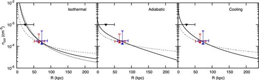
Density profiles for different coronal models consistent with all constraints: the range of coronal densities allowed by our analysis for Sextans and Carina, pulsar dispersion measures (black triangle) and X-ray emission upper limits (not shown). The solid line corresponds to Tcor(50–90 kpc) = 1.8 × 10⁶ K and the dashed line to Tcor(50–80 kpc) = 3 × 10⁶ K. The dotted line in the left-hand panel shows results for an NFW potential (as opposed to our default TF potential). From left to right, panels consider an isothermal (γ = 1), adiabatic (γ = 5/3) and ‘cooling’ (γ = 1.33) halo.
Finally, we consider how our assumption of a TF profile affects these results. We use instead the NFW potential from AB10 with Rvir = 250 kpc, Mvir = 2 × 10¹² M⊙ and concentration parameter c = 12 (see the dotted line, left-hand panel of Fig. 8). Note that for an NFW profile, the gas density falls more steeply leading to a lower extrapolated total mass. However, the effect is typically quite small compared to the other uncertainties. Our results for the missing baryon fractions are summarized in Table 7. All isothermal models predict an amount of missing baryons in the corona between 10 and 50 per cent of the expected value (see also Miller & Bregman 2013). If the hot gas has an adiabatic equation of state, the corona can accommodate more gas and we cannot rule out that it could contain the whole predicted amount of missing baryons (see also Fang et al. 2013).
The fraction and mass of the missing baryons contained in coronae for different combinations of coronal temperature, equation of state and Galactic potential consistent with the observational constraints.
| Potential | Tcor | | $ \frac{{M\left( { < r_{{\rm vir}} } \right)}}{{M_{{\rm mb}} }}$| | | $ \frac{{M\left( { < r_{{\rm vir}} } \right)}}{{M_ \odot }}$| | ||
|---|---|---|---|---|---|
| – | (106K) | Isothermal | Adiabatic | Isothermal | Adiabatic |
| TF | 1.8 | 15–20 per cent | 16–48 per cent | 3.6 × 10¹⁰–4.8 × 10¹⁰ | 3.8 × 10¹⁰–1.1 × 10¹¹ |
| NFW | 1.8 | 11 per cent | 9–25 per cent | 3.4 × 10¹⁰ | 2.8 × 10¹⁰–7.7 × 10¹⁰ |
| TF | 3.0 | 22–50 per cent | 26–100 per cent | 5.3 × 10¹⁰–1.2 × 10¹¹ | 6.2 × 10¹⁰–2.4 × 10¹¹ |
| NFW | 3.0 | 16–33 per cent | 18–74 per cent | 4.5 × 10¹⁰–1011 | 5.6 × 10¹⁰–2.3 × 10¹¹ |
5.2 Comparison with the analytic ram-pressure stripping formula
| Point | nan | nsim | |$\overline{n}_\mathrm{gas}$| | |$\overline{v}_{x}$| |
|---|---|---|---|---|
| ( cm−3) | ( cm−3) | ( cm−3) | ( km s−1) | |
| Sextans | ||||
| Median | 3.6 × 10⁻⁵ | 1.8 × 10⁻⁴ | 0.09 | 228 |
| First quartile | 2.3 × 10⁻⁵ | 2.7 × 10⁻⁴ | 0.09 | 286 |
| Third quartile | 3.1 × 10⁻⁵ | 1.6 × 10⁻⁴ | 0.09 | 246 |
| Carina | ||||
| Median | 3.2 × 10⁻⁵ | 1.7 × 10⁻⁴ | 0.14 | 251 |
5.3 SN feedback
One of the novel features of this work is the introduction of discrete SN injections. If we do not consider SN explosions, the stripping process should naturally evolve towards a Kelvin–Helmholtz (KH) assisted regime. Additionally, the fact that we are using a varying dwarf velocity means that we expect the development of Rayleigh–Taylor (RT) instabilities. However, SN explosions are very efficient at changing the local morphology of the gas distribution, leading to an effective disruption of the RT/KH seeds. In practice, SNe destroy the regular flow at the interface between the hot and cold gas, leading to an SN-assisted stripping process. Without considering SN explosions, the gas flow past the dwarf is rather smooth and eddies form. Including SNe, as shown in Fig. 4, causes the flow to be quite clumpy. Perhaps, these cold clumps travelling at a few hundreds of km s−1 are related to (some of) the MW's HVCs (see also Mayer et al. 2006; Binney et al. 2009).
Figs 9 and 10 show the evolution of the cold bound mass and the cold mass-loss rate for the fiducial simulation of Sextans (median orbit and ncor = 1.8 × 10⁻⁴ cm−3) with and without SNe. SN explosions increase the cross-section of the cold gas distribution, leading to a more efficient stripping and a mass-loss rate that can become four times larger than that without SNe (see Fig. 10). On the other hand, the same simulation including SNe but without ram-pressure stripping leads to an inefficient gas removal process, with a final cold gas mass very close to the initial one. For this reason, we conclude that it is the combination of SNe and ram pressure that is key for recovering the correct stripping rate. Without SNe, the coronal density required to completely strip away the gas is ncor|min = 2.9 × 10⁻⁴ cm−3 – about two times higher than for our reference simulation with SNe. This is higher than independent observational limits on the coronal density (see Section 5.1), suggesting that SN explosions are critical for recovering realistic coronal profiles (see also Nichols & Bland-Hawthorn 2011).
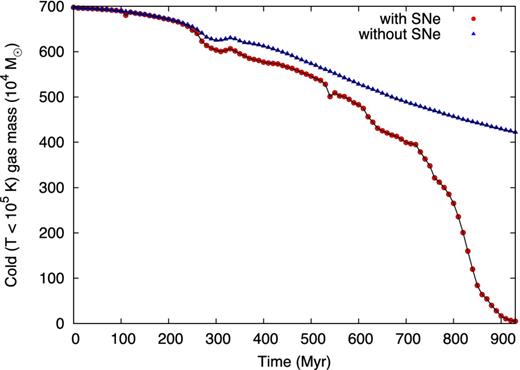
Cold, bound gas mass for the fiducial simulation of Sextans with and without SNe.
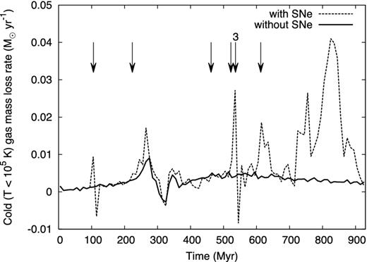
Cold gas mass-loss rates for the fiducial simulation of Sextans with and without SNe. The arrows represent the time at which an SN has exploded; the number 3 over the fifth arrow means that a burst has occurred (three SNe in 8 Myr).
6 CONCLUSIONS
We have performed a suite of hundreds of hydrodynamical simulations of ram-pressure stripping of two dwarfs, Sextans and Carina, in order to estimate a lower bound on the coronal gas density of the MW. In addition, we have derived an upper bound by considering the pressure confinement of these dwarfs by the hot corona. We have introduced several novel features as compared to previous analyses: realistic orbits for the dwarfs, a model of discrete SN feedback and a recovery of the initial gas mass contained in the dwarfs (determined from their measured SFHs). We find that the coronal number density in the range 50-90 kpc from the Galaxy must be in the range 1.3 × 10⁻⁴ < ncor < 3.6 × 10⁻⁴ cm−3. We have considered many sources of systematic and random error ensuring that this result is robust.
We have derived coronal models consistent with our lower and upper bounds on the coronal density, X-ray emission limits and pulsar dispersion measures. The pulsar constraint is particularly important in providing a more rigorous upper bound on the coronal density than our pressure-confinement calculation (that requires an additional assumption about the radial extent of star formation within the dSphs). We have explored different coronal temperatures, Galactic potentials and equations of state for the gas, computing a set of coronal density profiles consistent with all of the above constraints. Extrapolating the baryonic mass in these models to large radii, we have estimated the fraction of ‘missing baryons’ that can exist in a hot corona within the MW's virial radius. Considering as a reference model an isothermal corona at Tcor = 1.8 × 10⁶ K in hydrostatic equilibrium with the Galactic potential, the missing baryon fraction is 10–20 per cent. Hotter and/or adiabatic coronae can contain more baryons than our reference model. However, of the set of 21 coronal density profiles analysed in this work, only one model (hot and adiabatic) is consistent with all of the expected missing baryons lying within the virial radius of the MW. Thus, models for the MW must either explain why its corona is in a hot, adiabatic thermal state, or why a large fraction of the MW's baryons either never fell in or were removed by energetic feedback.
We thank an anonymous referee for comments and suggestions that improved the clarity of this work. We also thank E. Held and L. Rizzi for providing data, and M. Anderson, G. Battaglia, J. Binney, T. Naab and S. White for helpful comments and discussions. We acknowledge the CINECA awards N. HP10CPPUNB and HP10C8MF3E (2011), the ETHZ Brutus Cluster and the RZG Odin Cluster for the availability of high-performance computing resources and support. AG and SW thank the Deutsche Forschungsgemeinschaft (DFG) for funding through the SPP 1573 ‘The Physics of the Interstellar Medium’. FF acknowledges support from PRIN-MIUR, project ‘The Chemical and Dynamical Evolution of the Milky Way and Local Group Galaxies’, prot. 2011SPTACC. JIR would like to acknowledge support from SNF grant PP00P2_128540/1. FM is supported by the collaborative research centre ‘The Milky Way System’ (SFB 881) of the DFG through subproject A1. HL acknowledges a fellowship from the European Commission's Framework Programme 7, through the Marie Curie Initial Training Network CosmoComp (PITN-GA-2009-238356). The original idea for this work arose during the inspiring meeting ‘Problematik’ that took place at Magdalen College, Oxford (UK), in 2010 August.
Due to the poor knowledge of such a phase, this fraction has been assumed rather than measured.
To see why that is the case, note that in the limit ra ≫ rp, and assuming spherical symmetry, the pericentre of the dwarf orbit is completely determined by its specific angular momentum (e.g. Read et al. 2006a):
SNe alone are inefficient in removing the gas (see also Section 5.3). Thus, the SFR remains constant along the simulation and the simulated SNR can be compared with the predicted one. The match between the computed and the expected value (within 10 per cent) shows the viability of our implementation.
This inner truncation is used to avoid any contamination from the disc and does not affect the value of the recovered coronal mass (see also AB10).
