


Abstract
In this paper, globular star clusters which contain a subsystem of stellar mass black holes (BH) are investigated. This is done by considering two-component models, as these are the simplest approximation of more realistic multimass systems, where one component represents the BH population and the other represents all the other stars. These systems are found to undergo a long phase of evolution where the centre of the system is dominated by a dense BH subsystem. After mass segregation has driven most of the BH into a compact subsystem, the evolution of the BH subsystem is found to be influenced by the cluster in which it is contained. The BH subsystem evolves in such a way as to satisfy the energy demands of the whole cluster, just as the core of a one-component system must satisfy the energy demands of the whole cluster. The BH subsystem is found to exist for a significant amount of time. It takes approximately 10trh,i, where trh,i is the initial half-mass relaxation time, from the formation of the compact BH subsystem up until the time when 90 per cent of the subsystem total mass is lost (which is 103 times the half-mass relaxation time of the BH subsystem at its time of formation). Based on theoretical arguments, the rate of mass-loss from the BH subsystem (Ṁ2) is predicted to be −βζM/(αtrh), where M is the total mass, trh is the half-mass relaxation time and α, β, ζ are three dimensionless parameters (see Section 2 of the main text for details). An interesting consequence of this is that the rate of mass-loss from the BH subsystem is approximately independent of the stellar mass ratio (m2/m1) and the total mass ratio (M2/M1) (in the range m2/m1 ≳ 10 and M2/M1 ∼ 10−2, where m1 and m2 are the masses of individual low-mass and high-mass particles, respectively, and M1 and M2 are the corresponding total masses). The theory is found to be in reasonable agreement with most of the results of a series of N-body simulations, and with all of the models if the value of ζ is suitably adjusted. Predictions based on theoretical arguments are also made about the structure of BH subsystems. Other aspects of the evolution are also considered such as the conditions for the onset of gravothermal oscillation.
INTRODUCTION
Hundreds of stellar mass black holes (BH) can form within a massive globular cluster (see Kulkarni, Hut & McMillan 1993; Sigurdsson & Hernquist 1993; Portegies Zwart & McMillan 2000). Some of the BH might escape at the time of their formation due to large natal kicks. However, the subject of natal kicks for BH is still under debate (Repetto, Davies & Sigurdsson 2012) and it is possible that the largest BH may form without any supernova explosion (Fryer 1999). Uncertainty in the natal kicks leads to uncertainty in the initial size of the BH population. As the BH are more massive than the other stars in the system, any retained BH will undergo mass segregation and almost all are likely to become concentrated in the centre of the system, eventually forming a compact subsystem.
The mass of the BH subsystem decreases over time because BH binaries form in the dense core of the BH subsystem, causing the ejection of a single BH and ultimately the binaries themselves through superelastic encounters (see Kulkarni et al. 1993; Sigurdsson & Hernquist 1993; Portegies Zwart & McMillan 2000; Banerjee, Baumgardt & Kroupa 2010; Downing et al. 2010; Aarseth 2012). Early work by Kulkarni et al. (1993) and Sigurdsson & Hernquist (1993) seemed to indicate that the BH population will become depleted over a relatively short time-scale. This conclusion was reached in part by treating the BH subsystem as if it were an independent system once most of the BH had segregated to the centre of the cluster.
Merritt et al. (2004) and Mackey et al. (2008) found that heating by a retained population of BH causes large-scale core expansion in massive star clusters. They suggest that this may partly explain the core radius–age trend observed for such objects in the Magellanic Clouds. The BH binaries that are formed in the core of the BH subsystem are an interesting class of objects in their own right, especially as the merger of two BH may be detectable as a source of gravitational waves (Portegies Zwart & McMillan 2000; Banerjee et al. 2010). It has even been suggested that star clusters consisting almost entirely of BH, known as dark star clusters, could exist (Banerjee & Kroupa 2011). Dark star clusters could be created if the stars in the outer parts of a larger system were stripped away by a strong tidal field, leaving behind the BH subsystem. If one were to observe the few remaining stars in these systems, they would appear to be supervirial, as the velocity dispersion of the remaining stars would be enhanced by the unseen BH.
Breen & Heggie (2012a) investigated the evolution of two-component models and found that, within the parameter space they considered, the stability of the two-component system against gravothermal oscillations was dominated by the heavy component. They only considered systems with a total mass ratio of the order of M2/M1 ≳ 10−1, where M2 (M1) is the total mass of the heavy (light) component. However, the mass ratio of a system containing a BH subsystem would only be expected to be M2/M1 ∼ 10−2 (Portegies Zwart & McMillan 2000), where M2 is the total mass of the BH subsystem, which is smaller by an order of magnitude than any of the systems studied by Breen & Heggie (2012a). As Hénon's principle (Hénon 1975) states that the energy generating rate of the core is regulated by the bulk of the system, it seems unlikely that the approach of Breen & Heggie (2012a) is appropriate in this case due to the small value of M2/M1.
This paper is structured as follows. In Section 2, some theoretical results are derived and discussed. This is followed by Section 3, where the theoretical results regarding the size of the BH subsystem are tested using both gas models and direct N-body runs. Section 4 contains empirical results regarding the mass-loss rates from BH subsystems and a comparison between the empirical results and the theory of Section 2. The qualitative behaviour of these systems is also discussed in this section. Section 5 is concerned with gravothermal oscillations in systems containing a BH subsystem. Finally, Section 6 consists of the conclusions and a discussion.
THEORETICAL UNDERSTANDING
BH subsystem: half-mass radius
Here we will consider aspects of the dynamics of a system containing a BH subsystem. We will assume that the system is Spitzer unstable (Spitzer 1987) and that the total mass of the BH subsystem (M2) is very small compared to the total mass of the system (M). (Since the Spitzer stability criterion is |$(M_2/M_1)(m_2/m_1)^{\frac{3}{2}}< 0.16$|, these assumptions are consistent provided the stellar mass ratio m2/m1 is large enough.) We will also assume that the initial state of the system has a constant mass density ratio between the two components throughout and that the velocity dispersions of both components are equal at all locations. If this is the case, then the system would first experience a mass-segregation-dominated phase of evolution which lasts ∼ (m1/m2)tcc (Fregeau et al. 2002, and references therein), where m2 (m1) is the stellar mass of the BH (other stars) and tcc is the core collapse time in a single-component system, although technically for the outermost BH, mass segregation can last much longer than (m1/m2)tcc (see Appendix B for details).
If we consider the 50 per cent Lagrangian shell of the heavy component, initially it will be of approximately the same size as the 50 per cent Lagrangian shell of the entire system. As the BH lose energy to the other stars in the system, the 50 per cent Lagrangian shell of the BH component contracts. The shell will continue to contract until the energy loss to the light component is balanced by the energy the shell receives from the inner parts of the BH component. As we have assumed that the system is Spitzer unstable, it follows that a temperature difference must remain between the two components, and thus there is still a transfer of energy between the two components. As the total mass of BH is small, the contraction of the 50 per cent Lagrangian shell of the heavy component continues until the system is concentrated in a small region in the centre of the system. This is what we call the BH subsystem. The BH subsystem is very compact and therefore rapidly undergoes core collapse. The subsequent generation of energy by the formation of BH binaries, and interactions of BH binaries with a single BH, supports the 50 per cent Lagrangian shell of the heavy component.
In this paper, we will assume that the main pathway for the transport of thermal energy throughout the system is as follows: energy is generated in the core of the BH subsystem (we assume that the BH core radius is much smaller than rh,2, the half-mass radius of the BH subsystem), then the energy is conducted throughout the BH subsystem via two-body relaxation just as in the conventional picture of post-collapse evolution, but in the standard one-component setting this flux causes expansion and, ultimately, dispersal of the system. In a two-component system, however, the coupling to the lighter component changes the picture dramatically. We will assume that at a radius comparable with rh,2, most of the energy flux is transferred into the light component, where it then spreads throughout the bulk of the light system. These assumptions will hold if most of the heating, either direct (heating by reaction products which remain in the cluster) or indirect, initially occurs within the BH subsystem rather than within the regions dominated by the light component (see Appendix A for a discussion on this issue). A similar assumption is made in one-component gas models (Goodman 1987; Heggie & Ramamani 1989), which have been shown to be in good agreement with direct N-body models (Bettwieser & Sugimoto 1985).
This result implies that for a fixed total mass ratio M2/M1 (≈M2/M) and ignoring the variation of the Coulomb logarithms, the ratio rh,2/rh grows with increasing stellar mass ratio m2/m.
BH subsystem: core radius
In Section 2.1, rh,2/rh was estimated by assuming that the energy flow in the BH subsystem balances the energy flow in the bulk of the system (i.e. the other stars). In order for equation (4) to hold, it is assumed that the BH core radius rc,2 must be significantly smaller than rh,2 and that the BH subsystem is actually capable of producing and supplying the energy required by the system. Usually it is assumed that the core (in this case, the core of the BH subsystem) adjusts to provide the energy required. In this section, we estimate the size of the core and use the estimate to place a condition on the validity of our assumptions.
Limitations of the theory
One of our assumptions was that rc,2 ≪ rh,2, and now we can derive an approximate condition for the validity of the theory. As N2 is small, we shall take ln Λ2 ≈ 1. As the entire system is in balanced evolution, it is also true that (|E2|/trh, 2)ζ2 = (|E|/trh)ζ, where ζ is a dimensionless parameter defined implicitly by the equation |$\skew4\dot{E}=(|E|/t_{\rm rh}) \zeta$|; we expect |E2|/trh, 2 ∼ |E|/trh (equation 1) and so for the purposes of our estimate we can assume that ζ2 ≈ ζ. Therefore, rc,2 ≲ rh,2 provided N2 ≳ 40. This value is only a rough guide, and what is important to take from this result is that for sufficiently small N2 the theory in Section 2.1 breaks down.
As M2 decreases, the BH subsystem will ultimately reach a point where it can no longer solely power the expansion of the system by the mechanism we have considered (i.e. formation, hardening and ejection of BH binaries by an interaction amongst the BH subsystem). After this point, it may be possible for BH binaries to generate the required energy through a strong interaction with the light stars. However, this will probably require a much higher central mass density of the light component than at the time of formation of the BH subsystem, as at this central mass density interactions between the light stars and the BH binaries are expected to be much less efficient at generating energy than interactions between a single BH and BH binaries. This implies a potentially significant adjustment phase towards the end of the life of the BH subsystem, as is illustrated by an N-body model in Section 4 (see Fig. 7).
Evaporation rate
We will now consider the evaporation rate as a result of two-body encounters for the BH subsystem. It is important to note that evaporation is only one of the mechanisms by which BH are removed from the system. Another important mechanism as already discussed is ejection via encounters involving BH binaries and a single BH. In this section, we will ignore this effect although it will be considered in detail in the next section.
The mean-square escape velocity is related to the mean-square velocity of the system (see Spitzer 1987; Binney & Tremaine 2008) by |$v_{\rm e}^2 = 4 v^2$|. The mean-square velocity of the system is dominated by the light component and remains approximately fixed with varying m2/m. Therefore, as m2/m increases, the mean-square velocity of the BH subsystem decreases relative to the mean-square escape velocity. This implies that systems with higher m2/m lose a lower fraction of their stars by evaporation per trh, 2; in fact, we will show in the next paragraph that escape via evaporation is negligible.
Based on this approximate theory, we can conclude that mass-loss from evaporation due to two-body encounters is not significant for the case of BH subsystems. It is worth noting (based on the arguments in this section) that constraints based on evaporation time-scales (for example, see Maoz 1998) which only take into consideration the potential of the BH subsystem are not generally valid if the subsystem is embedded in a much more massive system. BH which escape the subsystem in two-body encounters generally cannot escape from the deep potential well of the surrounding system. Instead, they return to the subsystem on the mass segregation/dynamical friction time-scale.
Ejection rate
The encounters which generate energy (either by formation of binaries or their subsequent hardening) happen where the density is highest, in the core of the BH subsystem. As the BH are concentrated in the centre of the system, through mass segregation, we may assume that encounters which generate energy predominantly occur between BH binaries and a single BH. The BH subsystems considered in this paper consist of BH with identical stellar mass; therefore, the mechanism by which energy is generated in the BH subsystems is similar to that for a one-component system. The two key differences for the BH subsystem are that the escape potential is elevated and the size of the system is regulated by the much more massive system of light stars (see equation 4).
By this estimate the subsystem should last ∼1.6trh to 3.3trh, for M2/M1 = 0.01 to 0.02 and canonical values of α, β and ζ. The important point to take from this result is that the rate of mass-loss from the BH subsystem depends on the half-mass relaxation time of the whole system and not on any property of the BH subsystem.
Tidally limited systems
It is important to note that this result has yet to be rigorously tested because tidally limited systems are not considered further in this paper and the exact threshold value is likely to depend on a number of astrophysical issues (e.g. initial mass function, tidal shocks, etc.). Indeed, while equation (14) is a reasonable approximation, Baumgardt (2001) showed that the time-scale of escape depends on both trh and the crossing time. Nevertheless, it seems likely that a threshold value of M2/M1 exists even for more realistic systems, although it may have some dependence on the other properties of the system (e.g. m2/m1).
DEPENDENCE OF rh,2/rh ON CLUSTER PARAMETERS
Gas models
The aims of this and Section 3.2 are to test the dependence of rh,2/rh on the cluster parameters and compare the results with the theory presented in Section 2.1. The simulations in this section were run using a two-component gas code (see Heggie & Aarseth 1992; Breen & Heggie 2012a). In all cases, the initial conditions used were realizations of the Plummer model (Plummer 1911; Heggie & Hut 2003). The initial velocity dispersion of both components and the initial ratio of density of both components were equal at all locations. The choices for the ratio of stellar masses (m2/m1) are 2, 5, 10, 20, 50 and 100. The values of the total mass ratio (M2/M1) used in this section are 0.5, 0.1, 0.05, 0.02 and 0.01, though the first two values are outside the parameter space of interest in most of this paper. The value of r2/rh, which was found to be approximately constant during the post-collapse phase of evolution (see Fig. 1), was measured for the series of models and is given in Table 1.
Values of rh,2/rh in post-collapse evolution (N = 32k). These values were measured over 1trh,i after a time of at least 2tcc, where tcc is the time of core collapse. For low M2/M1 (<0.1) there is a clear trend of an increase in rh,2/rh with increasing m2/m1. The total mass ratios of 0.5 and 0.1 have also been included to demonstrate that there is an inverse dependence of rh,2/rh on m2/m1 for the largest value of M2/M1 considered. See the text for more details.
| |$\frac{m_{2}}{m_1}\backslash \frac{M_{2}}{M_1}$| | 0.5 | 0.1 | 0.05 | 0.02 | 0.01 |
|---|---|---|---|---|---|
| 100 | 0.37 | 0.34 | 0.29 | 0.24 | 0.21 |
| 50 | 0.38 | 0.27 | 0.24 | 0.19 | 0.18 |
| 20 | 0.40 | 0.21 | 0.18 | 0.15 | 0.13 |
| 10 | 0.42 | 0.18 | 0.14 | 0.11 | 0.09 |
| 5 | 0.44 | 0.18 | 0.11 | 0.07 | 0.04 |
| 2 | 0.50 | 0.20 | 0.10 | 0.03 | 0.02 |
The results in Table 1 are plotted in Fig. 2. As can be seen in Fig. 2 (and Table 1), the results are in qualitative agreement with the theory in Section 2.1, in the sense that for M2/M1 < 0.1 there is an increase in the values of rh,2/rh with increasing m2/m1. For M2/M1 = 0.5 the trend is qualitatively different from that for M2/M1 < 0.1; there is an increase in the values of rh,2/rh with decreasing m2/m1. The theory in Section 2.1 cannot be expected to apply in this regime, as the light component does not dominate. In this regime, the decrease of rh,2/rh with m2/m1 can be explained qualitatively by the fact that if the BH have larger stellar masses, then there is a stronger tendency towards mass segregation (see Breen & Heggie 2012a for a discussion of this topic).
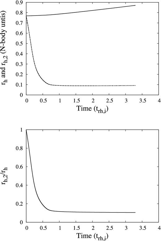
Top: rh (top line) and rh,2 (bottom line) versus time (units trh,i) of gas models with N = 32k, m2/m1 = 10 and M2/M1 = 0.02. rh and rh,2 are given in N-body units. Initially, rh and rh,2 have the same value, but mass segregation quickly decreases rh,2, after which it reaches an approximately steady value. Bottom: rh,2/rh versus time (units trh,i). Core collapse (see Section 2.1) occurs at ≈1trh,i; shortly before this rh,2/rh reaches a nearly constant value.
![The variation of rh,2/rh with m2/m1. The points represent the values of rh,2/rh given in Table 1. The lines represent the expected variation of rh,2/rh with m2/m1 [fitted curves of the form b(m2/m1)0.4] as given by the theory in Section 2.1. The lines have only been included for M2/M1 < 0.1 as this is where the theory is expected to apply. The empirical measured variation of rh,2/rh with m2/m1 is in good agreement with the theory in Section 2.1, when m2/m1 ≳ 10 and M2/M1 < 0.1. See the text for further details.](https://oup.silverchair-cdn.com/oup/backfile/Content_public/Journal/mnras/432/4/10.1093_mnras_stt628/1/m_stt628fig2.jpeg?Expires=1750258261&Signature=OzkYOFj4zLO-XvwYY8TcgFj3KW~5h4fZoJV5CNlyRNAP3p21y6QH-pv90WCurI8nQzxTcL2x1fjW5rTkwLPG3jlp8RnTWtiJwOp3C1vfwpudAoXTH3rJyb3CF8V-sZkzwStT6EHGakOT4OqyX3owd4MBlRWhASznlSVypMKK4z~EfmVza1zpDIwjVJU-LdCLnYJAsLY~v79CfOcNvAT4nQ7hA0iR1UsNh8a8~gUn3duzP-DwA4sLMZKJGxYcqZIjSPX8F~VUBvENTXcaOO7YWA8ljxHwql~vfHbS08ZpN4Rs0pp7JuZFmxzWmeod0B3knHepFSfOOLA9zWDSP2U2XQ__&Key-Pair-Id=APKAIE5G5CRDK6RD3PGA)
The variation of rh,2/rh with m2/m1. The points represent the values of rh,2/rh given in Table 1. The lines represent the expected variation of rh,2/rh with m2/m1 [fitted curves of the form b(m2/m1)0.4] as given by the theory in Section 2.1. The lines have only been included for M2/M1 < 0.1 as this is where the theory is expected to apply. The empirical measured variation of rh,2/rh with m2/m1 is in good agreement with the theory in Section 2.1, when m2/m1 ≳ 10 and M2/M1 < 0.1. See the text for further details.
We now consider the comparison with theory more quantitatively in the regime M2/M1 ≲ 0.1. In Fig. 2 we can see that values of rh,2/rh are also in quantitative agreement with equation (4) for m2/m1 ≳ 10 in the sense that the power-law index is approximately confirmed. However, rh,2/rh increases more rapidly than is expected by equation (4) for m2/m1 < 10 and M2/M1 < 0.05. This behaviour is possibly explained by equation (6), which predicts a different power-law index for Spitzer stable systems from that in equation (4). Indeed, for the lowest values of M2/M1, the slope is approximately consistent with equation (6). Nevertheless, the stellar mass ratios of interest are m2/m1 ≳ 10 as realistic ratios for systems containing BH subsystems would be in this range.
The variation of rh,2/rh with M2/M1 over a range of different N is shown in Fig. 3 for the case m2/m1 = 10. For the case N = 32k, the variation is less than expected from equation (4) (see Section 2.1). The variation is approximately of the same form, i.e. rh,2/rh ∝ (M2/M1)a, but a ≈ 0.3 for the case m2/m1 = 10 and N = 32k, which is less than the expected value of a ≃ 0.6. (Here we ignore the dependence on the Coulomb logarithms.) The variation of rh,2/rh with M2/M1 comes into better agreement with equation (4) with increasing N, with the case N = 128k being in good agreement with the theory in Section 2.1. This seems to indicate that the disagreement is caused by small values of N2. One of the assumptions under which equation (4) is derived is that rc ≪ rh,2, but it is possible that rc,2 ≈ rh,2 for small N2 as shown in equation (5). In this case, one of the assumptions underlying the theory is not satisfied.
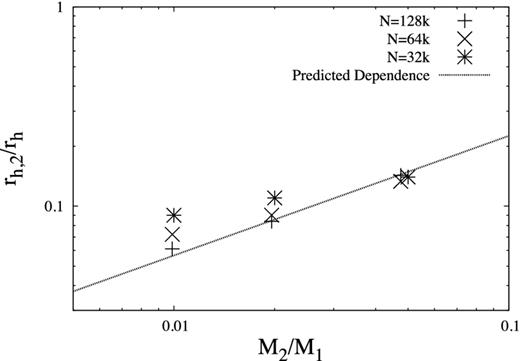
The variation of rh,2/rh with M2/M1. The points represent the values of rh,2/rh for the case m2/m1 = 10 with N = 32k, 64k and 128k. The line represents the expected variation of rh,2/rh with M2/M1 as given by the theory in Section 2.1.
rh,2/rh in N-body runs
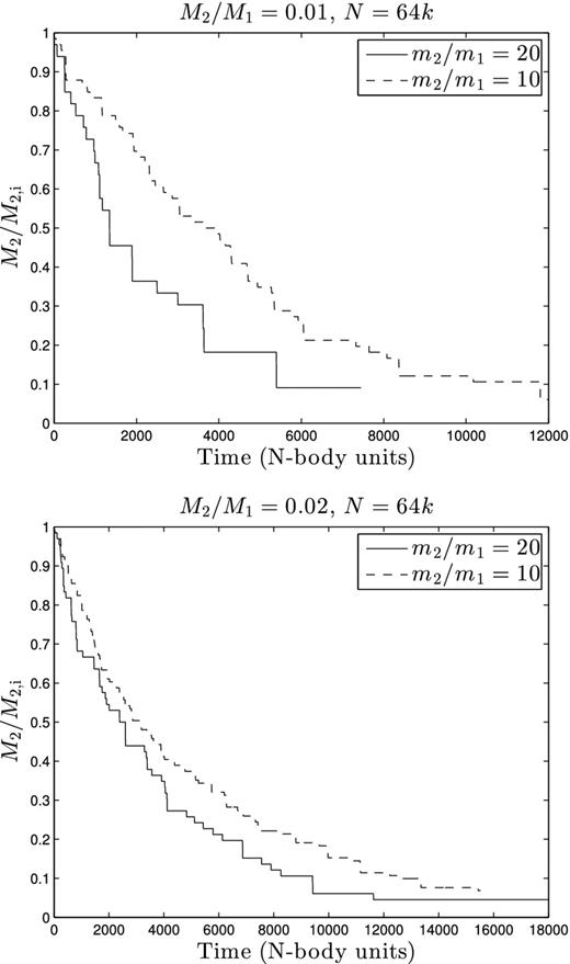
In Section 2.1, it was predicted that rh,2/rh would increase with increasing m2/m1 in a system with fixed M2/M1 and N. This prediction will now be tested with direct N-body runs (see Section 4). The initial conditions are realizations of the Plummer model with N = 64k, M2/M1 = 0.02 and two different values of m2/m1 (10 and 20). We have compared the values of rh,2/rh in Fig. 4. The value of rh,2/rh is indeed larger for m2/m1 = 20 than for m2/m1 = 10 as expected. This effect was confirmed using a two-component gas code in the previous subsection. However, mass is conserved in the gas models, whereas in the more realistic N-body systems mass is lost over time. Therefore, we need to ensure that we compare the values of rh,2/rh for both the runs at constant M2/M1. For the two runs in Fig. 4, mass is lost from the BH subsystem at approximately the same rate (see Fig. 11, bottom), as predicted by the theory in Section 2.5. The mass-loss from the light component is negligible over the length of these N-body runs: less than 5 per cent of the light component is lost during the entire run. Therefore, while M2/M1 does decrease with time over the runs in Fig. 4, the values of M2/M1 for both runs are approximately the same at any given time.
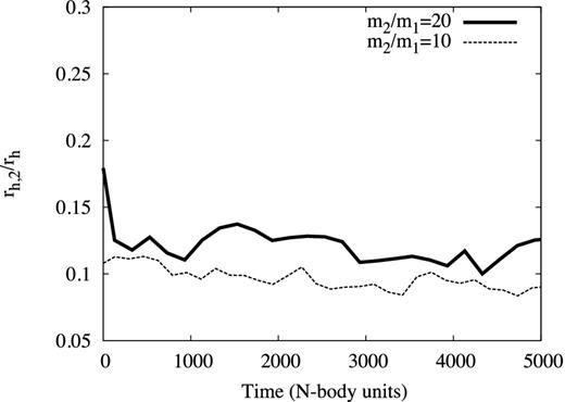
rh,2/rh versus time (in N-body units). N-body runs with initial values N = 64k, M2/M1 = 0.02, m2/m1 = 20 (thick line) and m2/m1 = 10 (thin line). Time is set so that core collapse occurs at t = 0 for both systems. rh,2/rh has been smoothed to make the plot clearer. The values of rh,2/rh in the graph are in approximate agreement with the results from the two-component gas model given in Table 1.
The variation of rh,2/rh with M2/M1 is shown in Fig. 5 for the N-body run with N = 64k, m2/m1 = 10 and M2/M1 = 0.02. Initially, rh,2/rh = 1 before being quickly reduced due to mass segregation. The BH subsystem starts producing energy when rh,2/rh reaches ≈0.1 and M2/M1 begins to decrease at this point. The variation of rh,2/rh with M2/M1 is again less than expected from equation (4), with the result indicating a dependence of rh,2/rh ∝ (M2/M1)0.28. Although this is not in agreement with equation (4) if we neglect the Coulomb logarithm, the results are in good agreement with the gas model.
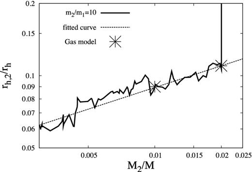
rh,2/rh versus M2/M1. The solid line represents results from an N-body run with initial values N = 64k, M2/M1 = 0.02 and m2/m1 = 10. The results are smoothed to make the value of rh,2/rh clearer. The dotted line denotes the best matching curve of the form b(M2/M1)a (where a and b are constants, the best matching values being b ≈ 0.33 and a ≈ 0.28). The points are results from the two-component gas model (see Table 1), where M2/M1 is fixed. At the beginning of the run, rh,2/rh = 1 before mass segregation rapidly reduces its value, whence the vertical line segment in the top-right corner.
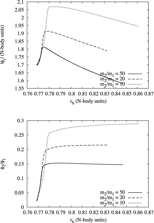
Top: |ϕc| versus rh for gaseous systems with fixed N (128k) and M2/M1 = 0.02; the different values of m2/m1 are 10, 20 and 50. Bottom: ϕ2/ϕ1 versus rh for the same systems as in the top figure. This plot shows that the contribution of the light component to the central potential is dominant.
Central potential
In Section 2.5, we made the assumption that the main contribution to the central potential is from the light component. In order to test this assumption, the central potential and the relative contribution of each component to the central potential (ϕ2/ϕ1) have been measured in a series of two-component gas models with M2/M1 = 0.02. These results are presented in Table 2. The values in Table 2 were measured once the systems had reached a certain value of rh (rh = 0.83). This was done in order to ensure that the systems had reached a similar point in their evolution (see Fig. 6). The variation in ϕc in Table 2 is only about a factor of 1.2 for fixed N even though m2/m1 varies by a factor of 5. The variation in ϕ2/ϕ1 is higher, but the values are of the same order of magnitude as the estimate in Section 2.5 and indeed in satisfactory agreement, considering that M2/M1 is higher here. As the energy generation rate per unit mass is |$\propto m_2^3\rho _2^2/\sigma _2^7$| (Heggie & Hut 2003), for systems with the same value of N, M2/M1 and m1, as m2 increases the system can produce the required energy at a lower central density; thus, the central potential is expected to become shallower with increasing m2/m1 as seen in Table 2. This is also why two-component systems with larger m2/m1 are stable against gravothermal oscillation to higher values of N than for lower m2/m1 (Breen & Heggie 2012a).
Variation of |ϕc| and ϕ2/ϕ1 with m2/m1 for systems with M2/M1 = 0.02. The values are measured in the post-collapse phase of evolution when the systems have reached a certain size (rh ≈ 0.83).
| m2/m1 | N = 32k | N = 128k | ||
|---|---|---|---|---|
| |ϕc| | ϕ2/ϕ1 | |ϕc| | ϕ2/ϕ1 | |
| 50 | 1.55 | 0.10 | 1.62 | 0.15 |
| 20 | 1.67 | 0.14 | 1.80 | 0.22 |
| 10 | 1.85 | 0.18 | 2.00 | 0.28 |
| m2/m1 | N = 32k | N = 128k | ||
|---|---|---|---|---|
| |ϕc| | ϕ2/ϕ1 | |ϕc| | ϕ2/ϕ1 | |
| 50 | 1.55 | 0.10 | 1.62 | 0.15 |
| 20 | 1.67 | 0.14 | 1.80 | 0.22 |
| 10 | 1.85 | 0.18 | 2.00 | 0.28 |
These values serve as a rough guide to how the variation of m2/m1 will affect the system. If we consider systems with fixed N, M2 and M2/M1 and use similar reasoning as in Section 2.5, we would expect systems with lower m2/m1 to last slightly longer than systems with higher m2/m1. This is because the average energy contribution per binary is dependent on the depth of the central potential. The deeper the central potential, the greater the average energy contribution per binary will be, and therefore it is expected that for fixed M2/M1 a two-component system with m2/m1 = 20 will lose mass slightly faster than a system with m2/m1 = 10.
EVOLUTION OF THE BH SUBSYSTEM: DIRECT N-BODY SIMULATIONS
Overview
In order to study BH subsystems, we carried out a number of N-body simulations using the nbody6 code (Nitadori & Aarseth 2012). Because of the computational cost of large N simulations we have mostly limited ourselves to runs with N = 32k and 64k. The total mass ratios used were M2/M1 = 0.01 and 0.02. The stellar mass ratios used were m2/m1 = 10 and 20. An additional run with N = 128k, M2/M1 = 0.02 and m2/m1 = 20 was also carried out to increase the number of systems with N2 > 102. These parameters are summarized in Table 3, and the results of these runs are given in Table 4. A qualitative example of the typical evolution of these systems is given in Fig. 7. The evolution of the fraction of mass remaining in BH (M2/M2, i) in all runs is shown in Figs 10–12.
Parameters used for N-body runs. In all cases the initial conditions were realizations of the Plummer model (Plummer 1911). The values of trh,i (the initial half-mass relaxation time) are calculated using Λ = 0.02N for the Coulomb logarithm.
| N | m2/m1 | M2/M1 | trh,i (N-body units) |
|---|---|---|---|
| 32k | 10, 20 | 0.01, 0.02 | 471 |
| 64k | 10, 20 | 0.01, 0.02 | 851 |
| 128k | 20 | 0.02 | 1552 |
| N | m2/m1 | M2/M1 | trh,i (N-body units) |
|---|---|---|---|
| 32k | 10, 20 | 0.01, 0.02 | 471 |
| 64k | 10, 20 | 0.01, 0.02 | 851 |
| 128k | 20 | 0.02 | 1552 |
Results from N-body runs with parameters given in Table 3. The values given are the stellar mass ratio (m2/m1), initial total mass ratio (M2/M1), initial total particle number (N), initial number of BH (N2), core collapse time (tcc), the time at which 50 per cent (T50 per cent) and 90 per cent (T90 per cent) of the initial BH total mass has escaped, the recollapse time of the system, the rate of mass-loss from the subsystem |$-\skew4\dot{M}_2$|, ζ (see Section 2) and the number of the figure which plots the fraction of remaining BH mass (M2/M2, i) with time. T50 per cent, T90 per cent and the time for recollapse are given in N-body units and given in parentheses in units of trh,i. T50 per cent, T90 per cent and the time for recollapse are measured from the time at which core collapse finishes. The value of T90 per cent for the case m2/m1 = 20, M2/M1 = 0.01 and N = 32k (marked with *) is actually the point where 88 per cent mass-loss occurs; after this point all that remains in the system is a single binary BH. The values of |$\skew4\dot{M}_2$| are given in units of 10−6N-body units (or |$10^{-3}\ t_{\rm rh,i}^{-1}$| for the values in parentheses); these are measured between the loss of the first BH and 50 per cent of the BH, by |$\skew4\dot{M}_2 = -0.5M_{\rm 2,i}/T_{50\,{\rm per\, cent}}$|. The values given in the subscript and superscript are the upper and lower 90 per cent confidence limits assuming that BH escape is a Poisson process. The values of ζ were measured by assuming |$\skew4\dot{E}/|E| \approx \dot{r}_{\rm h}/r_{\rm h}$| (which holds if |E| ∝ GM2/rh and |$\skew4\dot{M}$| is small) and evaluating |$\small { \frac{0.138N}{\ln {\Lambda }} \frac{2}{3}\frac{d(r_{\rm h}^{\frac{3}{2}})}{dt} (\approx t_{\rm rh}\frac{\dot{r}_{\rm h}}{r_{\rm h}}}$|N-body units) between 2tcc and tcc + T50 per cent. |$\small {\frac{\text{d}(r_{\rm h}^{\frac{3}{2}})}{\text{d}t}}$| was evaluated by taking the slope of the best-fitting line to |$r_{\rm h}^{\frac{3}{2}}$|; the typical errors with the fitted lines were small, <3 per cent.
| |$\frac{m_{2}}{m_1}$| | |$\frac{M_{2}}{M_1}$| | N | N2 | tcc | T50 per cent a | T90 per cent a | Recollapse timea | |$-\skew4\dot{M}_2\,^b$| | ζ | Figures |
|---|---|---|---|---|---|---|---|---|---|---|
| 10 | 0.01 | 32k | 34 | 530 | 2070 (4.4) | 5610 (11.9) | 8748 (18.6) | |$2.4^{3.6}_{1.5}$| (|$1.1^{1.7}_{0.7}$|) | 0.03 | 10 (top) |
| 20 | 0.01 | 32k | 17 | 380 | 850 (1.8) | 3000* (6.3*) | >8000 (17.0) | |$5.9^{10.6}_{2.9}$| (|$2.8^{5.0}_{1.4}$|) | 0.06 | 10 (top) |
| 10 | 0.02 | 32k | 66 | 492 | 1658 (3.5) | 5702 (12.1) | >11 876 (25.2) | |$6.0^{8.1}_{4.4}$| (|$2.8^{3.8}_{2.1}$|) | 0.06 | 10 (bottom) |
| 20 | 0.02 | 32k | 33 | 419 | 940 (1.9) | 3816 (8.1) | >9902 (21.0) | |$10.6^{16.0}_{6.8}$| (|$5.0^{7.5}_{3.2}$|) | 0.10 | 10 (bottom) |
| 10 | 0.01 | 64k | 66 | 920 | 3650 (4.2) | 12 950 (15.2) | >13 000 (15.3) | |$1.4^{1.8}_{1.0}$| (|$1.2^{1.6}_{0.9}$|) | 0.03 | 11 (top) |
| 20 | 0.01 | 64k | 33 | 404 | 1750 (2.1) | 5400 (6.8) | >7844 (9.2) | |$2.9^{4.3}_{1.8}$| (|$2.4^{3.6}_{1.5}$|) | 0.05 | 11 (top) |
| 10 | 0.02 | 64k | 131 | 690 | 3230 (3.7) | 12 740 (14.6) | >15 580 (17.9) | |$3.5^{4.3}_{2.9}$| (|$2.6^{3.2}_{2.1}$|) | 0.05 | 11 (bottom) |
| 20 | 0.02 | 64k | 66 | 270 | 2680 (3.2) | 9495 (11.3) | >19 600 (23.4) | |$3.7^{5.0}_{2.7}$| (|$3.2^{4.2}_{2.3}$|) | 0.08 | 11 (bottom) |
| 20 | 0.02 | 128k | 131 | 650 | 4120 (2.7) | >7076 (4.6) | >7076 (4.6) | |$2.4^{3.0}_{2.0}$| (|$3.8^{4.6}_{3.0}$|) | 0.08 | 12 |
aUnits: N-body units (trh,i).
bUnits: 10−6N-body units (|$10^{-3}\ t_{\rm rh,i}^{-1}$|).
First we will discuss the qualitative behaviour of systems containing a BH subsystem. We do this by considering the case m2/m1 = 20, M2/M1 = 0.02 and N = 64k, which we refer to henceforth as (20, 0.02, 64k). The graphs of rh and rc against time for this run are shown in Fig. 7. The BH population quickly segregates to the centre of the system causing core collapse to occur in the BH subsystem. For the parameters of this model, this takes approximately 0.3trh,i (where trh,i is the initial half-mass relaxation time) to occur. The collapse time for other parameter choices is discussed at length in Breen & Heggie (2012a). In Fig. 7, this occurs at 270 N-body units. We will refer to this as the first collapse. This is followed by a phase of powered expansion. This can be seen in Fig. 7 where, after the first collapse, both rc and rh increase up until ∼5000 N-body units. As BH escape, the BH subsystem becomes less efficient at producing energy (see Section 2.3) and the rate of expansion decreases. The core stops expanding and begins to contract again at ≈7500 N-body units; at this stage there is only 15 per cent of the BH subsystem remaining (see Fig. 11, bottom, solid line). Most of the remaining BH escape before ≈9500 N-body units leaving the system with a single remaining BH binary from ∼11 500 N-body units. The contraction of the core that begins after ≈7500 N-body units shall be referred to as the second core collapse or recollapse. As with the first core collapse the core contracts because there is not enough energy being produced to meet the energy demands of the cluster. As the core (which is dominated by the low-mass stars as most of the BH have escaped) becomes smaller towards the end of the run, the remaining BH binary starts to interact strongly with the light stars, producing energy more efficiently. This causes the more rapid increase in rh seen towards the end of the plot. The contraction of the core was still ongoing at the end of the run. The core will presumably continue to contract until balanced evolution is restored. If the last remaining BH binary is providing most of the energy, then how long that binary persists in the system depends on the hardness of that binary. Assuming that the last BH binary is only slightly hard, it is possible that the core contracts sufficiently for a single BH binary to produce the required energy to power the expansion of the system. Ultimately the BH binary will become hard enough to cause its ejection from the system. However, if it is extremely hard, it is likely that the binary gets ejected from the system during the second core collapse. If this happens, the collapse of the core will continue until light binaries are produced as in a one-component model.
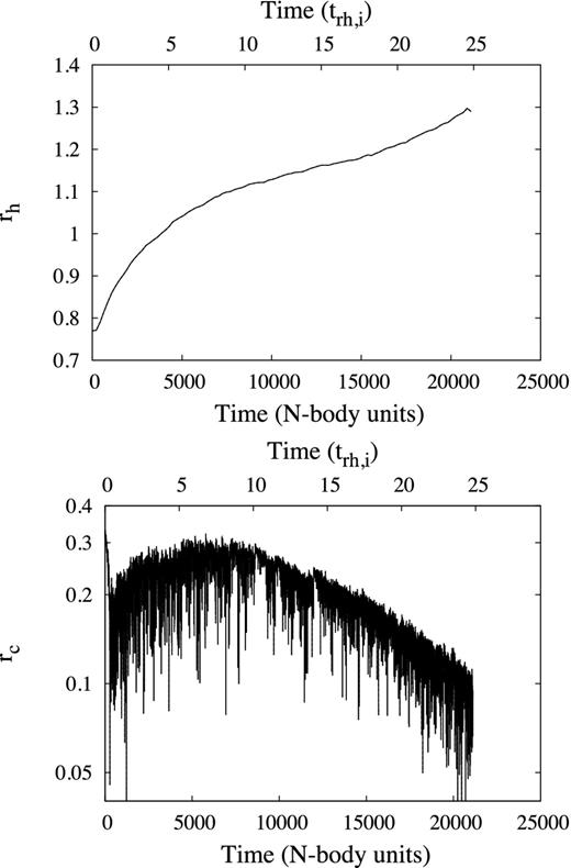
N-body run (20, 0.02, 64k), i.e. with N = 64k, m2/m1 = 20 and M2/M1 = 0.02. Bottom: rc versus time (N-body units). At t = 270, N-body units core collapse occurs. After most of the BH have escaped (t ≈ 7500), the core starts to recollapse. Top: rh versus time (N-body units). rh initially expands rapidly before gradually slowing down as the BH subsystem dissolves. From t ≈ 10 000 to ≈15 000 there is little change in rh as the system is no longer in a balanced energy generating phase of evolution. The expansion after t ≈ 15 000 results from a single remaining BH binary which becomes more active as the core collapses.
The rate of loss of BH
Now we compare the values of |$\skew4\dot{M}_2$| with the theory of Section 2.5 (equation 10). |$\skew4\dot{M}_2$| is estimated by calculating the average mass-loss rate over the time taken (from the start of mass-loss) for the BH subsystem to lose 50 per cent of its initial mass (i.e. 0.5M2, i/T50 per cent, where T50 per cent is the time taken from tcc until 50 per cent of the BH subsystem has escaped; see Table 4 for details). Note that there is a small systematic error introduced by measuring mass-loss from the point at which it first occurs. The values of |$\skew4\dot{M}_2$| (in units of |$10^{-3}t_{\rm rh,i}^{-1}$|) are plotted in Fig. 8. The error bars (estimated as stated in the caption of Table 4) are large because N2 is relatively small, and most data points are consistent with a value of approximately |$3\times 10^{-3}t^{-1}_{\rm rh,i}$|. Equation (10) with canonical values of α, β and ζ implies that the values in Fig. 8 should be nearly |$6.1 \times 10^{-3}t^{-1}_{\rm rh,i}$|, and we will now consider reasons for the discrepancy.
![$\skew4\dot{M}_2$ (units of $10^{-3}t_{\rm rh,i}^{-1}$) versus initial value of N2. The error bars indicate confidence limits (see Table 4 for details). The circles represent (20, M2/M1, N), squares represent (10, M2/M1, N), filled symbols represent (m2/m1, 0.02, N), unfilled symbols represent (m2/m1, 0.01, N), larger symbols (m2/m1, M2/M1, 64k) [with the exception of the largest circle on the right which corresponds to (20, 0.02, 128k)] and smaller symbols (m2/m1, M2/M1, 32k). For cases with the same or similar initial values of N2, some of the values were adjusted by ≲10 per cent to stop the symbols from overlapping. To a first approximation, $\skew4\dot{M}_2$ is independent of m2/m1, M2/M1 and N.](https://oup.silverchair-cdn.com/oup/backfile/Content_public/Journal/mnras/432/4/10.1093_mnras_stt628/1/m_stt628fig8.jpeg?Expires=1750258261&Signature=f7qFEejBf4zVsbx-jNkfXLGnIx5D8xvj7-MtE1U5~trztM4OZ7WO7qVj8rwNQNrdvOQLdtz-MEIELARh7Mb-if44CTv-FpSnMViPuwQJR8yfGX6Wo0bOm5BZam9qh7ncl6r-pIBjpA79qxpOsJCGRNmapLHTD8J7vF-NqjHWHJJ3rIO6khF4beXhMRMQDsYjRWJaZTw~cjMhYNTbVU2PXKiMwjedl-b9n40Nuu2WmpU6gy5SMGbJUJWdfDFq3bHLMEHAjCtbARKfabF~aJQH3ScxluA-IRZ6BZkAyRMoEKn8Ma8dqqGGiTfK7DjEv2ijeBUkbqR5dCK90wHDBMcg9w__&Key-Pair-Id=APKAIE5G5CRDK6RD3PGA)
|$\skew4\dot{M}_2$| (units of |$10^{-3}t_{\rm rh,i}^{-1}$|) versus initial value of N2. The error bars indicate confidence limits (see Table 4 for details). The circles represent (20, M2/M1, N), squares represent (10, M2/M1, N), filled symbols represent (m2/m1, 0.02, N), unfilled symbols represent (m2/m1, 0.01, N), larger symbols (m2/m1, M2/M1, 64k) [with the exception of the largest circle on the right which corresponds to (20, 0.02, 128k)] and smaller symbols (m2/m1, M2/M1, 32k). For cases with the same or similar initial values of N2, some of the values were adjusted by ≲10 per cent to stop the symbols from overlapping. To a first approximation, |$\skew4\dot{M}_2$| is independent of m2/m1, M2/M1 and N.
First, this estimate can be improved upon by taking into account the fact that the system expands as energy is being generated, increasing the relaxation time and in turn decreasing the mass-loss rate. The improved estimate can be calculated by using equation (12) to estimate the time taken for half the BH to be lost and evaluating |$\skew4\dot{M}_2$| as was done in Table 4. This results in a slightly smaller estimate of |$5.4\times 10^{-3}t^{-1}_{\rm rh,i}$|, which is still significantly larger than most of the values in Table 4.
Another factor is that the values of ζ for most of the runs are smaller than the canonical value used for the estimate (i.e. ζ ≈ 0.09). Equation (12) predicts an approximately linear dependence of |$\skew4\dot{M}_2$| on ζ, and this is clearly confirmed in Fig. 9. The solid line, which represents the predicted values of |$\skew4\dot{M}_2$| with varying ζ, nevertheless lies above all the numerical results and outside the confidence intervals for all but a few of the runs. However, by adjusting the value of α/β (in equations 10 and 12 α and β only appear in the form α/β) from α/β ≈ 0.068 (the value estimated on the basis of theoretical arguments) to α/β ≈ 0.051, the theory comes into very good agreement with the values of |$\skew4\dot{M}_2$|. This can be seen in Fig. 9 where the dashed line represents the predicted values of |$\skew4\dot{M}_2$| based on a value of α/β ≈ 0.051. The discussion of Section 2.5 makes it clear that the canonical values of α and, especially, β are subject to uncertainty, the latter resting entirely on approximate theoretical arguments. The suggested revision of α/β cannot be ruled out on these grounds.
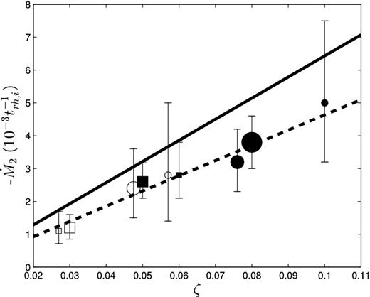
|$\skew4\dot{M}_2$| (units of |$10^{-3}t_{\rm rh,i}^{-1}$|) versus value of ζ; the error bars indicate 90 per cent confidence limits (see Table 4 for details). The symbols represent the same runs as in Fig. 8, the solid line represents the predicted values of |$\skew4\dot{M}_2$| using the value of α/β = 0.068 (based on theoretical arguments) and the dashed line represents the predicted values of |$\skew4\dot{M}_2$| using the value of α/β = 0.051 (the empirical value). For cases with the same or similar values of ζ, some of the values of ζ were adjusted by ±5 per cent to stop the symbols from overlapping. See the text for details.
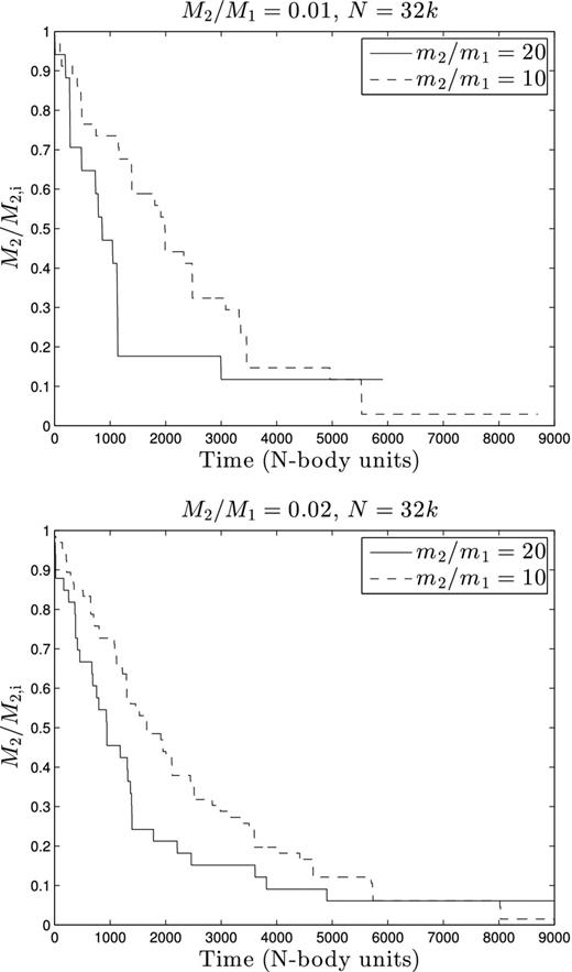
Fraction of initial mass remaining (M2/M2, i, where M2, i is the initial mass of the heavy component) versus time (in N-body units) for the cases N = 32k with M2/M1 = 0.01 (top) and M2/M1 = 0.02 (bottom). In both figures the dashed line represents m2/m1 = 10 and the solid line represents m2/m1 = 20. T = 0 is set as the time when first mass-loss occurs, which is at approximately the same time as the first core collapse.
Equation (13) allows us to test the theory constructed in Section 2.5, in a ζ-independent way. In Fig. 13 the observed dependence of M2 on rh is in satisfactory agreement with the predictions based on equation (13).
Fraction of initial mass remaining (M2/M2, i, where M2, i is the initial mass of the heavy component) versus time (in N-body units) for the cases N = 64k with M2/M1 = 0.01 (top) and M2/M1 = 0.02 (bottom). In both figures the dashed line represents m2/m1 = 10 and the solid line represents m2/m1 = 20. T = 0 is set as the time when the first mass-loss occurs, which is at approximately the same time as the first core collapse.
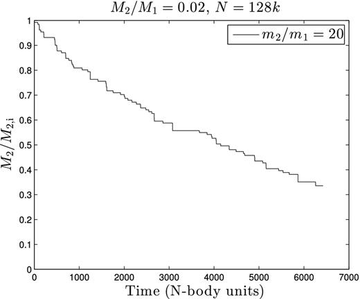
Fraction of initial mass remaining (M2/M2, i, where M2, i is the initial mass of the heavy component) versus time (in N-body units) for the case N = 128k with M2/M1 = 0.02 and m2/m1 = 20. T = 0 is set as the time when the first mass-loss occurs, which is at approximately the same time as the first core collapse.
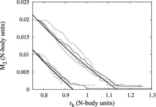
Evolution of M2 versus rh for the N = 32k and 64k models in Table 4. The thick dashed line shows the theoretical prediction (see equation 13) for the initial value of M2/M1 = 0.02 and the thick solid line shows the theoretical prediction for the initial value of M2/M1 = 0.01. The value of rh,i used in equation (13) was 0.77 and the empirical value of α/β ≈ 0.051 was used for all models. In all cases, the behaviour of the N-body runs is in approximate quantitative agreement with the predicted behaviour until there are only a few BH remaining.
The lower values of ζ in Table 4 may result from systems in which the BH subsystem is incapable of producing the required energy for the system to achieve balanced evolution. This could possibly be due to the small values of N2; most of these models reach values of N2 (at time T50 per cent) below the point at which the theory of Section 2.5 is expected to apply (see Section 2.3). If a system is not in balanced evolution, it is expected to undergo contraction of the inner Lagrangian radii relative to rh, qualitatively as in conventional core collapse. This is illustrated in Fig. 14 for three of the N-body runs in Table 4. The systems with smaller values of ζ show greater contraction. Note that the values ζ are only evaluated over the period to T50 per cent and appear to decrease after T50 per cent (∼3000). Indeed, this is what would be expected as the expansion is affected by the weakening energy generation (see also Fig. 7).
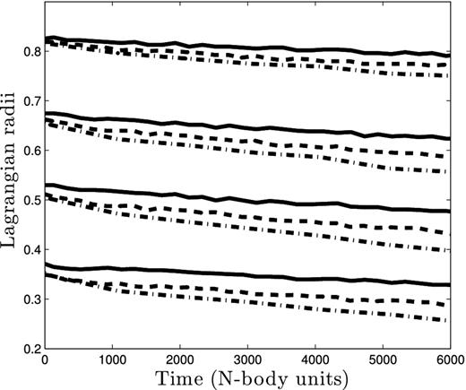
Relative contraction in Lagrangian radii (40, 30, 20 and 10 per cent) over time (N-body units) for (20, 0.02, 64k; solid line), (10, 0.02, 64k; dashed line) and (10, 0.01, 64k; dot–dashed line). T = 0 in all models is set as the time mass-loss starts from the BH subsystem. Radii are measured in units of the half-mass radius. The values of ζ for the three runs are 0.08, 0.05 and 0.03, respectively. The parameter ζ measures the dimensionless expansion rate of the half-mass radius, and slow expansion is associated with relative contraction of the inner Lagrangian radii.
In this section we have assumed that mass segregation concentrates the BH in the centre of the system by the time of the first core collapse. Though this prevents further contraction of the central BH subsystem, this is not true of all the BH, as discussed in Appendix B and Morscher et al. (2012). The outermost BH can continue contracting after core collapse has occurred, indicating that mass segregation can continue in the outermost parts of a system for a while after core collapse. This results in additional heating which is not associated with energy production. The effect of this heating is expected to be small for the models in Table 3 due to the small particle number, although the effect may be more significant in larger systems and may be enhanced by the presence of a mass spectrum.
Lifetime of BH subsystems
Now that the dependence of |$\skew4\dot{M}_2$| on cluster properties has been discussed, it is natural to move on to considering how long the BH subsystem lasts. For this purpose we shall define the lifetime of the BH subsystem as the time taken from the core collapse of the BH subsystem (which occurs at tcc) until the BH subsystem has lost 90 per cent of its initial mass (T90 per cent). These values are given in Table 4, where it can be seen that T90 per cent ∼ 10trh,i. Equation (12) in Section 2.5 can be used to estimate the lifetime of the subsystem (using α/β = 0.051). For M2/M1 = 0.01, the theory predicts T90 per cent ∼ 2.2trh,i and ∼5.2trh,i for M2/M1 = 0.02. These values are significantly smaller than the values seen in Table 4. As stated in the previous subsection, most of the values of ζ in Table 4 are below the value used in Section 2.5. Adjusting ζ to 0.05 in equation (12) increases the predicted values of T90 per cent to 4.0trh,i for M2/M1 = 0.01 and 9.3trh,i for M2/M1 = 0.02. These values are still significantly smaller than those given in Table 4 with the corresponding value of ζ. The difference between the empirically found values and the theoretical estimates might be accounted for by the fact that the theory assumes a constant value of ζ; however, ζ is expected to decrease as the BH subsystem evaporates (see Section 4.1). This behaviour is illustrated by the behaviour of rh in Fig. 7. There is a hint that the same decrease of ζ with decreasing N may also be present in one-component models (Alexander & Gieles 2012). Also as can be seen from the values of ζ in Table 4, some systems appear to be incapable of achieving balanced evolution at any time throughout the loss of the BH subsystem.
The expected evolution of a BH subsystem can be illustrated using Fig. 9. If we assume that the BH subsystem is capable of achieving balanced evolution, after the formation of the BH subsystem ζ and |$-\skew4\dot{M}_2$| are predicted to rapidly reach the balanced evolution values of ζ ≈ 0.09 and |$-\skew4\dot{M}_2\approx 4 \times 10^{-3}t^{-1}_{\rm rh,i}$| (just to the upper right of the large filled circle). As the BH subsystem loses mass, it will eventually reach the point where it is no longer capable of generating the energy needed for balanced evolution. After this, the system will move down the dashed line towards the origin. As it does so, the rate of mass-loss decreases, prolonging the life of the BH subsystem. This picture may explain the longer lifetimes given in Table 4 and is consistent with the evolution of rh in Fig. 7.
Finally, we briefly consider the recollapse time of these systems (see Table 4). This is the time between the first and second core collapse. It can be interpreted as approximately the time it takes for the system to achieve balanced evolution once the BH subsystem has been exhausted. Most of the N-body runs do not reach the second core collapse, and therefore mostly lower limits on the recollapse time are given in Table 4. From the results in Table 4, this time is at least roughly the same time as the core collapse time of a one-component Plummer model (≈15trh,i; see Heggie & Hut 2003) but can be longer because of the offsetting effect of BH heating.
GRAVOTHERMAL OSCILLATIONS
The conditions for the onset of gravothermal oscillations in two-component models have been studied by Breen & Heggie (2012a), who found that the value of N2 (the number of heavy stars) could be used as an approximate stability condition (where the stability boundary is at N2 ∼ 3000) for a wide range of stellar and total mass ratios (2 ≤ m2/m1 ≤ 50 and 0.1 ≤ M2/M1 ≤ 1.0). Breen & Heggie (2012b), who researched the onset of gravothermal oscillation in multicomponent systems, found that the parameter called the effective particle number Nef (defined as M/mmax) could be used as an approximate stability condition for both the multicomponent systems they studied and the two-component models of Breen & Heggie (2012a). The stability boundary they found was at Nef ∼ 104, which is also consistent with the stability boundary of the one-component model at N = 7000 (Goodman 1987). However, both those stability conditions relied on the assumption that the heavy component (or heavier stars for the multicomponent case) dominated the evolution of the system, in the sense that the heavy component determined the rate of energy generation. This is not the case for the systems considered in this paper as the total mass in the heavy component is so small, and so Nef will not be considered further. (In the systems considered in this paper, the heavy component dominates the production of energy, but the light component controls how much energy is created.) We will now investigate the onset of gravothermal oscillation for the systems of interest in this paper (where M2/M1 ≪ 1.0 and m2/m1 ≳ 5).
The critical number of stars (Ncrit) at which gravothermal oscillations first manifest was found for the gas models with |$M_2/M_1=0.05\text{ and }0.01$|, and m2/m1 = 5, 10, 20 and 50 (see Section 3). The results are given in Table 5. The values of N2 at Ncrit for the runs in Table 5 are given in Table 6. The values for M2/M1 = 0.5 and 0.1 from Breen & Heggie (2012a) have also been included in Tables 5 and 6 for reference. For fixed m2/m1, the system becomes unstable at a roughly fixed value of N2 (N2 ≈ 1500 for M2/M1 = 0.05 and N2 ≈ 900 for M2/M1 = 0.01). These results suggest that N2 still provides an approximate stability condition (for fixed M2/M1) even for models in which the heavy component only makes up a tiny fraction of the system.
Critical values of N in units of 104.
| |$\frac{m_{2}}{m_1}\backslash \frac{M_2}{M_1}$| | 0.5 | 0.1 | 0.05 | 0.01 |
|---|---|---|---|---|
| 50 | 30 | 100 | 130 | 450 |
| 20 | 13 | 36 | 63 | 180 |
| 10 | 7.2 | 22 | 32 | 90 |
| 5 | 4.0 | 10 | 17 | 40 |
| |$\frac{m_{2}}{m_1}\backslash \frac{M_2}{M_1}$| | 0.5 | 0.1 | 0.05 | 0.01 |
|---|---|---|---|---|
| 50 | 30 | 100 | 130 | 450 |
| 20 | 13 | 36 | 63 | 180 |
| 10 | 7.2 | 22 | 32 | 90 |
| 5 | 4.0 | 10 | 17 | 40 |
Values of N2 at Ncrit in units of 103.
| |$\frac{m_{2}}{m_1}\backslash \frac{M_2}{M_1}$| | 0.5 | 0.1 | 0.05 | 0.01 |
|---|---|---|---|---|
| 50 | 3.0 | 2.0 | 1.3 | 0.9 |
| 20 | 3.2 | 1.8 | 1.6 | 0.9 |
| 10 | 3.4 | 2.2 | 1.6 | 0.9 |
| 5 | 3.6 | 2.0 | 1.7 | 0.8 |
| |$\frac{m_{2}}{m_1}\backslash \frac{M_2}{M_1}$| | 0.5 | 0.1 | 0.05 | 0.01 |
|---|---|---|---|---|
| 50 | 3.0 | 2.0 | 1.3 | 0.9 |
| 20 | 3.2 | 1.8 | 1.6 | 0.9 |
| 10 | 3.4 | 2.2 | 1.6 | 0.9 |
| 5 | 3.6 | 2.0 | 1.7 | 0.8 |
Given that the theory in this paper is built around the assumption that the light component determines the evolution of the BH subsystem, it may be surprising that the appearance of gravothermal oscillations seems solely determined (for fixed M2/M1) by the number of stars in the heavy component. However, this may be explained if one considers the unique structure of systems containing a BH subsystem. The presence of a BH subsystem tends to produce a system with two cores, one small BH core and another much larger light core, which is larger than the half-mass radius of the BH subsystem (Merritt et al. 2004; Mackey et al. 2008; also see Fig. 15 in this paper). As gravothermal oscillation in a one-component system requires a small core to half-mass ratio (Goodman 1987), the light system itself is expected to be highly stable against gravothermal oscillations. However, as the BH subsystem has to meet the energy generation requirements of the entire system, the BH subsystem can have a very small ratio of core radius to half-mass radius (see Section 2). If the onset of gravothermal oscillation is a result of the BH subsystem itself becoming unstable, then it would be expected that the BH subsystems would have a similar structure at the stability boundary. This is indeed the case as can be seen in Fig. 15 which shows the post-collapse density profile of two systems (with m2/m1 = 50 and 10) near the stability boundary (i.e. N is slightly smaller than Ncrit): the profiles of the heavy component are almost identical (in terms of density contrast, i.e. ρ2/ρh,2), whereas the profiles of the light component are significantly different. In fact, if one were to plot the BH subsystems in units of ρc,2 versus rc,2, the BH subsystems would be nearly indistinguishable. We study this more quantitatively below.
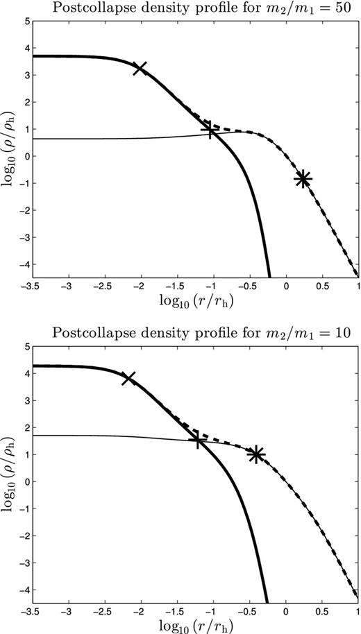
Post-collapse density profile in gas models of two-component systems with M2/M1 = 0.01 near the onset of gravothermal oscillations for m2/m1 = 50 (N = 4.3 × 10⁶, top) and m2/m1 = 10 (N = 8.5 × 10⁵, bottom). The following is shown in the plot: ρ1 (thin line), ρ2 (thick line), ρtot (dashed line), core radius of heavy component rc,2 (×), core radius of light component rc,1 (*) and rh,2 (+). The core radii have been defined as |$r_{{\rm c},i}=\sqrt{9\sigma _{{\rm c},i}^2/(4\pi \rho _{{\rm c},i})}$|. For the case m2/m1 = 50, the BH subsystem creates a density hole in the light component: the density of lights in the centre is approximately a factor of 2 less than its highest value (which occurs at log r/rh ≃ −0.5). The remarkably large value of rc,1 for this case results from the low value of ρc,1 and a high value of |$\sigma _{\rm c,1}^2$| caused by the presence of the BH subsystem.
Values of log10ϵBH and rc,2/rh,2 near Ncrit for systems with M2/M1 = 0.01. For the corresponding values of Ncrit see Table 5. The results in this table indicate that gravothermal oscillation manifests once a certain value of rc,2/rh,2 (or log10ϵ) is reached. See the text for details.
| m2/m1 | 5 | 10 | 20 | 50 |
| rc,2/rh,2 | 0.14 | 0.12 | 0.12 | 0.11 |
| log10ϵBH | −0.21 | −0.30 | −0.31 | −0.32 |
| m2/m1 | 5 | 10 | 20 | 50 |
| rc,2/rh,2 | 0.14 | 0.12 | 0.12 | 0.11 |
| log10ϵBH | −0.21 | −0.30 | −0.31 | −0.32 |
The critical values of log10ϵBH are larger than the values of log10ϵ found for two-component models by Kim et al. (1998) and Breen & Heggie (2012a), and that found for the one-component model by Goodman (1993) by approximately 1.7 dex. Also the critical values of rc,2/rh,2 are larger than the corresponding critical value for a single-component system (Goodman 1987), i.e. rc/rh ≈ 0.02. This may be because the maximum radius of the isothermal region in the BH subsystem is larger than rh,2, as was hinted by Breen & Heggie (2012a). If the condition for gravothermal instability is that the density contrast across the isothermal region exceeds some critical value, and if the edge of this region is well outside rh,2, then it can be understood why the critical value of rc,2/rh,2 is larger than Goodman's value. To investigate this, the size of the isothermal region was measured for (50, 0.01, 4.3 × 10⁶), which is shown in Fig. 15 (top). The edge of the isothermal region (riso) was defined as the radius at which |$\sigma _2^2$| reaches 80 per cent of its central value. This gives rc,2/riso ≈ 0.022 which is consistent with the value of rc/rh found by Goodman (1987) for the one-component model. (For a one-component gas model, rc/riso ≃ 0.016 near the stability boundary.)
CONCLUSION AND DISCUSSION
Summary
In this paper we have studied systems intended to resemble those containing a significant population of BH, i.e. two-component systems with one component being the BH and the other the rest of the stars in the system. It was argued in Section 2.4 that mass-loss by evaporation due to two-body relaxation in the BH subsystem does not cause significant mass-loss of BH and can be neglected. The principal mechanism for removing BH, for the models considered in this paper, is superelastic encounters involving BH binaries and a single BH in the core of the BH subsystem. By considering these systems to be in balanced evolution, predictions were made regarding the BH subsystem, for example the escape rate of BH (see Section 2.5). Some of the potential limitations of the theory were also discussed in Section 2.3.
The theory in Sections 2.1 and 2.2 makes predictions about the structure of the BH subsystem, particularly regarding the variation of rc,2/rh,2 with m2/m1 and M2/M1 (see equation 5). (Here the subscripts 2 and 1 refer to the BH and the other stars, M and m denote the total and individual masses, and rc and rh denote the core and half-mass radii, respectively.) The theory was tested in Section 3.1 with gas models and was found to be in good agreement with theory under the condition that m2/m1 ≳ 10 and that N ≳ 128k (see Figs 2 and 3). The disagreement with the theory outside of those conditions may be attributable to small N2 and the fact that the systems become Spitzer stable at low m2/m1. One of the assumptions of the theory was that the BH subsystem only made a small contribution to the central potential (see Section 2.5), which was tested in Section 3.3 by measuring the contribution to the central potential of each component in a series of simulations.
It was argued in Section 2.5 that the rate of mass-loss from the BH subsystem should be approximately independent of the properties of the BH subsystem (i.e. M2/M1 and m2/m1). This theory only requires that the light component regulates the rate of energy production and does not rely on the stronger assumption that energy is transported through the BH subsystem as outlined in Section 2.1. In Section 4.2 the results of a number of N-body runs were presented (see Tables 3 and 4), and the results were used to test the predicted mass-loss rates from Section 2.5. With the exception of systems with m2/m1 = 10 and M2/M1 = 0.01, the mass-loss rates for the BH subsystem were all consistent with a value of |$\skew4\dot{M}_2 \sim 3.0\times 10^{-3}t_{\rm rh}^{-1}$|, where trh is the half-mass relaxation time of the entire system. However, most of the runs had a lower value of the dimensionless expansion rate ζ than expected and |$\skew4\dot{M}_2$| was found to vary approximately linearly with ζ (see Fig. 9). Once the variation of ζ was taken into account and the value of α/β (where α and β are dimensionless parameters determining the energy and central potential) was adjusted to 0.051 (see Sections 2.5 and 4.2), there was good agreement between the empirical values of |$\skew4\dot{M}_2$| in Table 4 and the predicted values of |$\skew4\dot{M}_2$| made using equation (12). The low values of ζ seen in Table 4 may result from the small number of BH in these systems which possibly results in the inability of the BH subsystem to maintain balanced evolution. Larger simulations will be required before this explanation can be confirmed.
In Section 5 we considered gravothermal oscillations in systems containing a BH subsystem. This extends the parameter space of two-component clusters studied by Breen & Heggie (2012a) to lower values of M2/M1 for m2/m1 ≥ 5. The results in this section imply that the gravothermal instability manifests when the BH subsystem reaches a certain profile (see Fig. 15 and Table 7). A version of the Goodman stability parameter was also tested for systems with M2/M1 = 0.01 and was found to provide an approximate stability condition, although the critical value was significantly larger than the value measured for one-component models. The difference between the critical values for the BH subsystems and the one-component models may result from the fact that the BH subsystem is approximately isothermal to larger radii than rh,2. The ratio between rc,2 and the radius of the isothermal region (riso) was measured for a selected model and was found to be consistent with the critical value of rc/riso found for a one-component system. These results indicate that the onset of gravothermal oscillation for systems containing a BH subsystem is determined by the properties of the BH subsystem.
Astrophysical issues
In this paper we have made several simplifying assumptions. Importantly, we have ignored stellar evolution and the effect of a mass spectrum. A mass spectrum can increase the rate of evolution of a system (Gieles et al. 2010), which by the theory in Section 2.5 would lead to a faster escape rate of BH. On the other hand, mass-loss via stellar evolution from the formation of the BH can cause the system to expand (Mackey et al. 2008), increasing the relaxation time in the system. This in turn would reduce the rate of energy generation in the system, which by the theory in Section 2.5 would prolong the life of the BH subsystem.
Another simplifying assumption was not to consider the removal of BH by natal kicks, which if large could significantly reduce the retained BH population. The topic of natal kicks for BH is still under debate, so here we will only give the topic very general consideration. The ejection of BH by natal kicks is itself an energy source, which heats the system in qualitatively the same way as a BH ejected by superelastic encounters with binaries. Also if a natal kick is not significant enough to remove a BH from the system, the BH would shed much of the kinetic energy gained from the kick to the other stars in the system. This is analogous to the results of Fregeau et al. (2009), who found that adding natal kicks to white dwarfs was an additional energy source.
Another topic we have ignored is the presence of more than one stellar population in many globular clusters. In the typical scenario for the formation of the second generation stars in a globular cluster (Ventura et al. 2001), ejecta from asymptotic giant branch stars cools and collects in the centre of the cluster. If a BH subsystem is already present at the centre, this could lead to a significant increase in the stellar mass of the BH (Krause et al. 2012; Leigh et al. 2012) and by the theory in Section 2 an increase in the total mass of the BH subsystem would increase its lifetime. Even in a single population scenario, physical collisions can occur between BH and other stars in the system (Giersz et al. 2012), and this would also increase the total mass in the BH subsystem.
We have not considered systems which contain an intermediate mass black hole (IMBH) alongside a BH subsystem. A recent radio survey by Strader et al. (2012) found no evidence of IMBH in the three globular clusters M15, M19 and M22. However, there could be other clusters which contain both an IMBH and a BH subsystem, and this would be an interesting topic for future work.
Classification of two-component systems
In Section 5 we considered gravothermal oscillations in systems containing a BH subsystem. This extends the parameter space of two-component clusters studied by Breen & Heggie (2012a) to lower values of M2/M1 for m2/m1 ≥ 5. But there are rather distinct physical characteristics of the systems studied in the two papers, as we have already seen in the study of gravothermal oscillations (Section 5). Here we attempt to summarize these ideas.
In order to differentiate between two-component systems, a classification scheme has been devised that divides the two-component system parameter space into four regions (see Fig. 16). The criteria used to divide the parameter space are (a) whether or not the isothermal region which becomes gravothermally unstable is associated with the heavy component (regions II and III) or the light component (regions I and IV), (b) whether or not the system is Spitzer stable (region I) or Spitzer unstable (regions II and III) and (c) whether or not the two-body relaxation process within rh is dominated by the heavy component (region II) or the light component (regions I, III and IV). The differences between the regions are summarized in Table 8. We shall now justify the classification by considering each of the criteria used more closely.
Summary of the different regions in the parameter space of two-component systems. The table states whether a given dynamical process is dominated by the light or heavy component of the system. trh represents the two-body relaxation time within rh, trc represents the two-body relaxation time within rc, GTO stands for gravothermal oscillations, with reference to which component contains the large isothermal region which becomes unstable, and the final column represents whether or not the system is Spitzer stable; (for region IV, since N2 ∼ 2, Spitzer instability is not an appropriate concept). See the text for further details.
| Region | trh | trc | GTO | Spitzer stable |
|---|---|---|---|---|
| I | Light | Heavy | Light | Y |
| II | Heavy | Heavy | Heavy | N |
| III | Light | Heavy | Heavy | N |
| IV | Light | Light | Light | – |
| Region | trh | trc | GTO | Spitzer stable |
|---|---|---|---|---|
| I | Light | Heavy | Light | Y |
| II | Heavy | Heavy | Heavy | N |
| III | Light | Heavy | Heavy | N |
| IV | Light | Light | Light | – |
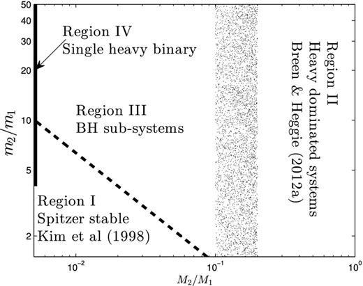
The parameter space of two-component systems divided up into different regions depending on their structure and the conditions for the onset of gravothermal oscillations. See the text and Table 8 for details.
Gravothermal oscillations in Spitzer stable systems were studied by Kim et al. (1998). They argued that because of the small values of M2/M1 (and the high values of m2/m1), the heavy component was confined to the centre of the system. They showed that the systems they studied became gravothermally unstable once a certain ratio of energy flux at rh and rc (i.e. ϵ) was reached, and that this value was the same as that for a one-component system. As the bulk of the system is in the light component, this implies that the instability results from a large isothermal region in the light component. These remarks justify the entries in row 1 of Table 8.
One situation where the concept of Spitzer stability is inappropriate is where the number of heavy particles is small (N ∼ 2). As the heavy particles tend to find their way to the core of the system and form a binary, the role of the heavy component is still significant, because this binary becomes the power source for the system lying inside the core of the light system. That is why these systems have been given their own classification, although they may be regarded as the extreme of low M2/M1 for both Spitzer stable and Spitzer unstable systems. Clearly in this case if gravothermal oscillations are found, they will result from a large isothermal region in the light component, hence the entries in the last row of Table 8.
Finally, the last division in Fig. 16 is between regions II and III. The space occupied by regions II and III consists entirely of Spitzer unstable models. The difference between these two models depends on the value of M2/M1. The case where M2 ≪ M1 includes the topic of interest in this paper (i.e. systems containing BH subsystems). Due to small M2/M1 in these systems, the light component dominates at rh and thus the rate of energy generation is regulated by the light component. In the case where M2 ≳ 0.1M1, the heavy component has a significant effect on the relaxation process within rh, particularly when M2 ∼ M1 (Breen & Heggie 2012a). The distinction between the two cases is clear when considering extreme values of M2/M1, but the exact division between the two is unclear and may have some dependence on m2/m1. This is why a shaded area separates the two regions in Fig. 16. In both cases, the onset of gravothermal instability is associated with a large isothermal region in the heavy component (see Section 5 in this paper and Breen & Heggie 2012a). Another reason for the distinction between regions II and III is the theoretical arguments given in Section 2.6: if we consider tidally limited systems, M2/M1 is expected to grow with time for region II systems and decrease with time for region III systems.
We thank S. Portegies Zwart for numerous helpful comments on a previous draft of this paper. Some of our hardware was purchased using a Small Project Grant awarded to DCH and Dr M. Ruffert (School of Mathematics) by the University of Edinburgh Development Trust, and we are most grateful for it. PGB is funded by the Science and Technology Facilities Council (STFC).
Note that there is an error in Heggie & Hut (2003, p. 225): the constant is stated incorrectly but the correct value can be obtained by evaluating the formula given on the same page.
REFERENCES
APPENDIX A: ENERGY TRANSPORT IN SYSTEMS CONTAINING A BH SUBSYSTEM
It has been a fundamental assumption in this paper that, in a system containing a BH subsystem, the majority of energy generated first flows throughout the BH subsystem and is then transferred to the rest of the system via two-body relaxation. In this section we will discuss the validity of such an assumption. We will do this by considering the energy generated by a BH binary as it hardens and is ultimately ejected from the system, as was done for the one-component case by Heggie & Hut (2003). We shall assume that the BH binary mostly generates energy by encounters with a single BH. This is a reasonable assumption as long as there are sufficient BH for the central region to be dominated by them. We can divide the life of the BH binary in the system into five energy generating phases as follows.
After the BH binary is formed, the interactions between the binary and the other BH will not be energetic enough to remove either from the subsystem. During this phase all the energy that is generated must be deposited within the BH subsystem.
After phase 1 the binary then starts giving the single BH enough energy to escape the BH subsystem. The single BH will typically receive more kinetic energy from an encounter with a BH binary than the binary itself. During this phase the BH binary remains in the BH subsystem and the increase in the kinetic energy of the centre of mass (c.m.) of the binary is deposited in the BH subsystem. Some of the energy of the single BH, however, is deposited directly into the light component though how much is discussed further below.
At some point the c.m. of the BH binary will receive enough kinetic energy that it too can escape from the BH subsystem along with the single BH. As the density is much lower outside the BH subsystem, however, the binary is unlikely to deposit much energy until it returns to the higher density region in the centre of the BH subsystem.
The single BH starts receiving enough energy to escape from the system. The BH binary still escapes from the BH subsystem but remains bound to the whole system and ultimately returns to the BH subsystem.
Finally, the BH binary escapes from the system and the binary contributes no more energy to the system.
Using the same approach as Heggie & Hut (2003, see p. 225, box 32.1), we will now consider where the energy generated by each hard binary is distributed. As stated in Section 2.5, the amount of energy generated by each hard binary is expected to be ∼10m2|ϕc| and we will assume as in Section 2.5 that ϕ2/ϕ1 ≈ 10−1. We will consider in turn heating from BH which do not escape the subsystem, from subescapers (BH which escape from the subsystem but not from the system) and finally from BH which escape the system.
Heating from BH which do not escape the subsystem is involved in phases 1 (the single BH and the binary) and 2 (the binary). The amount of energy generated during phase 1 can be estimated in the same way as was done for the one-component case by Heggie & Hut (2003). The result is that only about 3 per cent of the total energy generation per hard binary is generated during this phase. Including the direct heating by the BH binary during phase 2, the total heating from BH which do not escape the subsystem is about 5.5 per cent.
Heating from subescapers is involved in phases 2 (the single BH), 3 (the single BH and the binary) and 4 (the binary). The total amount of energy contributed by subescapers is about 49 per cent. Initially, a subescaper indirectly heats the BH subsystem, by m2ϕ2 for a single BH and by 2m2ϕ2 in the case of the binary. The number of single subescapers is expected to be approximately 4.3 and the number of encounters which cause the binary to become a subescaper is also approximately 4.3. This is because in both cases 4.3 is the typical number of encounters needed to increase the binding energy of the binary by a factor of 10. This brings the total amount of heating (including the direct heating considered previously) to the BH subsystem to 18 per cent.
What happens to a subescaper once it leaves the BH subsystem is a point of uncertainty. It will indirectly heat the light component up to some maximum radius (which depends on its kinetic energy) reached by the BH. It is possible that afterwards the subescaper remains on a nearly radial orbit and falls back into the BH subsystem, releasing most of its energy there. In the case of one-component systems, Spitzer (1987) showed that if a particle is ejected from the core, its orbit is perturbed by the other stars in the system, with the result that the particle misses the core at the next pericentre of its orbit. However, it is clear that the more massive BH will be less significantly perturbed by the light stars in the system, and may well return to the subsystem at the pericentre of its orbit. If the BH does return to the subsystem, then most of its energy will be distributed there, and the same reasoning will also apply to non-escaping BH binaries which are ejected from the core. If almost all the heating from subescapers occurs in the BH subsystem, then the total heating per binary (including the other heating considered previously) to the BH subsystem is ≈54 per cent.
Finally, it is fairly easy to estimate the amount of energy resulting from escapers, which is m2|ϕc| per single BH escaper and 2m2|ϕc| for the escape of the binary itself. The heating is indirect and heating to each component is proportional to the contribution of each component to the central potential. Per hard binary the percentage of energy generated due to escape is the same as for a one-component system, and is approximately 45 per cent: of this about 10 per cent goes into the heating of the BH subsystem (as ϕc − ϕc,1 ≃ 0.1ϕc). This type of heating is involved in phases 4 (the single BH) and 5 (the binary and single BH). Therefore, the heating to the BH subsystem per hard binary may be as much as 59 per cent. We have assumed (Sections 2.1 and 2.2) that all energy heats the BH subsystem and is then conducted to the light component. Clearly this assumption is only approximately valid if the proportion of heating to the BH subsystem (per BH binary) is ∼59 per cent.
APPENDIX B: HEATING IN OUTER LAGRANGIAN SHELLS
In this section we shall consider the heating by the BH caused by the initial mass segregation. In simulations in this paper, the BH are initially spread throughout the system with the same velocity distribution as the other stars. As the BH are much more massive than the other stars, the tendency towards equipartition of kinetic energy causes the BH to lose kinetic energy to the other stars, which in turn causes the BH to fall in the potential well of the cluster. As stated in Section 2, these systems are usually Spitzer unstable, and therefore equipartition of kinetic energy cannot be achieved: BH continuously fall in the potential well until they are concentrated in the centre of the system. The time this process takes depends on the location of the BH, as the process depends on the local relaxation time, which varies significantly throughout the cluster. For BH which start in the outer parts of the system, this process takes the longest, as the relaxation time is the longest there and they have to travel the furthest to reach the central region.
For BH whose orbits lie mostly outside the half-mass radius of the whole system, the loss of energy causes an increase in the mean kinetic energy, just as for orbits in a 1/r potential. Also, the relaxation time at the location of these BH considerably exceeds the half-mass relaxation time. Though the equipartition time-scale is smaller by a factor of m1/m2, there is some radius outside the half-mass radius at which the equipartition time-scale is comparable with the time of core collapse which, for parameters of our typical models, can be taken to be roughly 0.3trh. Throughout core collapse, therefore, we can expect the outermost Lagrangian radii of the BH component to exhibit a steady rise in velocity dispersion, while in intermediate Lagrangian shells the velocity dispersion first increases and then decreases. In the innermost Lagrangian shells, the velocity dispersion may be expected to decrease throughout the time to the first core collapse.
This behaviour is illustrated in Fig. B1 with an N-body run. This run uses m2/m1 = 5, which is smaller than what would be expected for a BH subsystem; however, the small value of m2/m1 allows for a large value of N2 (in this case N2 = 1000), which more clearly illustrates the behaviour. As can be seen in Fig. B1 (bottom), the squared three-dimensional velocity dispersion (|$v_2^2$|) initially decreases for the Lagrangian radii within ∼rh and initially increases for the larger Lagrangian radii. The heating in the outer Lagrangian radii ends roughly when the radii enter rh (see Fig. B1, top), after which they show a decrease in v2 up until t ≈ 2500, when there is an increase in v2 which is associated with core collapse. By the time that core collapse has completed (at t ≃ 3250), most of the BH (80 per cent) have been segregated to within ≈0.2rh. At this time, the outermost Lagrangian radius (90 per cent of M2) has the highest value of v2 (Fig. B1, bottom), though part of the increase may be attributable to BH ejection. The outermost BH still undergo mass segregation. Indeed, as can be seen in Fig. B1 (top), the outermost Lagrangian radius continuously contracts even after core collapse occurs.
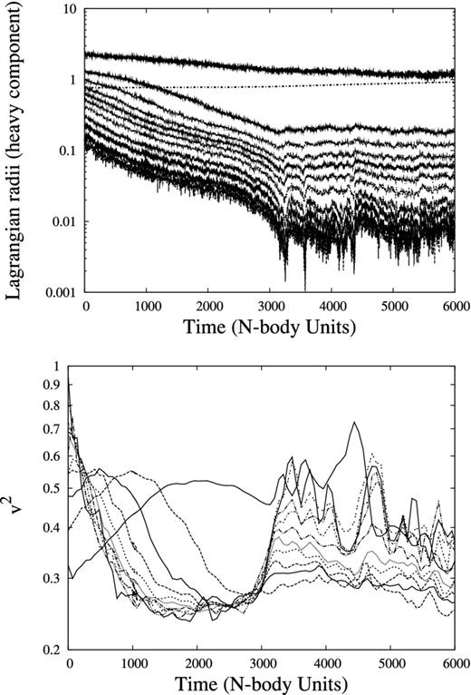
Evolution of the heavy component in a two-component N-body run with initial values N = 128k, m2/m1 = 5 and M2/M1 ≈ 0.038. The corresponding mass fractions are 1, 2, 5, 10, 20, 30, 40, 50, 62.5, 75 and 90 per cent of M2. Bottom: mean-square velocity dispersion inside the Lagrangian shell. The 90 per cent shell becomes the hottest shell at t ≃ 1450 and remains hotter than the next inner shell until well after tcc. Top: plot of the radii of the Lagrangian shells in the heavy component. The dotted line is rh, the half-mass radius of the whole system.
The behaviour discussed in this section is not limited to systems containing a BH subsystem; in fact any system with a mass spectrum should also exhibit similar behaviour. The important point is that continued mass segregation serves to heat the low-mass component, and this kind of heating may lower the required rate of energy generation from the core, as energy is directly injected into the region near rh. This effect has not been taken into account in the theory in Section 2, but as the values of N2 are so small in Section 2, it is unlikely that this effect is significant.
