


Abstract
This is the third paper of a series reporting the results from the popstar evolutionary synthesis models. The main goal of this work is to present and discuss the synthetic photometric properties of single stellar populations resulting from our popstar code. Colours in the Johnson and Sloan Digital Sky Survey (SDSS) systems, Hα and Hβ luminosities and equivalent widths, and ionizing region size, have been computed for a wide range of metallicity (Z = 0.0001–0.05) and age (0.1 Myr to 20 Gyr). We calculate the evolution of the cluster and the region geometry in a consistent manner. We demonstrate the importance of the contribution of emission lines to broader band photometry when characterizing stellar populations, through the presentation of both contaminated and non-contaminated colours (in both the Johnson and SDSS systems). The tabulated colours include stellar and nebular components, in addition to line emission. The main application of these models is the determination of physical properties of a given young ionizing cluster, when only photometric observations are available; for an isolated star-forming region, the young star cluster models can be used, free from the contamination of any underlying background stellar population. In most cases, however, the ionizing population is usually embedded in a large and complex system, and the observed photometric properties result from the combination of a young star-forming burst and the underlying older population of the host. Therefore, the second objective of this paper is to provide a grid of models useful in the interpretation of mixed regions where the separation of young and old populations is not sufficiently reliable. We describe the set of popstar spectral energy distributions (SEDs), and the derived colours for mixed populations where an underlying host population is combined in different mass-ratios with a recent ionizing burst. These colours, together with other common photometric parameters, such as the Hα radius of the ionized region, and Balmer line equivalent widths and luminosities, allow one to infer the physical properties of star-forming regions even in the absence of spectroscopic information.
INTRODUCTION
For many years, broad-band photometry was used as the primary tool in deriving ages for both single bursts and mixed stellar populations. Broadly speaking, blue colours were taken to be indicative of young populations, while red colours were associated with older populations. Only dust was thought to complicate this picture, through the general reddening of the population. From an observational perspective, a few works have considered the potential contaminating impact of gas emission upon broad-band colours. For example, López-Sánchez & Esteban (2008) analysed carefully colour–colour diagrams, taking into account this correction, and thereby proposing a mechanism for separating the contribution from the underlying stellar population, starburst population, and line emission, for better quantitative comparison with evolutionary models of stellar populations. From a theoretical perspective, colours were calculated typically for the stellar component only or, in a few cases, by taking into account the nebular continuum. Only recently, several works (Martín-Manjón et al. 2008; Reines et al. 2010, and references therein) have started to quantify the role of line emission from ionized gas surrounding young star clusters in the contamination of broad-band colours. These latter authors examined two young massive clusters in NGC 4449, demonstrating that the contribution of both nebular continuum and line emission is essential to reproduce the observed broad-band fluxes. The comparison of model spectral energy distributions (SEDs) with and without nebular continuum and/or emission lines shows that the inferred stellar mass can change by up to a factor of ∼2.5, depending upon the filter in question. Atek et al. (2011) also find that nebular lines can contaminate the total broad-band flux by ∼0.3 mag (median, but up to ∼1 mag, in certain cases). This effect is important since low-redshift galaxies with active star formation may mimic the colour-selection criteria used in some high-redshift dropout surveys. This potential impact on the mass and age of galaxies is also important for cosmological studies which use these values as clues to disentangle the temporal history of galaxy assembly. Despite this importance, to our knowledge there is no available systematic grid of models which includes the effect of emission lines on broad-band colours spanning a wide range in age and metallicity [but see Adamo et al. (2010), who compute some colours for the Hubble Space Telescope by including the emission lines for Z = 0.0004 SEDs from starburst99 to explain the red excess observed in SBS 0335–052E super star clusters]. Our work has been designed to fill this gap.
Over the past two decades, a wealth of powerful ground-based facilities, particularly in the visible, has driven the use of spectroscopic techniques to infer the underlying physical properties of ionizing star clusters. High signal-to-noise spectra were required, in order to derive the nebular electron density and electron temperature, and from these gas parameters, the abundance. In the absence of a consistent grid of models against which to compare, photometric information has not been used as the main tool for deriving star-forming properties. In terms of observations, there were a few consistent samples of H ii regions (or small- to medium-size star-forming objects) that would allow us to test models and from which we could extract statistical conclusions. Moreover, these existing observational samples were usually biased towards bright and low-to-intermediate-metallicity regions. This subject has been exhaustively discussed by Martín-Manjón et al. (2010, hereafter Paper II), in which we presented the emission-line spectra for our models as a function of the physical properties of the ionizing clusters and compared the resulting diagnostic diagrams with a complete spectroscopic sample of H ii regions for which abundances were derived consistently using an appropriate empirical calibration.
The recent generation of deep surveys, taken with mid-to-large aperture telescopes, have now released complete photometric catalogues of star-forming regions and galaxies at different redshifts. This has motivated us to deliver a set of models which can aid in the derivation of the physical properties of stellar populations, without the necessity of spectroscopic data. With this in mind, we have computed the colours and other common photometric parameters, such as Hα radius, Hα and Hβ equivalent widths and Hα and Hβ luminosities. We are convinced that these models will be a powerful tool in the interpretation of star-forming region photometric data, providing the means to infer their mass, age and metallicity when embedded within more complex and evolved systems.
We have computed colours previously with the popstar SEDs in both Johnson and Sloan Digital Sky Survey (SDSS) systems (Mollá, García-Vargas & Bressan 2009, hereafter Paper I). We present now the colour evolution of star-forming regions formed by a single stellar population (SSP), including the contribution of the strongest emission lines from the ionized nebula, which can be used to derive the physical properties of the ionizing clusters. These SSP models can be used directly to compare with specific, usually small and detailed, photometric samples, where colours have been corrected for the contamination from an underlying population. However, this is not the general case, since the subtraction of the underlying population delivers results that are not always reliable; furthermore, this approach is not the most commonly used one when a large amount of data, like the output of extremely large surveys, are analysed. Such surveys are used to obtain statistical conclusions about the star-forming regions, and therefore the use of appropriate theoretical models is essential. For this reason, in addition to the SSP models, we have also computed a complete set of photometric properties for mixed populations, to simulate local star-forming regions embedded in more complex star systems. These models are particularly useful when the subtraction of an underlying population is not sufficiently reliable.
This paper describes the photometrical model and demonstrates how photometry can be an alternative and powerful tool in the delivery of inferred ages and metallicities for star-forming regions, as well as how it can give an estimation of the mass-ratio of the star-forming region to that of the underlying population. The models presented here are applicable to nearby/local star-forming regions only, since the contribution of the emission lines varies with redshift. It is obvious that the most important emission lines contaminate different filters, with different transmittance, as a function of redshift. We outline the importance of an extension of this work to higher redshift, to study the impact of emission lines on broad-band photometry of samples at different redshift. Dust re-emission and near-IR photometry will be also included to extend the use of the models to large samples covering a wide range of redshifts.
Section 2 summarizes the main properties of the grid of evolutionary synthesis models used to compute the magnitudes of pure SSPs, the method to calculate the emission-line intensities of the photoionized nebula and, consequently, the associated contaminated colours. Section 3 presents and analyses the results of our models for young ionizing SSPs. These models can be used for deriving the physical properties of the ionizing populations in regions whose observed colours have been previously de-contaminated from the underlying populations. Section 4 describes the set of models for mixed populations, applicable to characterizing star-forming regions where these bursts are placed on an underlying population and where we cannot separate both components observationally. Finally, Section 5 summarizes our results.
SSP COLOUR CALCULATIONS
popstar model summary
A detailed description of popstar can be found in Paper I. popstar provides a set of evolutionary synthesis models for SSPs, covering a wide range in age and metallicity. The basic grid is composed of SSPs for six different initial mass functions (IMFs). For this work, we have used only a Salpeter IMF (Salpeter 1955) with lower and upper mass limits of 0.15 and 100 M⊙, respectively. We have not included binaries nor mass segregation.
The isochrones employed are updated versions of those from Bressan, Granato & Silva (1998) for six metallicities: Z = 0.0001, 0.0004, 0.004, 0.008, 0.02 and 0.05. The use of very low metallicity models (Z = 0.0001) was not included in comparable work prior to that of popstar. The age ranges from log τ = 5.00 to 10.30 with a variable time resolution reaching Δ(log τ) = 0.01 in the youngest populations. Again, details of the isochrones are described in Paper I.
Stellar atmosphere models are taken from Lejeune, Cuisinier & Buser (1997), due to its expansive coverage in effective temperature, gravity and metallicities for stars with Teff ≤25000 K. For O, B and WR stars, the non-local thermodynamic equilibrium (NLTE) blanketed models of Smith, Norris & Crowther (2002b), for metallicities Z =0.001, 0.004, 0.008, 0.02 and 0.04, are used. There are 110 models for O-B stars, calculated by Pauldrach, Hoffmann & Lennon (2001), with 25 000 < Teff ≤ 51 500 K and 2.95 ≤ log g ≤ 4.00, and 120 models for WR stars (60 WN and 60 WC), from Hillier & Miller (1998), with 30 000 ≤ T* ≤ 120 000 K and 1.3 ≤ R* ≤ 20.3 R⊙ for WN, and with 40 000 ≤ T* ≤ 140 000 K and 0.8 ≤ R* ≤ 9.3 R⊙ for WC. T* and R* are the temperature and the radius at a Roseland optical depth of 10. The assignment of the appropriate WR model is consistently made by using the relationships between opacity, mass-loss and velocity wind, as described in Paper I. For post-asymptotic giant branch and planetary nebulae with Teff between 50 000 and 220 000 K, the NLTE models from Rauch (2003) are taken. For higher temperatures, popstar uses black-bodies. The use of these latter models modifies the resulting intermediate-age SEDs.
For each cluster, the total mechanical energy from stellar winds and supernova (SN) has been calculated. We have used this mechanical energy to calculate the H ii region's inner radius (see Section 2.2). We have also computed the nebular continuum emission from hydrogen and helium (He and He+) free–free, free–bound and two-photon continuum emission.
The SEDs (stellar+nebular) corresponding to the six metallicities and ages up to 20 Myr have been introduced to the photoionization code cloudy (Ferland et al. 1998) to obtain the emission-line spectra (see Paper II for details). We take seven possible cluster masses: 1.2 × 10⁴, 2.0 × 10⁴, 4.0 × 10⁴, 6.0 × 10⁴, 1.0 × 10⁵, 1.5 × 10⁵ and 2.0 × 10⁵ M⊙ selected to cover the Hα luminosity range observed for medium-to-large H ii regions. The gas surrounding the cluster is assumed to have the same chemical composition as the stars of the cluster. For each metallicity, the element abundances heavier than helium have been scaled by a constant factor, with respect to the hydrogen content, according to the solar abundances from Grevesse & Sauval (1998) and depleted when necessary (see table 2 from Paper II). The models assume a bubble geometry, with an ionized bounded nebula whose size is given by the cluster evolution. Therefore, the internal radius of the shell is the distance at which the ionized gas is deposited in that nebula by the cluster's mechanical energy. Be aware that the observed radius of an H ii region is not necessarily the inner radius of the ionized region (see Section 2.2). The effect of dust here has not been included.
The hydrogen density has been considered constant throughout the nebula and equal to the electron density for complete ionization. We have generated models assuming two different values of electron density, nH: 10 and 100 cm−3, in order to quantify the impact of density on the emitted spectrum. A density of 10 cm−3 is more appropriate for small–medium isolated H ii regions while 100 cm−3 is more appropriate for H ii galaxies, large circumnuclear H ii regions, often found around the nuclei of starbursts, or AGN. Although the constant density hypothesis is not realistic when detailed nebular studies are done, it can be considered representative when the integrated spectrum of the nebula is analysed. Results from the photoionization models and their application to spectroscopic observations of H ii regions are widely discussed in Paper II.
The number of ionizing photons, Q(H), and the Hα and Hβ luminosities have been calculated in Paper I. The equivalent width of Hα and Hβ are here calculated from the single population plus the nebular continuum (in the case of SSPs) or from the sum of all stellar populations plus nebular continuum, in the case of mixed populations (Section 4). From the computed SEDs, we previously calculated their corresponding total (stellar + nebular) uncontaminated colours in Paper I; now, using the cloudy output, we compute the colours including the contamination from emission lines, as described in Section 2.3.
Basic properties of H ii regions: sizes and luminosities
Throughout this work, we assume a scenario in which sufficient gas exists to be ionized (i.e. matter-bounded models have not been considered) and in which the birth of a star cluster, which we consider to be placed in the centre of a spherical region, is produced. In fact, we will not be able to detect the region in the visible until the neutral gas has started to ionize, allowing detection of the emission lines (in particular the Balmer lines). For that, we need to have not only ionizing photons but also certain nebula conditions, including a given gas density and an optical depth for the emitting region. These conditions occur around 0.5–1.0 Myr after cluster formation. As cluster evolves, the mechanical energy of the massive stars winds begins to sweep the gas away, compressing it and producing a shell. The wind-driven shell begins then to evolve with an initial phase of free expansion, followed by an adiabatic expansion phase, and then the swept-up material collapses to a thin, cold shell as a result of radiative cooling (e.g. Gibson 1994; Tenorio-Tagle et al. 1999).
Computed radii for the modelled stellar clusters of Z = 0.008 at selected ages for ne = 10 cm−3. Complete table for ne = 10 and 100 cm−3 and all ages and metallicities can be found online.
| Z | log τ | Mcl | Rin | ΔR | Rout |
|---|---|---|---|---|---|
| (yr) | (104 M⊙) | (pc) | (pc) | (pc) | |
| ne = 10 cm−3 | |||||
| 0.008 | 6.30 | 1.2 | 45.440 | 1.72e+01 | 62.649 |
| 0.008 | 6.30 | 2.0 | 50.320 | 2.34e+01 | 73.717 |
| 0.008 | 6.30 | 4.0 | 57.810 | 3.55e+01 | 93.261 |
| 0.008 | 6.30 | 6.0 | 62.690 | 4.53e+01 | 108.005 |
| 0.008 | 6.30 | 10.0 | 69.440 | 6.16e+01 | 131.017 |
| 0.008 | 6.30 | 15.0 | 75.300 | 7.85e+01 | 153.832 |
| 0.008 | 6.30 | 20.0 | 79.760 | 9.33e+01 | 173.100 |
| 0.008 | 6.40 | 1.2 | 51.980 | 1.10e+01 | 62.994 |
| 0.008 | 6.40 | 2.0 | 57.570 | 1.50e+01 | 72.541 |
| 0.008 | 6.40 | 4.0 | 66.130 | 2.27e+01 | 88.873 |
| 0.008 | 6.40 | 6.0 | 71.720 | 2.90e+01 | 100.717 |
| 0.008 | 6.40 | 10.0 | 79.440 | 3.94e+01 | 118.846 |
| 0.008 | 6.40 | 15.0 | 86.150 | 5.02e+01 | 136.399 |
| 0.008 | 6.40 | 20.0 | 91.250 | 5.99e+01 | 151.115 |
We have therefore calculated the shell thickness, ΔR, and the outer radius, Rout (the sum of the inner radius plus the shell thickness). Table 1 partially shown here summarizes the results for the modelled stellar clusters of Z = 0.008 at selected ages and ne = 10 cm−3. The complete Table 1, available in electronic format, for all ages and metallicities, is computed for two values of the ionizing gas electron density, since this parameter influences both the inner radius and the shell thickness: ne = 10 and 100 cm−3. In each one, columns list the metallicity Z, the logarithm of the age log τ (in yr), the cluster mass Mcl (in units of 104 M⊙), the H ii region inner radius Rin (in pc), the shell thickness ΔR (in pc) and the total radius of the region Rout (in pc), this latter radius being the most appropriate when comparing with real photometric radii observed in most H ii regions (usually measured from Hα images).
The evolution of Rin is plotted in Fig. 1. At the beginning of the cluster's evolution, the inner radius is small and the shell thickness is very large, as shown in Fig. 2, so that photons cannot escape. At a certain age (around 0.5 Myr), we start to detect the region by the emission-line luminosity classifying it like a classical H ii region. As the cluster evolves and its mechanical energy increases, the inner radius becomes larger while the shell becomes thinner. We will still see the region with a different emission-line spectrum resulting from the cluster evolution (that changes both the ionizing spectrum and the region geometry). We identify the observed object as an H ii region (by definition) if we can detect hydrogen in emission, and this happens even after the emission line spectrum of forbidden lines is over and up to 20 Myr (in average because there is a metallicity dependence).

Region inner radius evolution: Rin (pc) versus cluster age (in Myr) for six different metallicities as labelled and different cluster mass, plotted in different colours. Cluster masses of 0.12, 0.20, 0.40, 0.60, 1.00, 1.50 and 2.00 × 10⁵ M⊙ have been plotted in yellow, orange, red, green, cyan, blue and purple, respectively. The IMF is that of Salpeter with mlow = 0.15 M⊙ and mup = 100 M⊙. Panel (a) shows models using a value of the gas electron density of ne = 10 cm−3, while in panel (b) they are computed with ne = 100 cm−3.
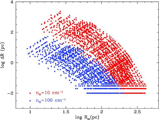
Shell thickness versus inner radius Rin (pc) for all metallicities, cluster masses and ages up to 20 Myr. Models with ne = 10 cm−3 are plotted in red while models with ne = 100 cm−3 are plotted in blue.
The external radius of the region, which we would identify as the observed one in most photometric observations, is plotted against age in Fig. 3. In this figure, we can see the differences compared to Fig. 1. This radius starts with a value of around hundreds of pc, smaller for ne = 100 cm−3, and then decreases until SNe explosions begin to appear, which increase again the size of the region. Once the SNe explosions start to appear in the region, they can change the appearance and/or the geometry; however, we then should be more cautious when interpreting the observations based on our models, since the emission line spectrum will be the result of the shock and the photoionization mechanisms. Our models do not include a shock contribution that can affect some emission lines, including [O i] 6300 Å.
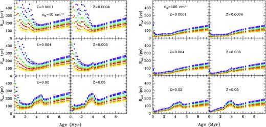
Region external radius evolution: Rout (pc) versus cluster age (Myr) for six different metallicities, all ages up to 20 Myr and different cluster's mass, using the same colour coding that in Fig. 1.
Besides the evolution of the radius of the region measured on the Hα images, we show in Figs 4 and 5 the evolution of the intensity and equivalent width of Hα. In Fig. 4, we see that Hα luminosity maintains a high level for ages longer than 5 Myr and it maintains a detectable intensity until 20 Myr for the lowest abundances. This fact will have an impact on the colours, as we will see in the next section. The equivalent width shows a similar decreasing dependence with age, but also shows high values after the first 5.5 Myr for Z = 0.0001 and Z = 0.0004, while it falls to zero for the other abundances.
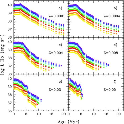
Hα evolution: log L Hα (erg s−1) versus cluster age (Myr) for six different metallicities and different cluster masses, plotted using the same colour coding that in Fig. 1.
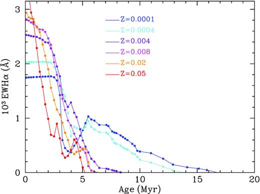
EW Hα evolution: EW Hα (Å) versus cluster age (Myr) for six different metallicities as labelled.
Fig. 6 shows the outer radius of the region as a function of the logarithm of Hα luminosity. Models for different cluster masses are represented with different colours, as before. We see that H ii regions may be quite large in size and luminosities for the lowest abundances compared with the metal-rich regions. Therefore, if these regions are not observed, we need to consider potential observational selection effects. On the contrary, the metal-rich H ii regions are much smaller, implying difficulty in observing these regions.
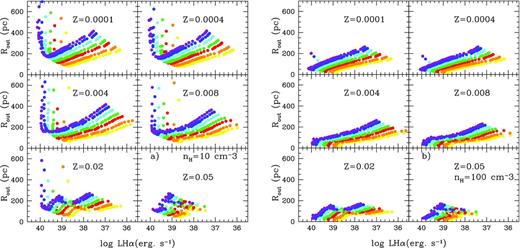
Hα evolution: R (pc) versus log (L Hα) (erg s−1) for six different metallicities and different cluster masses. Cluster masses have been plotted using the same colour coding as that in Fig. 1. Panel (a) on the right shows models computed for a gas electron density of ne = 10 cm−3, while panel (b) on the left uses a value of ne = 100 cm−3.
It seems that an inverse correlation between size and luminosity arises from these plots for luminosities lower than 1040 erg s−1 if the evolution of one cluster mass is followed, with larger radii for longer evolutionary times, when the Hα luminosity decreases. Observations instead show a positive correlation between size and luminosity. In fact, our results are restricted due to the cluster masses selected in our computations. In Fig. 7(a), we show as coloured points our results (with the same code than in Fig. 6) only for models with ΔR > 0.5 pc. This selection of models constrains the resulting luminosities to the range 1038–1040 erg s−1. We compare these models with data from Mayya (1994), Ferreiro & Pastoriza (2004), Hakobyan et al. (2007) and Martínez-Delgado (2009), shown as grey symbols. We see that some data fall out of the region defined by our models. In fact, observational points (which proceed from H ii regions of different galaxies) show an abrupt decrease at a given luminosity, followed by a smooth increase that indicates the transition time in which massive star winds disappear and SNe start to increase the size of the bubble. However, some observational points seem to affect this change at an Hα luminosity higher than our models have. Thus, most observations from Ferreiro & Pastoriza (2004) show a behaviour that would be reproduced by models with a cluster mass larger than 2 × 10⁵ M⊙, our maximum cluster mass, or with a different IMF. Differences in the mass limits or slope of the IMF will change the mass distribution in the cluster generation, with direct consequences on the number of ionizing photons and LHα. This effect was discussed in Paper I (Mollá et al. 2009). On the other end, many data from Mayya (1994) need a cluster mass smaller than 1.2 × 10⁴ M⊙, the lowest limit of the models computed here. These latter observations show a similarly strong increase around LHα ∼ 1038 erg s−1, slightly smaller than that shown by the lowest cluster mass model. Therefore, in panel (b), we compare our models only with the other two sets of data from Hakobyan et al. (2007) and Martínez-Delgado (2009) fitted by ionized clusters whose masses are within our model range. Doing so, we see that the observed correlation between size and luminosity is reproduced with our models, the dispersion for which is driven by the range in cluster masses. In that panel, the red line represents the least-squares straight fit to the data while the black line represents the corresponding one for models. However, we warn that this correlation is not totally due to an evolutionary effect – as it has been argued in previous works – but a combination of the evolutionary state (age) and the mass of the cluster. A model with a given cluster mass shows a decrease in the size, while decreasing the Hα luminosity, before the SNe explosion time. Then, a new increase in the size of the region is seen (see Fig. 6), while the Hα luminosity continues to decrease. Only when all cluster masses are included in the same plot (Fig. 7b) does the correlation between radius and luminosity arise clearly (e.g. Fig. 7b), showing, in the plane log Rout-log LHα, a slope similar to the observed one.
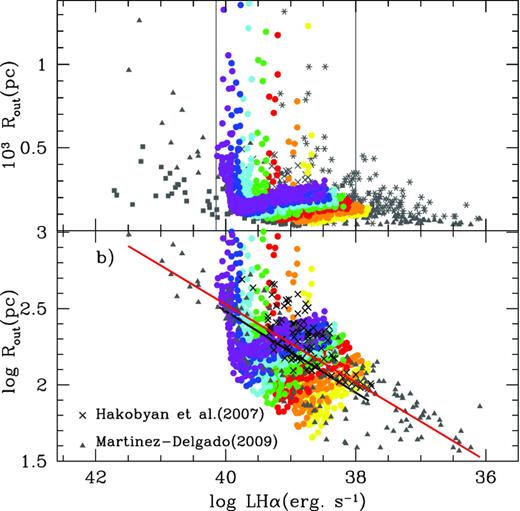
Relation of the outer radius Rout versus the Hα luminosity compared with observations. The coloured full dots are our models for nH = 10 cm−1, selecting those with ΔR ≥ 0.5 pc. In panel (a), grey symbols represent the observational data from Mayya (1994), Ferreiro & Pastoriza (2004), Hakobyan et al. (2007) and Martínez-Delgado (2009) as asterisks, filled squares, crosses and filled triangles, respectively. In panel (b), with both axis in logarithmic scale, the (grey) triangles represent data from Martínez-Delgado (2009) and the (black) crosses represent data from Hakobyan et al. (2007). The red and black lines indicate the corresponding least-squares fit to the data set and models, respectively.
Colour calculation
The filters included in this work are the optical broad-band associated with Johnson's system (UBVRI) and the SDSS (ugriz) system. The transmission curves for both are shown in Fig. 8. Table 2, for which we show an example, and given in electronic format only, contains the transmission values as a function of wavelength for Johnson and SDSS filters.
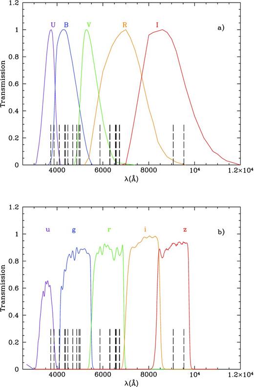
Transmission curves of (a) U, B, V, R and I broad-band Johnson filters and (b) u, g, r, i and z SDSS system filters. The figure also shows the location of the emission lines contributing to these filters.
Transmission value T of Johnson and SDSS filters. The complete table can be found in the online version.
| λ | T |
|---|---|
| (Å) | |
| 3050.0 | 0.000 |
| 3100.0 | 0.020 |
| 3150.0 | 0.077 |
| 3200.0 | 0.135 |
| 3250.0 | 0.204 |
| 3300.0 | 0.282 |
| 3350.0 | 0.385 |
| 3400.0 | 0.493 |
| λ | T |
|---|---|
| (Å) | |
| 3050.0 | 0.000 |
| 3100.0 | 0.020 |
| 3150.0 | 0.077 |
| 3200.0 | 0.135 |
| 3250.0 | 0.204 |
| 3300.0 | 0.282 |
| 3350.0 | 0.385 |
| 3400.0 | 0.493 |
The emission lines considered in this work are 3727 [O ii], 3869 [Ne iii], 4101 Hδ, 4340 Hγ, 4363 [O iii], 4471 He i, 4686 He ii, 4861 Hβ, 4959 [O iii], 5007 [O iii], 5871 He i, 6300 [O i], 6312 [S iii], 6548 [N ii], 6563 Hα, 6584 [N ii], 6716 [S ii], 6731 [S ii], 9069 [S iii] and 9532 [S iii]. The transmission of the selected broad-band filters at these wavelengths is given in Table 3. Fig. 8 shows the filter transmission curves. Panel (a) shows the UBVRI Johnson filters while panel (b) shows the ugriz SDSS filters. We have marked in both panels the position of the 20 selected emission lines at z = 0. We remind the reader that the use of these models is only valid for local, low-redshift systems. For more distant objects, the shift of the lines has to be taken into account since the transmission of the filter at the wavelength of a given emission line (and therefore the contribution to the integrated colour) will also vary with redshift. We will discuss these effects in a future work.
Transmission of the broad-band filters at the rest wavelength of the selected emission lines.
| Emission line | T at U | T at B | T at B | T at V | T at R | T at I | T at u | T at g | T at r | T at i | T at z |
|---|---|---|---|---|---|---|---|---|---|---|---|
| (Å) | for U − B | for B − V | |||||||||
| 3727 [O ii] | 0.9966 | 0.0329 | 0.0438 | 0.0000 | 0.0000 | 0.0000 | 0.5781 | 0.0000 | 0.0000 | 0.0000 | 0.0000 |
| 3869 [Ne iii] | 0.7837 | 0.3321 | 0.3911 | 0.0000 | 0.0000 | 0.0000 | 0.2263 | 0.0000 | 0.0000 | 0.0000 | 0.0000 |
| 4101 Hδ | 0.0557 | 0.9556 | 0.9962 | 0.0000 | 0.0000 | 0.0000 | 0.0009 | 0.0493 | 0.0000 | 0.0000 | 0.0000 |
| 4340 Hγ | 0.0000 | 0.9983 | 0.9612 | 0.0000 | 0.0000 | 0.0000 | 0.0005 | 0.7353 | 0.0000 | 0.0000 | 0.0000 |
| 4363 [O iii] | 0.0000 | 0.9947 | 0.9507 | 0.0000 | 0.0000 | 0.0000 | 0.0000 | 0.7253 | 0.0000 | 0.0000 | 0.0000 |
| 4471 He i | 0.0000 | 0.9405 | 0.8768 | 0.0000 | 0.0000 | 0.0000 | 0.0000 | 0.8237 | 0.0000 | 0.0000 | 0.0000 |
| 4686 He ii | 0.0000 | 0.7372 | 0.6621 | 0.0000 | 0.0000 | 0.0000 | 0.0000 | 0.8748 | 0.0000 | 0.0000 | 0.0000 |
| 4861 Hβ | 0.0000 | 0.5556 | 0.4859 | 0.0943 | 0.0000 | 0.0000 | 0.0000 | 0.9004 | 0.0000 | 0.0000 | 0.0000 |
| 4959 [O iii] | 0.0000 | 0.4474 | 0.3873 | 0.3265 | 0.0000 | 0.0000 | 0.0000 | 0.8577 | 0.0000 | 0.0000 | 0.0000 |
| 5007 [O iii] | 0.0000 | 0.3934 | 0.3380 | 0.4829 | 0.0000 | 0.0000 | 0.0000 | 0.8820 | 0.0000 | 0.0000 | 0.0000 |
| 5871 He i | 0.0000 | 0.0000 | 0.0000 | 0.4638 | 0.5828 | 0.0000 | 0.0000 | 0.0000 | 0.9063 | 0.0000 | 0.0000 |
| 6300 [O i] | 0.0000 | 0.0000 | 0.0000 | 0.1200 | 0.8394 | 0.0000 | 0.0000 | 0.0000 | 0.8861 | 0.0000 | 0.0000 |
| 6312 [S iii] | 0.0000 | 0.0000 | 0.0000 | 0.1134 | 0.8447 | 0.0000 | 0.0000 | 0.0000 | 0.8855 | 0.0000 | 0.0000 |
| 6548 [N ii] | 0.0000 | 0.0000 | 0.0000 | 0.0273 | 0.9263 | 0.0000 | 0.0000 | 0.0000 | 0.8456 | 0.0000 | 0.0000 |
| 6563 Hα | 0.0000 | 0.0000 | 0.0000 | 0.0250 | 0.9304 | 0.0000 | 0.0000 | 0.0000 | 0.8625 | 0.0000 | 0.0000 |
| 6584 [N ii] | 0.0000 | 0.0000 | 0.0000 | 0.0225 | 0.9359 | 0.0000 | 0.0000 | 0.0000 | 0.8842 | 0.0000 | 0.0000 |
| 6716 [S ii] | 0.0000 | 0.0000 | 0.0000 | 0.0154 | 0.9622 | 0.0000 | 0.0000 | 0.0000 | 0.8417 | 0.0001 | 0.0000 |
| 6731 [S ii] | 0.0000 | 0.0000 | 0.0000 | 0.0148 | 0.9654 | 0.0000 | 0.0000 | 0.0000 | 0.8404 | 0.0002 | 0.0000 |
| 9069 [S iii] | 0.0000 | 0.0000 | 0.0000 | 0.0000 | 0.0314 | 0.9060 | 0.0000 | 0.0000 | 0.0000 | 0.0003 | 0.9326 |
| 9532 [S iii] | 0.0000 | 0.0000 | 0.0000 | 0.0000 | 0.0000 | 0.6210 | 0.0000 | 0.0000 | 0.0000 | 0.0003 | 0.9381 |
MODEL RESULTS FOR SSPs
Results
We have computed the colours from the pure continuum SSP SEDs (stellar+nebular), and the colours contaminated by the emission lines as described in Section 2.3. Model results for Z = 0.008 and some ages as an example are summarized in Tables 4 and 5, for Johnson and SDSS colours, respectively. The complete tables are computed for two values of the ionizing gas electron density, ne, since this parameter leads to important differences in the emission line spectrum. This is well known and widely discussed in Paper II. Tables 4 and 5 are computed for ne = 10 and 100 cm−3, respectively. These tables provide the computed colours (in Johnson and SDSS systems, respectively) together with other cluster parameters that can be obtained from photometrical observations. Table 4 columns list the metallicity Z, the logarithm of the age τ (in yr), the cluster mass Mcl (in M⊙), the logarithm of the Hβ and Hα luminosities, L Hβ and L Hα (both in erg s− 1), the absolute magnitude V and colours (U − B)c, (B − V)c, (V − R)c and (R − I)c contaminated with the emission lines, the uncontaminated absolute magnitude V, and colours U − B, B − V, V − R and R − I (which obviously do not change with the mass of the stellar cluster). Table 5 columns list the metallicity Z, the logarithm of the age τ (in yr), the cluster mass Mcl (in M⊙), the equivalent widths of Hβ and Hα, EW(Hβ) and EW(Hα) in Å, the absolute magnitude g and colours (u − g)c, (g − r)c, (r − i)c and (i − z)c contaminated with the emission lines, the uncontaminated absolute magnitude g and colours u − g, g − r, r − i and i − z. The whole table with results for all ages and metallicities will be given in electronic format.
Johnson colours evolution results for the modelled stellar clusters of Z = 0.008 at some selected ages for ne = 10 cm−3. Complete table for all ages and metallicities and for ne = 10 and 100 cm−3 can be found in the online version.
| Z | logτ | Mcl | LHβ | LHα | Vc | (U − B)c | (B − V)c | (V − R)c | (R − I)c | V | U − B | B − V | V − R | R − I |
|---|---|---|---|---|---|---|---|---|---|---|---|---|---|---|
| (yr) | (M⊙) | (erg s−1) | (erg s−1) | |||||||||||
| ne = 10 cm−3 | ||||||||||||||
| 0.008 | 6.30 | 1.2 × 10⁴ | 38.23 | 38.70 | −10.407 | −1.123 | 0.130 | 0.431 | −0.437 | −9.648 | −1.356 | −0.015 | 0.159 | 0.019 |
| 0.008 | 6.30 | 2 × 10⁴ | 38.45 | 38.92 | −10.998 | −1.060 | 0.151 | 0.365 | −0.413 | −10.203 | −1.356 | −0.015 | 0.159 | 0.019 |
| 0.008 | 6.30 | 4 × 10⁴ | 38.75 | 39.22 | −11.793 | −0.984 | 0.174 | 0.290 | −0.391 | −10.955 | −1.356 | −0.015 | 0.159 | 0.019 |
| 0.008 | 6.30 | 6 × 10⁴ | 38.93 | 39.40 | −12.256 | −0.944 | 0.186 | 0.253 | −0.384 | −11.395 | −1.356 | −0.015 | 0.159 | 0.019 |
| 0.008 | 6.30 | 1 × 10⁵ | 39.15 | 39.62 | −12.835 | −0.899 | 0.199 | 0.212 | −0.378 | −11.950 | −1.356 | −0.015 | 0.159 | 0.019 |
| 0.008 | 6.30 | 1.5 × 10⁵ | 39.33 | 39.80 | −13.293 | −0.869 | 0.208 | 0.183 | −0.377 | −12.390 | −1.356 | −0.015 | 0.159 | 0.019 |
| 0.008 | 6.30 | 2 × 10⁵ | 39.45 | 39.92 | −13.618 | −0.848 | 0.215 | 0.163 | −0.378 | −12.703 | −1.356 | −0.015 | 0.159 | 0.019 |
| 0.008 | 6.40 | 1.2 × 10⁴ | 38.15 | 38.62 | −10.166 | −1.243 | −0.028 | 0.608 | −0.493 | −9.715 | −1.288 | −0.075 | 0.104 | −0.012 |
| 0.008 | 6.40 | 2 × 10⁴ | 38.37 | 38.84 | −10.753 | −1.191 | −0.009 | 0.540 | −0.459 | −10.270 | −1.288 | −0.075 | 0.104 | −0.012 |
| 0.008 | 6.40 | 4 × 10⁴ | 38.67 | 39.15 | −11.545 | −1.124 | 0.015 | 0.462 | −0.427 | −11.022 | −1.288 | −0.075 | 0.104 | −0.012 |
| 0.008 | 6.40 | 6 × 10⁴ | 38.85 | 39.32 | −12.005 | −1.088 | 0.028 | 0.423 | −0.413 | −11.462 | −1.288 | −0.075 | 0.104 | −0.012 |
| 0.008 | 6.40 | 1 × 10⁵ | 39.07 | 39.55 | −12.582 | −1.047 | 0.041 | 0.381 | −0.400 | −12.017 | −1.288 | −0.075 | 0.104 | −0.012 |
| 0.008 | 6.40 | 1.5 × 10⁵ | 39.25 | 39.72 | −13.038 | −1.018 | 0.051 | 0.351 | −0.392 | −12.457 | −1.288 | −0.075 | 0.104 | −0.012 |
| 0.008 | 6.40 | 2 × 10⁵ | 39.37 | 39.85 | −13.362 | −0.998 | 0.057 | 0.332 | −0.389 | −12.770 | −1.288 | −0.075 | 0.104 | −0.012 |
SDSS colour evolution results for the modelled SSP of Z = 0.008 at some selected ages for all ages and metallicities and for ne = 10 cm−3. Complete table for all ages and metallicities and, for ne = 10 and 100 cm−3 can be found in the online version.
| Z | log τ | Mcl | EW Hβ | EW Hα | gc | (u − g)c | (g − r)c | (r − i)c | (i − z)c | g | u − g | g − r | r − i | i − z |
|---|---|---|---|---|---|---|---|---|---|---|---|---|---|---|
| (yr) | (M⊙) | (Å) | (Å) | |||||||||||
| ne = 10 cm−3 | ||||||||||||||
| 0.008 | 6.30 | 1.2 × 10⁴ | 409.97 | 2466.30 | −10.249 | −0.020 | 0.136 | −1.278 | 0.863 | −9.280 | −0.678 | −0.154 | −0.019 | −0.445 |
| 0.008 | 6.30 | 2 × 10⁴ | 409.97 | 2466.30 | −10.840 | 0.053 | 0.067 | −1.245 | 0.852 | −9.835 | −0.678 | −0.154 | −0.019 | −0.445 |
| 0.008 | 6.30 | 4 × 10⁴ | 409.97 | 2466.30 | −11.634 | 0.139 | −0.011 | −1.208 | 0.833 | −10.587 | −0.678 | −0.154 | −0.019 | −0.445 |
| 0.008 | 6.30 | 6 × 10⁴ | 409.97 | 2466.30 | −12.098 | 0.186 | −0.051 | −1.192 | 0.822 | −11.027 | −0.678 | −0.154 | −0.019 | −0.445 |
| 0.008 | 6.30 | 1 × 10⁵ | 409.97 | 2466.30 | −12.677 | 0.236 | −0.094 | −1.174 | 0.803 | −11.582 | −0.678 | −0.154 | −0.019 | −0.445 |
| 0.008 | 6.30 | 1.5 × 10⁵ | 409.97 | 2466.30 | −13.134 | 0.270 | −0.124 | −1.160 | 0.784 | −12.022 | −0.678 | −0.154 | −0.019 | −0.445 |
| 0.008 | 6.30 | 2 × 10⁵ | 409.97 | 2466.30 | −13.459 | 0.294 | −0.144 | −1.153 | 0.771 | −12.335 | −0.678 | −0.154 | −0.019 | −0.445 |
| 0.008 | 6.40 | 1.2 × 10⁴ | 314.46 | 2027.40 | −10.006 | −0.287 | 0.314 | −1.238 | 0.697 | −9.382 | −0.617 | −0.218 | −0.082 | −0.420 |
| 0.008 | 6.40 | 2 × 10⁴ | 314.46 | 2027.40 | −10.594 | −0.222 | 0.241 | −1.198 | 0.693 | −9.937 | −0.617 | −0.218 | −0.082 | −0.420 |
| 0.008 | 6.40 | 4 × 10⁴ | 314.46 | 2027.40 | −11.387 | −0.142 | 0.158 | −1.155 | 0.682 | −10.689 | −0.617 | −0.218 | −0.082 | −0.420 |
| 0.008 | 6.40 | 6 × 10⁴ | 314.46 | 2027.40 | −11.846 | −0.101 | 0.118 | −1.134 | 0.672 | −11.129 | −0.617 | −0.218 | −0.082 | −0.420 |
| 0.008 | 6.40 | 1 × 10⁵ | 314.46 | 2027.40 | −12.423 | −0.054 | 0.073 | −1.112 | 0.660 | −11.684 | −0.617 | −0.218 | −0.082 | −0.420 |
| 0.008 | 6.40 | 1.5 × 10⁵ | 314.46 | 2027.40 | −12.879 | −0.020 | 0.041 | −1.095 | 0.648 | −12.124 | −0.617 | −0.218 | −0.082 | −0.420 |
| 0.008 | 6.40 | 2 × 10⁵ | 314.46 | 2027.40 | −13.204 | 0.004 | 0.021 | −1.088 | 0.641 | −12.437 | −0.617 | −0.218 | −0.082 | −0.420 |
Colour evolution
Fig. 9 shows the results of the Johnson colours’ evolution with and without the emission line contribution for instantaneous young bursts (SSPs) between 1 and 20 Myr in age. We show four colours as a function of the cluster age (in Myr): U − B (left-hand columns); B − V (left-middle columns); V − R (right-middle columns) and R − I (right-hand columns). A different metallicity (Z = 0.0001, 0.0004, 0.004, 0.008, 0.02 and 0.05) is displayed from top to bottom, as labelled in the U − B diagram of each row.
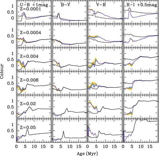
Photometric evolution of colours U − B, B − V, V − R and R − I versus cluster age (in Myr) for Z = 0.0001, 0.0004, 0.004, 0.008, 0.02 and 0.05 from top to bottom panels as labelled. Each colour corresponds to a different cluster mass as in previous figures.
Colours from the clusters without the emission line contamination are plotted with a solid black line. Colours including the contribution of the emission line spectrum are plotted with different colours, according to cluster mass, 0.12, 0.20, 0.40, 0.60, 1.00, 1.50 and 2.00 × 10⁵ M⊙, from the lighter colour (yellow) to the darkest one (purple), using the same coding as in the previous figures. As explained before, a different cluster mass implies not only a variation in the number of ionizing photons but also a change in the size of the associated H ii region due to the assumption (in our models) that the bubble radius depends on the total mechanical energy deposited by the cluster's winds and SNe.
This figure shows that colours have very different values when the emission-line contribution is included in the calculation. These variations in the expected colours for a young stellar cluster are especially important for low-to-intermediate metallicities (Z = 0.0004–0.008); this seems reasonable, as the emission lines in the visible have the strongest intensities in this abundance range.
The contaminated colours U − B and B − V for all metallicities, and all colours for high metallicity (Z > 0.008) evolve with age, reaching the uncontaminated colours as soon as the emission lines disappear near 5.5 Myr (this value depends on the metallicity, as discussed in Paper II). However, V − R and R − I contaminated colours at low metallicity still show variations with respect to the uncontaminated colours even up to ages of ∼20 Myr.
This is because these colours are contaminated by hydrogen emission lines, and the R band is the most highly contaminated. This indicates the presence of ionizing photons – i.e. a young population – which produces Hα emission that falls almost in the centre of the R band, near to the maximum of the filter transmission curve, producing a redder V − R colour simultaneous to a bluer R − I.
We note again that Hα emission is expected even for ages beyond 5.5 Myr (when other emission lines cannot be produced) and is detectable up until ages of 10–20 Myr, depending upon metallicity. Up to now, arguments for a reddened colour had been based upon the claim for an old underlying population or a dust excess. We show here that a reddened V − R colour, with a contemporaneous blue R − I, in an SSP, can be explained in a new way: with the presence of a young population, which possesses sufficient numbers of ionizing photons to produce Hα emission.
In a similar manner, Fig. 10 shows the effect of these emission lines in the SDSS filter system. Differences in colours, with and without the contribution of the emission lines, are even more substantial than in the Johnson system, reaching in some colours, difference of up to one magnitude.
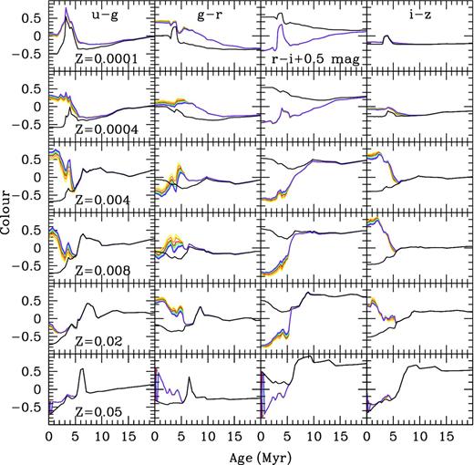
Photometric evolution of colours u − g, g − r, r − i and i − z versus cluster age (in Myr) for Z = 0.0001, 0.0004, 0.004, 0.008, 0.02 and 0.05 from top to bottom panels as labelled. Each colour corresponds to a different cluster mass as in previous figures.
Colour–colour diagrams
Fig. 11 shows four Johnson colour–colour diagrams for SSPs up to 20 Myr in age: U − B versus B − V (top left); B − V versus V − R (top right); B − V versus V − I (bottom left) and V − R versus R − I (bottom right). We show results for Z =0.008, panel (d) and the corresponding ones to other metallicities, Fig. 11(a), (b), (c), (e) and (f) will be in electronic format. Different colours correspond to different cluster masses, as in Fig. 9. Black open ones correspond to the youngest ages including the nebular continuum contribution but not the emission lines.
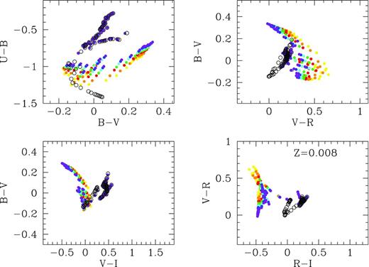
Colour–colour diagrams for young clusters. Panel (d) shows results for Z = 0.008 – top left: U − B versus B − V; top right: B − V versus V − R; bottom left: B − V versus V − I and bottom right: V − R versus R − I. The open and full dots represent the results without and with emission lines. Each colour corresponds to a different cluster mass. The same figures for the other metallicities: Z = 0.0001, 0.0004, 0.004, 0.02 and 0.05, panels (a), (b), (c), (e) and (f) are given in electronic format.
In panels of the U − B versus B − V diagram, we observe that when young stellar populations (contaminated and uncontaminated) colours are plotted, the points fall out of the location expected when standard SSP synthetic colours without the emission line (or continuum) contribution are used. The nebular continuum moves the points out of the standard sequence for old (age ≥ 20 Myr, see Fig. 13) stellar populations. Moreover, when the emission lines contribution is included in the colour calculation, the sequence shows almost the original slope, but moved to an almost parallel line for Z < 0.02, with higher B − V for similar U − B.
Observing the B − V versus V − R diagram, the situation changes, since the contaminated colours fall in the same region of the plot, albeit in an orthogonal sense, in most cases. This behaviour appears independent of the stellar cluster mass, especially for Z = 0.004 and 0.008. This characteristic might allow one to predict the strength of a new starburst overlaid upon an underlying and older stellar population. Further, one might determine the age of this burst from the distance of a given point to the canonical line of old ages. This effect is stronger when mixed population models (Section 4) are interpreted.
In the B − V versus V − I diagrams, the youngest stellar populations show colours with the same trend as the uncontaminated ones for some metallicity cases, while appearing orthogonal for others. On the one hand, the Hα emission reddens the V − I colour. On the other, if the metallicity is intermediate (Z = 0.004–0.008), the oxygen emission lines also increase the luminosity in the V band, since the nebular cooling is mostly done through [O iii] lines. The resulting populated area is very different from the one with uncontaminated SSP colours.
Finally, the V − R versus R − I diagram is the one most affected by the contribution of Hα emission to the R-band luminosity (which dominates the effect of sulphur lines contributing to the I band). This diagram may therefore be useful to check if these contamination effects (due to a young ionizing population) are present regardless of the cluster physical properties, since all the metallicities and cluster mass change the colour–colour diagram with respect to the canonical uncontaminated models. Fig. 12 is similar to Fig. 11 for SDSS colour–colour diagrams.
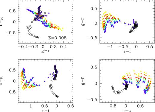
Colour–olour diagrams for young clusters. Panel (d) shows results for Z = 0.008 – top left: u − g versus g − r; top right: g − r versus r − i; bottom left: u − g versus r − i and bottom right: r − i versus i − z. The ppen and full dots represent the results without and with emission lines. Each colour corresponds to a different cluster mass. The same figures for the other metallicities: Z = 0.0001, 0.0004, 0.004, 0.02 and 0.05, panels (a), (b), (c), (e) and (f) are given in electronic format.
In summary, our remarkable conclusions from Figs 11 and 12 are as follows. (1) The youngest stellar population models – therefore, those contaminated most by emission lines – do not follow the generic trend shown by SSP colours calculated in the absence of this emission line contribution, and (2) these young regions’ colours fall in a well-defined region for each colour–colour diagnostic diagram. In some cases (e.g. B − V versus V − R), this region of contaminated colours is located orthogonally to the region where the canonical uncontaminated colours reside. It is clear that emission lines change strongly the location of the models in any given colour–colour diagram. We emphasize that most observers use canonical (uncontaminated and probably without the nebular continuum contribution) models to compare with their star-forming region photometry and use these to derive the properties of the unveiled young stellar population. In some cases, a reddened colour is often interpreted as implying the existence of an old population. As we have demonstrated in the previous paragraphs and shown in the accompanying figures, we can interpret reddening in some colours, instead, actually as a proof of the existence of a young population. In other cases, the lack of good fitting between the classical photometrical models (uncontaminated colours) and the observations is interpreted as extinction (reddened colours are interpreted as dust contamination). This can lead to an overestimation of dust and extinction when this value is derived from photometric data in H ii regions, even after correcting for an underlying old component. In summary, the interpretation has to be done using contaminated models and of course the impact will depend on the colours chosen.
Finally, and as an extension of Figs 11 and 12, we have used all the models together in Fig. 13. This figure shows the eight different colour–colour diagrams (four for Johnson and four for SDSS filters). Models from different metallicities have been plotted together. Large black symbols correspond to the young stellar cluster colours without contamination of emission-line spectra. Coloured symbols correspond to values that include the emission-line contribution for the youngest ages (between 1.0 and 5.0 Myr). Different cluster masses (which, we remind, in our models implies different H ii regions’ inner radii and therefore different emission-line spectrum) have been represented with the same colours as seen previously in Figs 9 and 10. Finally, together with the young clusters, we have included the whole evolutionary sequence, that is, all metallicities in the range Z = 0.0001–0.05 and all ages from 20 Myr up to 15 Gyr, obtained with popstar in Paper I, as grey full dots. This figure shows a clear age sequence for SSP ages older than 10 Myr in all colour–colour diagrams. This sequence places pure young populations (ages below 10–20 Myr) and pure old SSPs in completely different areas in the plot since the youngest fall out of the old sequence. We have plotted a dashed line in each colour–colour diagram to separate the zone where young stellar clusters would reside from the one where the old stellar populations fall. When the young populations with the contaminated colours are included, the diagrams change again since some colours are redder, more similar to the ones of older populations, but others are bluer, and therefore points are located in different diagram regions. The problem is even worse when mixed populations are studied as discussed in Section 4.
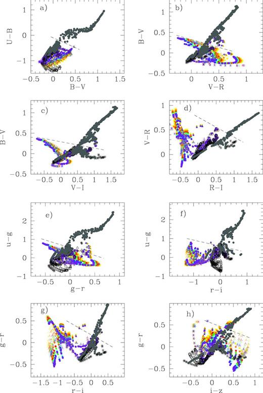
Colour–colour diagrams evolution for all ages and all metallicities. Panels show (a) U − B versus B − V; (b) B − V versus V − R; (c) B − V versus V − I; (d) V − R versus R − I; (e) u − g versus g − r; (f) u − g versus r − i; (g) g − r versus r − i and (h) g − r versus i − z. The dashed black lines separate the old stellar population region (τ > 20 Myr) from the zone of young ones. Colours represent different cluster masses, as in previous figures. The grey full dots correspond to the stellar population colours without any nebular contribution. The black symbols represent colours including the nebular continuum contribution but not the emission lines one. All cluster metallicities and ages have been included in the figure.
Colours versus other photometric parameters
We have used in this work not only the information coming from the colours but also that associated with other photometric parameters. Fig. 14 shows the relationship between colours (both Johnson and SDSS) and equivalent widths of Hα. We have plotted all masses, metallicities and ages together in the same plot.
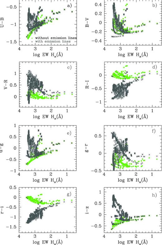
Colours versus log of Hα equivalent width diagrams: (a) U − B versus log EW(Hα) ; (b) B − V versus log EW(Hα); (c) V − R versus log EW(Hα); (d) R − I versus log EW(Hα); (e) u − g versus log EW(Hα); (f) g − r versus log EW(Hα); (g) r − i versus log EW(Hα) and (h) i − z versus log EW(Hα). In all panels full (green), the dots and (black) crosses represent the results without and with emission lines, respectively. All cluster masses, metallicities and ages have been included in the figure.
The original colours without the emission-line contribution are the full green dots. These models define a clear sequence in all plots. Colours including the contribution of emission lines are the black crosses. The equivalent width in this case does not change with the emission lines, while the colours do. This causes the points to move up or down with respect to their original position. Panel (a) shows that in a given time, U − B becomes redder and the points move up slightly. This occurs when EW(Hα) is still quite high (young ages).
The same occurs in panel (c) with V − R, although in this case the reddening extends also for low values of EW(Hα). Changes in panel (b), the B − V colour, are less evident because emission lines contaminate both B and V band in a comparable proportion. Panel (d) shows how the R − I points move down (towards bluer colours), since R is a highly contaminated band. We cannot find a clear metallicity dependence in these plots.
The figure of EW Hα versus U − B is particularly interesting because most of the data cannot be reproduced with pure SSPs as Martín-Manjón et al. (2008, and references therein) showed. The usual explanation was the existence of an underlying older stellar population which, in addition to the recent starburst, could reproduce simultaneously a red U − B colour together with the observed values of the Balmer lines equivalent widths. We claim that, even without adding an old population, an U − B reddening due to the strong contribution of the emission lines in this colour is predicted. The effect is a larger dispersion in the plot, erasing the original trend in the plot U − B colour versus EW(Hα) which showed an age sequence from the high equivalent width and blue colour to the low equivalent width and red colour.
Panels (e)–(h) represent the same kind of plots but for the SDSS colours. A clear separation of the colour sequences without and with emission lines is seen, mainly for the r − i colour, where Hα has a stronger contribution. These plots may be useful to separate young (ages τ < 20 Myr and clear Hα emission) from old stellar populations.
MIXED POPULATIONS
All the models presented in the previous sections assume that there is a single cluster producing the colours of the observed region. In more massive objects where different stellar populations coexist, the contribution of the youngest cluster (responsible for the ionization and the emission lines) mass to the total stellar mass can change the final broad-band magnitudes and therefore the colours. The more massive the young population, the more important the contribution of emission lines to the integrated colours. On the contrary, objects where the young population contribution is small can be well fitted by canonical synthetic colours since the contribution of the emission lines to the total luminosity and therefore to the colours will be minimal.
The calculation of the mixed population (combination of young and old clusters) colours requires a good reference grid of models that allows one to derive the physical properties of composite stellar systems when only photometric information is available. This section is devoted to these composite models in which we have a young ionizing stellar burst superimposed upon an underlying old population. The difference with earlier work in the field (see Paper I for a review of Evolutionary Synthesis Models) is that the emission lines coming from the ionization and the nebular continuum, both produced by the young cluster, are included when computing the integrated colours. We remark the fact that these models have been computed in a consistent manner by taking into account the cluster evolution (and therefore the mechanical energy) to derive the region's photometric size and therefore the radius that, together with the number of ionizing photons and SED shape, determines the ionization parameter responsible for the emission-line luminosities. These emission-line luminosities are the ones included in the colour determination after weighting the luminosities (from both old and young populations) according to their relative masses.
This paper is focused on showing the importance of the emission-line contributions in mixed population colours for nearby H ii and starburst regions at redshift zero. The effect will be similar for more distant galaxies, where the emission-line contribution to the different bands will change with redshift for the standard systems (e.g. Johnson, SDSS, etc.).
This can impact upon estimations of some M/L relationships and/or dust extinction in systems at different redshifts dominated by young ionizing star-forming bursts. It will also be more important at increasing redshift than at redshift zero, since the star formation becomes more violent and the mass of the young ionizing population becomes larger.
When a detailed study of the photometric evolution at high redshift is performed, it will be necessary to take into account that a large number of star-forming regions could be contributing in the different pass-bands, changing the canonical and widely accepted colour–colour theoretical diagrams for synthetic populations. This will be the object of future work in this series.
We have calculated the colours of a system composed of two populations: one older than 100 Myr (logτ ≥ 8.00) and one younger than this same limit (logτ < 8.00). The stellar mass of the young population in this model grid takes the same values as in the SSP models: 0.12, 0.20, 0.40, 0.60, 1.0, 1.5 and 2.0 × 10⁵ M⊙. For each model or composite system, we assume an old stellar population with a mass on the zero-time main sequence defined by a factor F = Mold/Myoung. We have taken six possible values for this grid, F = 0, 1, 10, 100, 1000 and 5000. Colours are computed by using the total luminosity emitted by both the old population and the young stellar population, including the emission-lines contribution and the nebular continuum, as we show in the previous sections.
We have obtained a table for each old stellar population defined by its age and metallicity, where all possible combinations with the young stellar population (scanning the grid in mass, age and metallicity of the young cluster) are included. We show in Table 6 an example of this type of result. The complete set of tables for all ages and metallicities of the old stellar population are available in electronic format (and they are also available at the popstar web page http://www.fractal-es.com/PopStar). Different columns in Table 6 list column 1 and 2, the metallicity and age of the old population; columns 3 and 4, the metallicity and age of the young cluster; column 5, the factor F or mass-ratio between old and young populations; column 6, the young population's mass; column 7, the outer radius (or observed photometrical radius) of the region in pc; column 8, the logarithm of the luminosity of Hα in erg s−1; column 9, the equivalent with of Hα, EW (Hα), in Å; columns 10–14 list the magnitude V and colours U − B, B − V, V − R and R − I, respectively, corresponding to Johnson system, and in which the emission-line contribution has been included, columns 15–19 list the same quantities as in columns 10–14 but without the emission–line contribution (canonical system). Similarly, columns 20–24 list the magnitudes g and colours u − g, g − r, r − i and i − z (of the SDSS system) including the emission-line contribution while columns 25–29 list the same quantities without the emission-line effect.
Example of Johnson and SDSS colour evolution table for two mixed stellar populations. The complete table is in electronic format.
| Zo | logτo | Zy | logτy | F | Mcl | Rout | log LHα | EW Hα | Vc | U − Bc | B − Vc | V − Rc | R − Ic | |
|---|---|---|---|---|---|---|---|---|---|---|---|---|---|---|
| (yr) | (yr) | (M⊙) | (pc) | (ers s− 1) | (Å) | |||||||||
| 0.008 | 8.00 | 0.0001 | 6.00 | 0 | 1.2 × 10⁴ | 126.45 | 38.81 | 1757.00 | −10.315 | −0.850 | −0.011 | 0.736 | −0.549 | |
| 0.008 | 8.00 | 0.0001 | 6.00 | 1 | 1.2 × 10⁴ | 126.45 | 38.81 | 1643.81 | −10.380 | −0.827 | −0.004 | 0.711 | −0.509 | |
| 0.008 | 8.00 | 0.0001 | 6.00 | 10 | 1.2 × 10⁴ | 126.45 | 38.81 | 1030.71 | −10.838 | −0.680 | 0.034 | 0.559 | −0.277 | |
| 0.008 | 8.00 | 0.0001 | 6.00 | 100 | 1.2 × 10⁴ | 126.45 | 38.81 | 172.46 | −12.456 | −0.388 | 0.092 | 0.285 | 0.105 | |
| 0.008 | 8.00 | 0.0001 | 6.00 | 1000 | 1.2 × 10⁴ | 126.45 | 38.81 | −39.88 | −14.810 | −0.290 | 0.108 | 0.202 | 0.214 | |
| 0.008 | 8.00 | 0.0001 | 6.00 | 5000 | 1.2 × 10⁴ | 126.45 | 38.81 | −61.54 | −16.544 | −0.280 | 0.110 | 0.193 | 0.226 | |
| 0.008 | 8.00 | 0.0001 | 6.00 | 0 | 2.0 × 10⁴ | 163.68 | 39.03 | 1757.00 | −10.878 | −0.845 | −0.007 | 0.726 | −0.548 | |
| 0.008 | 8.00 | 0.0001 | 6.00 | 1 | 2.0 × 10⁴ | 163.68 | 39.03 | 1643.60 | −10.943 | −0.822 | −0.001 | 0.701 | −0.508 | |
| 0.008 | 8.00 | 0.0001 | 6.00 | 10 | 2.0 × 10⁴ | 163.68 | 39.03 | 1029.86 | −11.397 | −0.677 | 0.036 | 0.552 | −0.276 | |
| 0.008 | 8.00 | 0.0001 | 6.00 | 100 | 2.0 × 10⁴ | 163.68 | 39.03 | 172.05 | −13.012 | −0.387 | 0.093 | 0.284 | 0.105 | |
| 0.008 | 8.00 | 0.0001 | 6.00 | 1000 | 2.0 × 10⁴ | 163.68 | 39.03 | −39.93 | −15.365 | −0.290 | 0.108 | 0.202 | 0.214 | |
| 0.008 | 8.00 | 0.0001 | 6.00 | 5000 | 2.0 × 10⁴ | 163.68 | 39.03 | −61.55 | −17.099 | −0.280 | 0.110 | 0.193 | 0.226 | |
| −10.076 | −1.245 | 0.158 | 0.253 | 0.152 | −10.124 | −0.010 | 0.424 | −0.890 | −0.167 | −9.619 | −0.499 | 0.009 | 0.030 | −0.228 |
| −10.157 | −1.196 | 0.154 | 0.249 | 0.157 | −10.177 | 0.015 | 0.405 | −0.851 | −0.154 | −9.703 | −0.443 | 0.004 | 0.024 | −0.211 |
| −10.696 | −0.913 | 0.137 | 0.226 | 0.185 | −10.567 | 0.182 | 0.285 | −0.618 | −0.091 | −10.259 | −0.114 | −0.019 | −0.005 | −0.123 |
| −12.425 | −0.437 | 0.115 | 0.198 | 0.220 | −12.077 | 0.550 | 0.040 | −0.199 | −0.011 | −12.008 | 0.485 | −0.049 | −0.042 | −0.017 |
| −14.807 | −0.296 | 0.111 | 0.192 | 0.228 | −14.402 | 0.686 | −0.044 | −0.070 | 0.008 | −14.394 | 0.679 | −0.055 | −0.051 | 0.007 |
| −16.543 | −0.281 | 0.110 | 0.191 | 0.229 | −16.133 | 0.702 | −0.054 | −0.056 | 0.010 | −16.131 | 0.701 | −0.056 | −0.052 | 0.009 |
| −10.631 | −1.245 | 0.158 | 0.253 | 0.152 | −10.687 | −0.001 | 0.414 | −0.888 | −0.168 | −10.174 | −0.499 | 0.009 | 0.030 | −0.228 |
| −10.712 | −1.196 | 0.154 | 0.249 | 0.157 | −10.740 | 0.024 | 0.396 | −0.849 | −0.155 | −10.258 | −0.444 | 0.004 | 0.024 | −0.211 |
| −11.251 | −0.913 | 0.137 | 0.226 | 0.185 | −11.128 | 0.188 | 0.279 | −0.616 | −0.091 | −10.814 | −0.114 | −0.019 | −0.005 | −0.124 |
| −12.980 | −0.437 | 0.115 | 0.198 | 0.220 | −12.633 | 0.552 | 0.038 | −0.199 | −0.011 | −12.563 | 0.485 | −0.049 | −0.042 | −0.017 |
| −15.362 | −0.296 | 0.111 | 0.192 | 0.228 | −14.957 | 0.687 | −0.045 | −0.070 | 0.008 | −14.949 | 0.679 | −0.055 | −0.051 | 0.007 |
| −17.098 | −0.281 | 0.110 | 0.191 | 0.229 | −16.687 | 0.702 | −0.054 | −0.056 | 0.010 | −16.686 | 0.701 | −0.056 | −0.052 | 0.009 |
Colour evolution
Fig. 15 shows two examples of these mixed populations. We show the time evolution of the same colours as in the previous SSP figures for two cases: case (1) in the four top panels, we consider a stellar system composed of an old stellar population of 10 Gyr and Z = 0.0001 plus a young stellar population of 105 M⊙ and Z = 0.0004. The figure shows the colour evolution with the young cluster age, ranging from 0 to 20 Myr. Case (2) in the four bottom panels, we consider the mixing of an old stellar population of 10 Gyr and |$\rm$|Z= 0.004 with a young cluster mass of 105 M⊙ and metallicity of Z = 0.008. In all cases, the dashed lines are the colours calculated without the emission-line contribution, while the solid lines correspond to the total colour including this contribution. Different colours indicate different F values, ranging from 0 (black, meaning a pure young population) to 5000 (red, meaning a quite important mass contribution of the underlying old component, in this case 5 × 10⁸ M⊙ since the young cluster mass is 105 M⊙). These F values and the legend have been labelled in the V − R versus R − I diagrams. The higher the value of F, the smaller the emission lines impact on the integrated colour, as expected. In the plots, larger differences between dashed and solid lines can be appreciated for small F values while both lines are almost coincident for large F values. The cases with F = 0 correspond to a pure young population and therefore to the case discussed in Section 3 of this paper. It can also be seen that as the young population evolves, the contribution of the lines tends to disappear, and the dashed and solid lines tend towards coincidence.
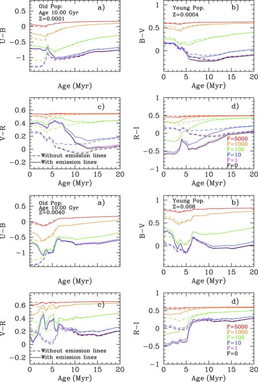
Examples of Johnson colour evolution with a young cluster age in a mixed population. This is composed of an old 10 Gyr underlying cluster plus a young burst (τ < 20 Myr and clear Hα emission). Each colour represents a different mass contribution of the old population to the young burst (F, being mass-old/mass-young) as labelled. Synthetic colours with and without the emission-line contribution are plotted as solid and dashed lines, respectively. Two metallicity cases have been chosen as examples: top panels use Z = 0.0001 and Z = 0.0004 for old and young populations, while bottom panels use Z = 0.004 and Z = 0.008, as labelled in the plots.
When F is in the range 1 (magenta line) to 10 (blue line), the old population contributes in a small proportion and the young population dominates the system. In these cases, colours U − B, V − R and R − I for the first evolutionary phases of the young population (age < 5 Myr) present a behaviour close to the one with F around 100 and no emission-line contribution (green dashed lines). It means that using a mixture of two populations without taking into account the emission-line contribution, can lead to a misinterpretation, by assigning a stronger contribution of the underlying population than the actual one. Thus, for this particular example, the error determination can be as high as one order of magnitude in the F value, implying a similar error for the determination of the mass of the underlying population (assuming that we can constrain the young population mass through other photometric values, like the Hα luminosity).
Only the colour B − V and somehow U − B seem to provide similar estimations for the old population's age, regardless of the models used (with or without emission lines). A similar behaviour is observed in case (2), displayed in the four bottom panels, which indicates that this effect is quite independent of the metallicity for these examples. Of course, these conclusions can change for other combinations of metallicities and for younger ages of the old population. The potential confusion will become larger when a stronger starburst is overlapping with an intermediate-age population. We have plotted this extreme case with a very old underlying population to demonstrate that even in this system we can find important differences in the inferred physical properties when using canonical models instead of the ones with the emission-line contribution.
Fig. 16 shows the same example of mixed populations, but for SDSS colours. The plots for case (1) show the same effect of possible misinterpretation in the colours u − g, g − r and r − i when using uncontaminated colours instead the ones including the emission-line contribution. Again, differences larger than one order of magnitude in the burst strength can be inferred. From the lower panels (case 2), all the colours, and especially r − i and i − z, would lead to misinterpretation. We cannot provide plots for the whole range of age, mass and metallicity of the contributing populations, but given a specific set of photometric observations, a good representation of the reality may be obtained by fitting the different parameters to the theoretical models, following for example a mean square error (MSE) as a measure of estimator quality. We provide the complete set of tables and models in electronic format to allow these computations.
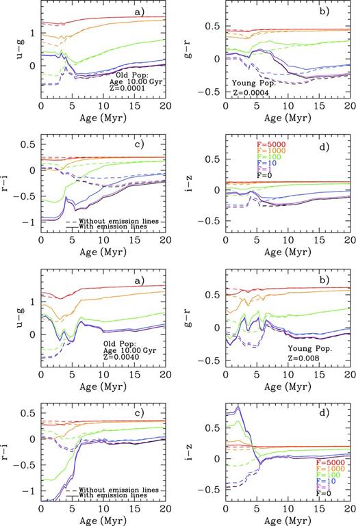
Examples of SDSS colour evolution with a young cluster age for a mixed population. This is composed of an old 10 Gyr underlying cluster plus a young burst (Age τ < 20 Myr and clear Hα emission). Each colour represents a different mass contributions of the old population to the young burst (F, being mass-old/mass-young) as labelled. Synthetic colours with and without the emission-line contribution are plotted as solid and dashed lines, respectively. Two metallicity cases have been chosen as examples: top panels use Z = 0.0001 and Z = 0.0004 for old and young population, while bottom panels use Z = 0.004 and Z = 0.008, as labelled in the plots.
Colour–colour diagrams
The same mix of stellar populations as before are represented in Figs 17 and 18 as colour–colour diagrams. As in Figs 15 and 16, different colour lines represent different ratios in mass, F, between old and young stellar populations. Thus, red lines give the colour–colour results when the old stellar population dominates in mass, with a value of 108 M⊙, the young one of 105 M⊙ while the black lines represent the evolution of a simple young stellar population without underlying population. All the other colours (orange, green, blue and magenta) represent intermediate cases.
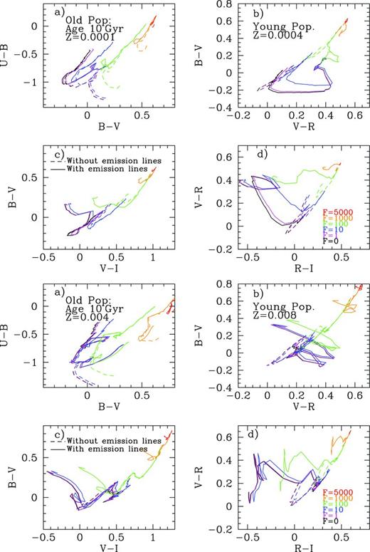
Examples of Johnson colour–colour evolution for a mixed population. This is composed of an old 10 Gyr underlying cluster plus a young burst (τ < 20 Myr and clear Hα emission). Different coloured lines represent a different mass contribution of the old population to the young burst (F, being mass-old/mass-young). Synthetic colours with and without the emission-line contribution are plotted as solid and dashed lines, respectively. Two metallicity cases have been chosen as examples: top panels use Z = 0.0001 and Z = 0.0004 for old and young population respectively while bottom panels use Z = 0.004 and Z = 0.008, as labelled in the plots.
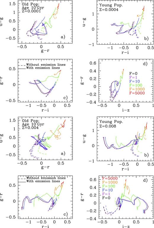
Examples of SDSS colour–colour evolution for a mixed population. This is composed of an old 10 Gyr underlying cluster plus a young burst (τ < 20 Myr and clear Hα emission). Different coloured lines represent a different mass contribution of the old population to the young burst (F, being mass-old/mass-young). Synthetic colours with and without the emission lines contribution are plotted as solid and dashed lines, respectively. Two metallicity cases have been chosen as examples: top panels use Z = 0.0001 and Z = 0.0004 for old and young population, respectively, while bottom panels use Z = 0.004 and Z = 0.008, as labelled in the plots.
The dashed lines are the results without the emission-line contribution while the solid lines show our results including the emission-line contamination. In these figures, the model results given by the solid lines (emission lines included) can be bluer or redder, compared to the models of the dashed lines (no emission lines). This will depend also on F. For a given value of F, models on the solid lines (with lines) will be close or far from the canonical solid line (they can be placed also on an orthogonal line) depending on the age of the young population as discussed in Section 3. Our results predict a large dispersion among the observational values when plotting them in colour–colour plots, explaining in a natural way this fact. Previous work often proposed a reddening excess due to dust to explain the discrepancy between the synthetic colours and the observed ones.
Colours versus Hα equivalent widths
Finally, Figs 19 and 20 show the synthetic colours for the same combinations of stellar populations described in the previous sub-sections versus the equivalent width of Hα with the same meaning of colours and line types for Johnson and SDSS colours, respectively. The emission lines do colours bluer or redder, such as we have seen before, and therefore the resulting solid lines fall in a different region than the dashed lines (canonical models without the emission-line contribution) for a given value of the Hα equivalent width. In the example corresponding to Fig. 19 case 1 (upper panels) B − V (panel b) shows that differences between solid and dashed lines are small, so that estimations based on this type of plot would be similar using the colours with or without emission lines. However, this is not the case for the other colours (panels a, c and d for U − B, V − R and R − I, respectively) for which we suggest that the colours including emission lines are redder (for U − B and V − R) or bluer (for R − I) than the ones synthesized without this contribution. A similar behaviour is found in case 2 (lower four panels).
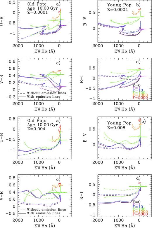
Examples of different Johnson colours – as labelled in the panels – plotted against the equivalent width of Hα in emission for a mixed population. This is composed of an old 10 Gyr underlying cluster plus a young burst (τ < 20 Myr and clear Hα emission). Each coloured line represents a different mass contribution of the old population to the young burst (F, being mass-old/mass-young). Synthetic colours with and without the emission-line contribution are plotted as solid and dashed lines, respectively. Two metallicity cases have been chosen as examples: top panels use Z = 0.0001 and Z = 0.0004 for old and young population, respectively, while bottom panels use Z = 0.004 and Z = 0.008, as labelled in the plots.
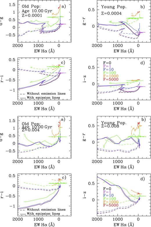
Examples of different SDSS colours – as labelled in the panels – plotted against the equivalent width of Hα in emission for a mixed population. This is composed of an old 10 Gyr underlying cluster plus a young burst (τ < 20 Myr and clear Hα emission). Each coloured line represents a different mass contribution of the old population to the young burst (F, being mass-old/mass-young). Synthetic colours with and without the emission-line contribution are plotted as solid and dashed lines, respectively. Two metallicity cases have been chosen as examples: top panels use Z = 0.0001 and Z = 0.0004 for old and young population, respectively, while bottom panels use Z = 0.004 and Z = 0.008, as labelled in the plots.
As in previous figures, different colour lines correspond to different values of F, from 0 (black, pure young population) to 5000 (red, with a strong mass contribution of the underlying population). For F = 0 models (single population), the evolution shows blue colours and high values of EW(Hα) for the younger clusters, and a progressively decrease of EW(Hα) and colour reddening as far as the cluster evolves. Models on dashed lines do not present simultaneously red colours and high values of EW (Hα) as observed in H ii galaxies for example. This is not the case for the models with the emission lines, in which we can find red colours and high values of EW(Hα) in the range of several hundreds or even few thousands, at early ages, without the need for interpreting this as a dust excess.
Comparison with observational data
In this section, we test our models to see if they can reproduce the photometric observations from star-forming regions where it is already proved that at least a young and an old stellar population exists there. We have analysed the H ii region data of Martínez-Delgado (2009), where photometry exists for a well-observed sample of Blue Compact Dwarf galaxies with spectroscopic metallicity determinations. This makes the sample suitable to compare with our models, in order to see if our predicted colours for mixed populations can reproduce these data. We have plotted different synthetic photometric parameters versus the equivalent width of Hα, which is a proxy of the age, together with observations of H ii regions for two galaxies: III Zw 107 and III Zw 102 in Figs 21 and 22, respectively. In both figures panels (a)–(d) plot the synthetic colours U − B, B − V, V − R and R − I, respectively. Panel (e) uses the Hα luminosity and panel (f) the photometric radius of the H ii region, Rout.
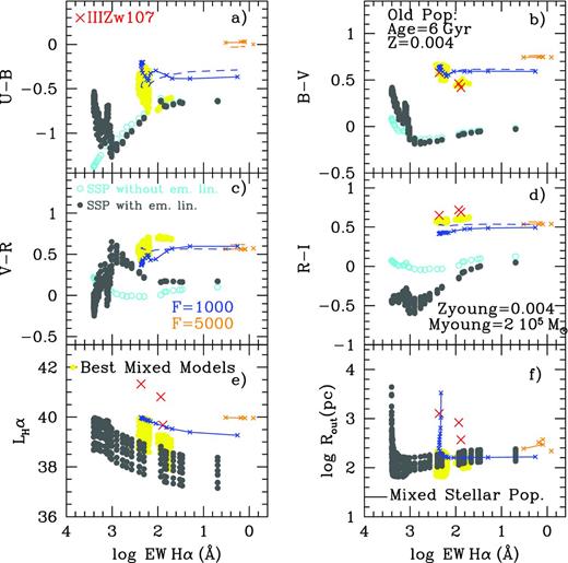
Colours U − B, B − V, V − R and R − I, logarithm of Hα luminosity (erg s−1) and logarithm of the H ii region radius, Rout( in pc), versus EW(Hα). Observed data for star-forming regions in the galaxy III Zw 107 (Martínez-Delgado 2009) are plotted as red crosses. SSPs models with Z = 0.004 are shown with open (cyan) and full (black) dots. The yellow region is the locus of models with Zyoung = 0.004, the estimated metallicity from visible spectroscopy of the observed star-forming regions that are able to reproduce simultaneously the observed colours and EW(Hα). From these two-population mixed models, we have selected those ones with an old population of the same metallicity, Z = 0.004, and 6 Gyr old and two values of F, F = 1000, whose evolution with the young population age is plotted as a blue line, and F = 5000, plotted as an orange line, to show as example the evolution of a mixed population.
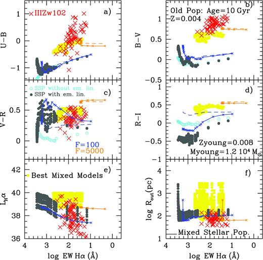
Colours U − B, B − V, V − R and R − I, logarithm of Hαluminosity (in erg s−1) and logarithm of the H ii region radius, Rout( in pc), versus EW(Hα). Observed data for star-forming regions in the galaxy III Zw 102 (Martínez-Delgado 2009) are plotted as red crosses. SSPs models with Z = 0.008 are shown with open (cyan) and full (black) dots. The yellow region is the locus of models with Zyoung = 0.008, the estimated metallicity from visible spectroscopy of the observed star-forming regions that are able to reproduce simultaneously the observed colours and EW(Hα). From the two-population mixed models, we have selected those ones with an old population of Z = 0.004 and 10 Gyr old and two values of F, F = 100, whose evolution with the young population age is plotted as a blue line and F = 5000, plotted as an orange line, to show as example the evolution of a mixed population.
Observed regions in Figs 21 and 22 correspond to data for the galaxies III Zw 107, and III Zw 102, respectively, plotted as red crosses. The metallicity for the first galaxy estimated from its oxygen abundance (itself derived using optical emission lines) is 12 + log [O/H] = 8.23, equivalent to Z ∼ 0.004 (López-Sánchez & Esteban 2010). This metallicity is also consistent with the appearance of WR features in spectroscopy observations. Similarly for III Zw 102, the estimated abundance (from spectroscopic oxygen abundances from 3D spectroscopy) is 12 + log [O/H] = 8.49 (Cairós et al. 2012), equivalent to Z ∼ 0.008.1
In these two galaxies used as examples, it is impossible to explain the observed colours without the existence of an older underlying stellar population, as can be seen in Figs 21 and 22, where the synthetic colours for the case of an SSP (F = 0) of a metallicity as the one estimated from the emission lines as given before, without the contribution of the emission lines (cyan open dots) and with the emission lines (black full dots), cannot reproduce the observed colours. We can see that neither of the two set of models can reproduce the observations. In Figs 21 and 22, we cannot find any solution for colours U − B (panel a), B − V (panel b), V − R (panel c) and R − I (panel d), when data are available, and neither is it possible to find a population able to simultaneously fit the colours and the Hα equivalent width.
The presence of such an underlying old population is widely accepted in BCGs, as the case of III Zw 107 and III Zw 102. Although their low metallicity and the very young stellar populations led some time ago to the proposal that these systems could be suffering their first burst of star formation (Sargent & Searle 1970) more recent observations point to these galaxies seem to be not as young as it was originally thought. Photometric observations indicate that they host stellar populations, reaching in some cases a few Gyr (Telles, Melnick & Terlevich 1997; Legrand 2000; Cairós et al. 2003; Tolstoy 2003; van Zee, Barton & Skillman 2004; Thuan & Izotov 2005). There is now wide agreement about the existence of underlying populations with ages of several Gyr in BCGs and/or H ii galaxies. Even the most metal-poor galaxy known, I Zw18, the best candidate to primordial galaxy, has started forming stars earlier than ∼1 Gyr old (Annibali et al. 2013). For this reason, the fit of a mixed population to the observed data, might improve the result.
Therefore, we have selected among all the mixed stellar populations models computed in our grid and described in the previous section, those ones whose colours and equivalent width EW(Hα) can fit the observations within the error bars. To do that we have performed a chi-square fit of our mixed models in which the metallicity of the young stellar population, Zyoung, is equal to the estimated one by the emission lines as given before. The yellow region in each figure shows the results of this fit. These results represent all possible combinations of Zold+Age-old+Age-young able to reproduce the data within errors. It is clear that there are solutions to the data.
As an example, we also plot in Fig. 21 the evolution with the age of the young population for one of these combinations or mixed stellar populations, which has a young stellar mass of 2 × 10⁵ M⊙, and Z = 0.004 with one 6 Gyr old with Z = 0.004 and with two possible values for mass contributions: F = 1000 (dark blue lines) and F = 5000 (orange lines). Solid lines represent models including emission lines while dashed lines represent models without this contribution. We see that the three observed regions are better fit by the model with F = 1000. In panels (e) and (f), we show the same yellow region. Panel (e) shows that two of the observed regions have Hα luminosities larger than those of the plotted models. This is likely due to the fact that our grid does not include cluster masses larger than 2 × 10⁵ M⊙. At least (although obviously the interpretation would be different if other IMF is used) we can put a lower limit for the mass of these H ii regions.
Similar to Fig. 21, we have plotted Fig. 22 with our models and observed data of star-forming regions in III Zw 102. Again, most of observational points cannot be fit by the SSP. We represent the region of selected mixed models as yellow points as before. This region is not valid for all data and some observed parameters are not reproduced with our current set of models. Perhaps larger F factors are necessary to fit these very red colours in regions where EW(Hα) is still present, or maybe the averaged abundance Z = 0.008 is not representative for all H ii regions. Following the results of panel (e), the young stellar population mass of these regions should be smaller than our lowest limit, 104 M⊙. This would also explain the values of the observed radii also being smaller than the predicted ones. It is necessary to remain that the chi-square fit is performed using only the data of panels (a)–(d), not (e) nor (f). Nevertheless, the two-population mixed model is also a simplification since some of the regions are not spatially resolved and can contain more than two stellar populations with different ages. It has to be noticed that the worse fitting found in the colours U − B and B − V is fully consistent with the strong dust absorption found in this galaxy, as reported by Cairós et al. (2012)
Figs 21 and 22 show that our models can fit real data of photometric observations of H ii regions, obtaining the metallicity and the age for both the young and the old populations and reproducing several colours simultaneously when SSPs cannot do it. Moreover, the inclusion of emission lines in the models is needed to reproduce simultaneously all the colours in the two selected galaxies. It has to be noticed that the two galaxies have very different values of the metallicity, which has been spectroscopically confirmed by different papers in the literature.
Finally, we plot in Fig. 23 data obtained by Mayya (1994) for a sample of H ii regions in external galaxies. Each galaxy's regions are plotted with a different code as labelled in panel (b). Only two colours and the equivalent width EW(Hα) are available for this sample. In this figure, we plot as an example the model with Z = 0.02 for the young stellar population and Z = 0.004 for the old one, with an age of 10 Gyr. Different factors F are shown with lines of different colours as labelled in the plot. We see that most of data could need values of F in the range 100–1000, with only some exceptional points out of the region defined by these two lines. We might perform a similar selection technique to see which models are the best ones to fit these data, or use an MSE analysis to derive the most appropriate models for each galaxy or H ii region, but this is beyond the scope of this work. What we want to show with this figure is that mixed population models including emission lines can reproduce the observations of star-forming regions, while SSPs cannot, and models without emission lines do not offer the same result, and ultimately result in a misinterpretation of the physical stellar population parameters.
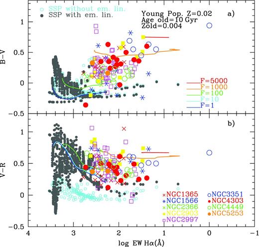
Colours B − V and V − R versus EW(Hα). Observed data are from Mayya (1994) for H ii regions located in different galaxies as labelled in the lower plot. Two mixed populations, an old one with Z = 0.004 and 10 Gyr old and another younger one with Z = 0.02, and different ages over the evolutionary sequence, are represented as solid lines with different colours following the value of F as labelled in the upper diagram. We can see that models could reproduce the observations.
CONCLUSIONS
We have calculated the same grid of magnitudes and colours as in Paper I with the popstar code, but now incorporating the contribution from emission lines, using for that the intensities obtained in our Paper II, for a large grid of young stellar ionizing clusters. We provide tables with uncontaminated and contaminated colours.
Broad-band filter magnitudes are contaminated by the emission lines coming from ionizing nebulae surrounding young stellar clusters. This contamination modifies the magnitudes (ranging from 0.2 to 1.5 mag depending on the filter) in the visible and near-IR bands. Colours U − B, B − V, V − R and R − I are modified by a value between 0.2 and 0.8 mag depending on the colour and the metallicity of the stellar population. Similar results are found in SDSS filters and should be found in other photometric systems.
The synthetic contaminated colours for SSPs in the colour–colour diagrams fall outside the standard canonical sequence shown by the uncontaminated colours or those obtained for old stellar populations. In many cases, they show orthogonal sequences to those ones.
We have also computed other photometric parameters, such as Hα and Hβ luminosities, equivalent widths of Hα and Hβ and radii of the corresponding H ii regions.
The equivalent widths for Hα and Hβ do not depend only on the age. They also depend on the metallicity of the stellar population. The EW(Hα) decreases with age until 5–7 Myr if Z > 0.004. For lower metallicities, EWHα maintains positive values until 15–18 Myr. The same occurs with Hα and Hβ luminosities, which have high values until ∼20 Myr for the lowest metallicities (Z < 0.004).
The outer calculated radii of low-metal H ii regions are quite large compared with those observed at intermediate metallicities. Since these regions are not present in the observational samples, and taking into account that they must show high Hα luminosities too, we need to consider the impact of observational selection effects that might be able to lead the production of biased H ii region samples.
An evolutionary track in the plane Rout-L(Hα) shows that the radius of the region increases when the Hα luminosity decreases. However, a positive correlation L(Hα)-Rout arises when all stellar cluster masses and metallicities are drawn together, so the observed correlation and its dispersion may be explained by a mix of stellar clusters of different ages, metallicities and masses.
We have also computed a grid of models where a recent ionizing burst is mixed with an underlying and older host stellar population in different proportions. We give magnitudes and colours for these mixed stellar populations. In some cases contaminated colours with a low contribution of an old stellar population are similar to the uncontaminated colours with a high proportion of old population. This is important when interpreting observations from regions where there exists an underlying stellar population, since the wrong ratio F will be estimated if the uncontaminated colours, instead the ones contaminated by emission lines, are used when comparing observational data and models to derive physical properties of the stellar populations.
Other photometric parameters have also been given for each mix of stellar populations as before: Hα and Hβ luminosities, equivalent widths for Hα and Hβ and radii of the corresponding H ii regions. This allows one to compare the observed radii of H ii regions, their colours and their equivalent widths of Hα with the models. We have checked with some test cases that our models can reproduce photometric observational data and that it is possible to find the best mix of stellar populations able to fit simultaneously several photometrical observations.
All these models have been computed at redshift zero but detailed models will be available soon for higher redshifts, taking into account their shift with z and the contribution to the different standard filters in the visible and near-IR.
This work has been partially supported by FRACTAL SLNE, DGICYT grant AYA2007-67965-C03-02, AYA2010-21887-C04-02 and AYA2010-21887-C04-03, and partially funded by the Spanish MEC under the Consolider-Ingenio 2010 Program grant CSD2006-00070: First Science with the GTC (http://www.iac.es/consolider-ingenio-gtc/). Also, partial support from the Comunidad de Madrid under grant CAM S2009/ESP-1496 (AstroMadrid) is grateful. An anonymous referee is acknowledged for his or her useful comments that improved this work. We would like to thank Dr B. K. Gibson warmly for his help reviewing this manuscript and correcting the English version.
Solar abundance is taken as: 12 + log [O/H] = 8.67, equivalent to Z = 0.015, (Asplund et al. 2009).
REFERENCES
SUPPORTING INFORMATION
Additional Supporting Information may be found in the online version of this article:
Table 1. Computed radii for the modelled stellar clusters of all ages and metallicities and for ne = 10 and 100 cm−3.
Table 2. Transmission value T of Johnson and SDSS filters.
Table 4. Johnson colours evolution results for the modelled stellar clusters of all ages and metallicities and for ne = 10 and 100 cm−3.
Table 5. SDSS colour evolution results for the modelled SSP of all ages and metallicities and for ne = 10 and 100 cm−3.
Table 6. Johnson and SDSS colour evolution. Complete table for two mixed stellar populations (Supplementary Data).
Please note: Oxford University Press are not responsible for the content or functionality of any supporting materials supplied by the authors. Any queries (other than missing material) should be directed to the corresponding author for the article.
