Dissipation in relativistic superfluid neutron stars

Gusakov, M. E.; Kantor, E. M.; Chugunov, A. I.; Gualtieri, L.

doi:10.1093/mnras/sts129

Abstract

We analyse damping of oscillations of general relativistic superfluid neutron stars. To this aim we extend the method of decoupling of superfluid and normal oscillation modes first suggested in Gusakov & Kantor. All calculations are made self-consistently within the finite temperature superfluid hydrodynamics. The general analytic formulas are derived for damping times due to the shear and bulk viscosities. These formulas describe both normal and superfluid neutron stars and are valid for oscillation modes of arbitrary multipolarity. We show that (i) use of the ordinary one-fluid hydrodynamics is a good approximation, for most of the stellar temperatures, if one is interested in calculation of the damping times of normal f modes, (ii) for radial and p modes such an approximation is poor and (iii) the temperature dependence of damping times undergoes a set of rapid changes associated with resonance coupling of neighbouring oscillation modes. The latter effect can substantially accelerate viscous damping of normal modes in certain stages of neutron-star thermal evolution.

stars: interiors, stars: neutron, stars: oscillations

1 INTRODUCTION

Neutron stars (NSs) are compact objects with the mass M ∼ M_⊙, circumferential radius R ∼ 10 km and the central density ρ_c several times higher than the nuclear density ρ₀ ≈ 2.8 × 10¹⁴ g cm⁻³. They are interesting because of extreme conditions in their interiors and a wide variety of associated astrophysical phenomena. In particular, internal instabilities or external perturbations can excite NS oscillations, which are potentially detectable by the next-generation gravitational wave interferometers (see e.g. Andersson & Kokkotas 2001; Andersson 2003; Owen 2010). It is very probable that quasi-periodic oscillations of electromagnetic radiation observed in the tails of the giant gamma-ray flares are connected with oscillations in NS crust (e.g. Israel et al. 2005; Strohmayer & Watts 2005, 2006; Watts & Strohmayer 2007), and that seismology would become a significant source of information about NSs in the nearest future (Abbot et al. 2007; Andersson et al. 2011; Watts 2011).

For the correct interpretation of already existing and future observations one requires a well-developed theory of oscillating NSs. It should, in particular, (i) be based on the general relativity theory, since NSs are relativistic objects; (ii) employ an adequate model of superdense matter, including realistic equation of state and parameters of baryon superfluidity; and (iii) correctly account for the effects of baryon superfluidity on the hydrodynamics of NS matter.

Let us discuss briefly a (key) role of superfluidity. According to numerous microscopic calculations (see e.g. Lombardo & Schulze 2001), baryon matter in the internal layers of NSs becomes super-fluid at T ≲ 10⁸–10¹⁰ K. It is very difficult to interpret the observa-tional data on pulsar glitches (see e.g. Chamel & Haensel 2008) and cooling of NSs (Yakovlev, Levenfish & Shibanov 1999; Yakovlev & Pethick 2004) without invoking baryon superfluidity. Recent real-time observations of cooling NS in Cassiopea A supernova remnant (Heinke & Ho 2010) also present a strong argument in favour of the existence of baryon superfluidity in the NS core. The observations were explained by Shternin et al. (2011) and Page et al. (2011) within a scenario, suggested for the first time in Gusakov et al. (2004) and Page et al. (2004), and assuming mild neutron superfluidity (with maximum neutron critical temperatures T_cn max ∼ 7-9 × 10⁸ K) and strong proton superconductivity (with maximum proton critical temperatures T_cp max ≳ 2-3 × 10⁹ K) in the NS core.

Combined analysis of all the three factors (i)–(iii) is a formidable task for the oscillation theory so in the literature they were considered successively. The foundations of the relativistic theory of stellar oscillations were laid 50 yr ago by Chandrasekhar (1964) and Thorne & Campolattaro (1967) and were further developed in many subsequent papers (see e.g. Detweiler & Ipser 1973; Ipser & Thorne 1973; Lindblom & Detweiler 1983; Detweiler & Lindblom 1985; Cutler & Lindblom 1987; Cutler, Lindblom & Splinter 1990; Chandrasekhar & Ferrari 1991; Kokkotas & Schutz 1992; Yoshida & Lee 2003a; Lin, Andersson & Comer 2008 and a review of Kokkotas & Schmidt 1999). When studying oscillations of NSs, most of these works considered ordinary one-fluid relativistic hydrodynamics.

Meanwhile it is well known that superfluidity leads to appearance of additional velocity fields, describing the superfluid degrees of freedom (e.g. Khalatnikov & Lebedev 1982; Khalatnikov 1989; Carter & Khalatnikov 1992). This substantially complicates the hydrodynamics of NS matter, making it multifluid (Mendell 1991a,b; Gusakov & Andersson 2006). In addition, superfluidity affects the kinetic coefficients (such as bulk and shear viscosities) and also requires additional viscous coefficients to be introduced (see Gusakov 2007; Gusakov & Kantor 2008 for details).

Oscillations of superfluid NSs have been studied actively only in the last two decades (see e.g. Lee 1995; Lindblom & Mendell 2000; Prix & Rieutord 2002; Yoshida & Lee 2003b; Prix, Comer & Andersson 2004; Samuelsson & Andersson 2009; Wong, Lin & Leung 2009; Passamonti & Andersson 2011, 2012), starting from the pioneering papers by Epstein (1988) and Lindblom & Mendell (1994). However, most of these works neglect general relativity effects and employ zero temperature (T = 0) limit of superfluid hydrodynamics (i.e. hydrodynamics, applicable only at T = 0). Within the general relativity theory oscillations were discussed only by Comer, Langlois & Lin (1999), Andersson, Comer & Langlois (2002), Yoshida & Lee (2003a), Gusakov & Andersson (2006), Lin et al. (2008), Kantor & Gusakov (2011) and Chugunov & Gusakov (2011), but most of these works used zero temperature hydrodynamics. Moreover, in some of these papers (e.g. Andersson et al. 2002; Lin et al. 2008) the presence of superfluid component was modelled by an artificial (polytropic) equation of state which does not represent any specific microphysical model.

Only in the recent papers (Gusakov & Andersson 2006; Chugunov & Gusakov 2011; Kantor & Gusakov 2011) an attempt was made to self-consistently calculate the oscillation spectra using a realistic model of superdense matter and allowing for the effects of finite stellar temperatures. It was shown that in many cases an approximation T = 0 is not justified and, moreover, it can lead to qualitatively incorrect results (Chugunov & Gusakov 2011; Kantor & Gusakov 2011).

Of particular interest is the question of how superfluidity influences dissipation of NS oscillations. It is of extreme importance, for instance, for understanding physical conditions under which a rotating NS becomes unstable with respect to excitation of various oscillations (e.g. r modes), and for estimating gravitational radiation from such stars (e.g. Andersson & Kokkotas 2001).

There were several serious and successful attempts to allow for the effects of superfluidity when studying the dissipation of oscillations in NSs (see e.g. Lindblom & Mendell 1995, 2000; Lee & Yoshida 2003; Andersson, Glampedakis &Haskell 2009; Haskell, Andersson & Passamonti 2009; Haskell & Andersson 2010; Passamonti & Glampedakis 2012), but all of them considered Newtonian stars and used the T = 0 superfluid hydrodynamics. The self-consistent analysis of dissipation in superfluid NSs was only recently performed for a simple case of a radially oscillating NS (Kantor & Gusakov 2011).

The aim of this paper is to fill this gap and to consider, for the first time, dissipation of non-radial oscillations in general relativistic superfluid NSs employing realistic microphysics input with accurate treatment of the effects of finite stellar temperatures.

The paper is organized as follows. Relativistic superfluid hydrodynamics is briefly reviewed in Section 2. Section 3 discusses an unperturbed star and introduces variables describing small deviations of NS from equilibrium. In Section 4 we derive expressions for the oscillation energy and its dissipation rates due to bulk and shear viscosities. In Section 5 the equations that govern oscillations of superfluid NSs are explicitly written out. Section 6 describes the approach to study dissipation of superfluid NS oscillations. This approach is applied for a detailed numerical analysis of realistic models of oscillating NSs in Section 7. Section 8 presents a summary of our results.

In what follows, we use the system of units in which c = k_B = 1, where c is the speed of light and k_B is the Boltzmann constant.

2 DISSIPATIVE SUPERFLUID HYDRODYNAMICS

In this paper we consider, for simplicity, npe matter in NS cores, which is matter composed of neutrons (n), protons (p) and electrons (e). Because both protons and neutrons can be in the superfluid state, one has to use the relativistic hydrodynamics of superfluid mixtures to study oscillations of NSs. Here we briefly discuss the corresponding equations to establish notations and to make the presentation more self-contained. Our consideration closely follows the papers by Gusakov & Andersson (2006), Gusakov (2007) and, especially, Kantor & Gusakov (2011). The reader is referred to these works for more details.

The main distinctive feature of superfluid hydrodynamics is the presence of several velocity fields in the mixture. In our case, these are the four-velocity u^μ of the ‘normal’ (non-superfluid) component of matter (electrons and Bogoliubov excitations of neutrons and protons) as well as the ‘four-velocities’ of superfluid neutrons v^μ_s(n) and superfluid protons v^μ_s(p). In what follows instead of the velocities v^μ_s(n) and v^μ_s(p) it will be convenient to use the four-vectors w^μ_(i) = μ_i[v^μ_s(i) − u^μ], where μ_i is the relativistic chemical potential for particle species i = n or p. A presence of several velocity fields modifies the expressions for the current densities of neutrons j^μ_(n) and protons j^μ_(p),

\begin{equation} j^{\mu }_{(i)} = n_i u^{\mu } + Y_{ik} w^{\mu }_{(k)} \end{equation}

(1)

in comparison with the standard expression j^μ_(i) = n_iu^μ. The electron current density j^μ_(e) has a standard form

\begin{equation} j^{\mu }_{({ {\rm e}})} = n_{\rm e} u^{\mu }. \end{equation}

(2)

Here and below the subscripts i and k refer to nucleons: i, k = n, p; n_l is the number density of particle species l = n, p and e. Unless otherwise stated the summation is assumed over the repeated nucleon indices i, k and over the spacetime indices μ, ν, … (Greek letters). In equation (1) Y_ik is the relativistic entrainment matrix, which is a generalization of the concept of superfluid density (see e.g. Khalatnikov 1989) to the case of relativistic mixtures. In the non-relativistic theory, a similar matrix was first considered by Andreev & Bashkin (1975). The matrix Y_ik is symmetric, Y_ik = Y_ki, and is expressed in terms of the Landau parameters F^ik₁ of asymmetric nuclear matter and universal functions of temperature, Φ_i, as described in Gusakov, Kantor & Haensel (2009b). In beta-equilibrium it can be presented as a function of density ρ and the combinations T/T_cn and T/T_cp: Y_ik = Y_ik(ρ, T/T_cn, T/T_cp), where T is the temperature, T_cn(ρ) and T_cp(ρ) are the density-dependent neutron and proton critical temperatures, respectively. If, for example, T > T_cn then all neutrons are normal. The important property of the matrix Y_ik is that for any non-superfluid species l = n or p, the corresponding elements Y_lk of this matrix vanish.

In this paper we consider NS oscillations, whose frequencies are well below the electron and proton plasma frequencies. In that case the quasi-neutrality condition, n_e = n_p, should hold in an oscillating star, from which it follows (for a non-rotating non-magnetized NS) j^μ_(p) = j^μ_(e) or, in view of equations (1) and (2),

\begin{equation} Y_{pk} w^{\mu }_{(k)}=0. \end{equation}

(3)

Below we assume that this condition is always satisfied. It relates the four-vectors w^μ_(n) and w^μ_(p).

In what follows, along with u^μ and w^μ_(i) it will be convenient to introduce the quantity X^μ, describing superfluid degrees of freedom, as well as the quantity which we call the ‘baryon four-velocity’ U^μ_(b) (note, however, that it is not a four-velocity in the usual sense, because generally U^μ_(b)U_(b) μ ≠ −1, see equation 45 and the footnote ⁴). They are defined by the formulas

\begin{eqnarray} X^{\mu } &=& \frac{Y_{{\rm n}k} w^{\mu }_{(k)}}{n_{\rm b}}, \end{eqnarray}

(4)

\begin{eqnarray} U^\mu _{({\rm b})} &=& u^{\mu }+X^{\mu }, \end{eqnarray}

(5)

where n_b = n_n + n_p is the baryon number density. Note that, as follows from equations (1)–(3), the baryon current density j^μ_(b) = j^μ_(n) + j^μ_(p) is related to U^μ_(b) by the standard equation,

\begin{equation} j^{\mu }_{({\rm b})}=n_{\rm b} \, U^{\mu }_{({\rm b})}, \end{equation}

(6)

while j^μ_(e) equals

\begin{equation} j^{\mu }_{\rm (e)}=n_{\rm e} \left[U_{({\rm b})}^{\mu } - X^{\mu } \right]. \end{equation}

(7)

Together with the quasi-neutrality condition (n_e = n_p) and equation (3), the equations of superfluid hydrodynamics include (Gusakov 2007) the following.

Continuity equations for baryons (b) and electrons (e):
\begin{eqnarray} j^{\mu }_{ ({\rm b}) ; \, \mu } &=& 0, \end{eqnarray}
(8)
\begin{eqnarray} j^{\mu }_{({\rm e}) ; \, \mu } &=& 0. \end{eqnarray}
(9)
Energy–momentum conservation:
\begin{eqnarray} T^{\mu \nu }_{; \,\mu } &=& 0, \end{eqnarray}
(10)
\begin{eqnarray} T^{\mu \nu } &=& (P+\varepsilon ) \, u^{\mu } u^{\nu } + P g^{\mu \nu } + Y_{ik} \left( w^{\mu }_{(i)} w^{\nu }_{(k)} + \mu _i \, w^{\mu }_{(k)} u^{\nu }\right.\nonumber\\[5pt] &&\left. + \mu _k \, w^{\nu }_{(i)} u^{\mu } \right)+\tau ^{\mu \nu }, \end{eqnarray}
(11)
\begin{eqnarray} \tau ^{\mu \nu } &=& - \eta \, H^{\mu \gamma } \, H^{\nu \delta } \,\, \left( u_{\gamma ; \delta } + u_{\delta ; \gamma } - {2 \over 3} \,\, g_{\gamma \delta } \,\, u^{\varepsilon }_{;\varepsilon } \right)\nonumber\\ && - \xi _{1 {\rm n}} \, H^{\mu \nu } \, \left[ Y_{{\rm n} k} w^{\gamma }_{(k)} \right]_{; \gamma } - \xi _2 \, H^{\mu \nu } \, u^{\gamma }_{;\gamma }. \end{eqnarray}
(12)
Potentiality condition for superfluid motion of neutrons:
\begin{eqnarray} \mathrm{\partial} _{\nu } \left[ w_{({\rm n}) \mu } + (\mu _{\rm n} + \varkappa _{\rm n}) u_{\mu } \right] &=& \mathrm{\partial} _{\mu } \left[ w_{({\rm n}) \nu } +(\mu _{\rm n} + \varkappa _{\rm n}) u_{\nu } \right], \end{eqnarray}
(13)
\begin{eqnarray} \varkappa _{\rm n} &=& - \xi _{3{{\rm n}}} \, \left[ Y_{{\rm n}k} w^{\mu }_{(k)} \right]_{;\mu } - \xi _{4{\rm n}} \, u^{\mu }_{;\mu }. \end{eqnarray}
(14)
(iv) The second law of thermodynamics:
\begin{equation} {\rm d} \varepsilon = T \, {\rm d} S + \mu _{\rm e} \, {\rm d} n_{\rm e} + \mu _i \, {\rm d} n_i + \frac{Y_{ik}}{2} \, {\rm d} \left[w^{\alpha }_{(i)} w_{(k) \alpha } \right]. \end{equation}
(15)
In formulas (8)–(15) g^μν is the metric tensor; H^μν ≡ g^μν + u^μu^ν; ∂_μ ≡ ∂/(∂x^μ); P, ε, S and μ_e are the pressure, energy density, entropy density and relativistic electron chemical potential, respectively. These quantities are related by the formula:
\begin{equation} P=-\varepsilon + \mu _{\rm e} n_{\rm e} + \mu _i n_i + {\it TS}. \end{equation}
(16)
Finally, η is the shear viscosity coefficient and ξ_1n, ξ₂, ξ_3n and ξ_4n are the bulk viscosity coefficients. Because of the Onsager symmetry principle, one has
\begin{equation} \xi _{1{\rm n}}=\xi _{4{\rm n}}. \end{equation}
(17)
Moreover, if the bulk viscosities are generated solely by the direct or modified URCA processes, one has an additional constraint (Gusakov 2007)
\begin{equation} \xi _{1{\rm n}}^2=\xi _2 \xi _{3{\rm n}}. \end{equation}
(18)
In the absence of superfluidity the only non-zero coefficient is ξ₂ – the ordinary bulk viscosity.

To close the system describing superfluid hydrodynamics one should put two additional constraints on the four-vectors u^μ and w^μ_(n):

\begin{eqnarray} u_{\mu }u^{\mu }&=&-1, \end{eqnarray}

(19)

\begin{eqnarray} u_{\mu } w^{\mu }_{({\rm n})}&=&0. \end{eqnarray}

(20)

The first constraint is the standard normalization condition while the second one indicates that the comoving frame, in which we measure various thermodynamic quantities (e.g. n_i, ε, …), is defined by the condition u^μ = (1, 0, 0, 0) (Gusakov & Andersson 2006; Gusakov 2007). Using equations (1), (11), (12), (19) and (20) one then immediately finds that n_l = −u_μj^μ_(l) (l = n, p, e) and ε = u_μu_νT^μν.

Making use of the hydrodynamics described above, one can derive the entropy generation equation, valid for superfluid matter. Following the derivation of the similar equation (33) in Gusakov (2007), one arrives at

\begin{equation} S^{\mu }_{;\mu } = - {\varkappa _{\rm n} \over T} \,\, \left[ Y_{{\rm n}k} w^{\mu }_{(k)} \right]_{;\mu } -\tau ^{\mu \nu } \,\, \left( {u_{\nu } \over T} \right)_{;\mu }, \end{equation}

(21)

where the entropy density current S^μ is¹

\begin{equation} S^{\mu } = S u^{\mu } - {u_{\nu } \over T} \,\, \tau ^{\mu \nu }. \end{equation}

(22)

When writing equation (21) we neglected small dissipative terms, as it is discussed in Gusakov (2007). Introducing

\begin{eqnarray} Q_{\rm bulk} &\equiv & \left\lbrace \sqrt{\xi _{3{\rm n}}} \,\,\left[Y_{{\rm n}k} w^{\mu }_{(k)}\right]_{;\mu } +\sqrt{\xi _2} \,\, u^{\mu }_{;\mu } \right\rbrace ^2, \end{eqnarray}

(23)

\begin{eqnarray} Q_{\rm shear} &\equiv& \eta \, H^{\mu \gamma } \, H^{\nu \delta } \,\, \left( u_{\gamma ; \delta } + u_{\delta ; \gamma } - {2 \over 3} \,\, g_{\gamma \delta } \,\, u^{\varepsilon }_{;\varepsilon } \right) u_{\nu ;\mu } \nonumber \\ &=& \frac{\eta }{2} \, H^{\mu \gamma } \, H^{\nu \delta } \left( u_{\gamma ; \delta } + u_{\delta ; \gamma } - {2 \over 3} \,\, g_{\gamma \delta } \,\, u^{\varepsilon }_{;\varepsilon } \right) \nonumber\\ && \times \; \left( u_{\nu ; \mu } + u_{\mu ; \nu } - {2 \over 3} \,\, g_{\mu \nu } \,\, u^{\varepsilon }_{;\varepsilon } \right), \end{eqnarray}

(24)

equation (21) can be rewritten as

\begin{equation} T (S u^{\mu })_{;\mu }=Q_{\rm bulk}+Q_{\rm shear}. \end{equation}

(25)

To derive equation (25) we used equations (17) and (18), as well as the fact that for the tensor (12) τ^μν u_ν = 0.²

3 BASIC EQUATIONS

3.1 An unperturbed star

An equilibrium configuration of a non-rotating superfluid NS was analysed in detail in section 3 of Gusakov & Andersson (2006). Here we present only the main results of this analysis, which will be used in what follows.

The metric of a spherically symmetric, non-rotating NS in equilibrium has the form

\begin{eqnarray} -{\rm d} s^2 \equiv g_{\alpha \beta }^{(0)} {\rm d} x^{\alpha } {\rm d} x^{\beta } = - {\rm e}^{\nu } {\rm d} t^2+{\rm e}^{\lambda }{\rm d} r^2 + r^2 ({\rm d} \theta ^2+{\rm sin^2 \theta } \, {\rm d}\varphi ^2), \nonumber\\ \end{eqnarray}

(26)

where r, θ and φ are the spatial coordinates in the spherical frame with the origin at the stellar centre; t is the time coordinate; ν(r) and λ(r) are the metric coefficients for an unperturbed star.

The four-velocity u^μ, generally defined as

\begin{equation} u^{\mu }=\frac{{\rm d}x^{\mu }}{{\rm d}s}, \end{equation}

(27)

in equilibrium equals

\begin{equation} u^{0}={\rm e}^{-\nu /2}, \quad u^1=u^2=u^3=0. \end{equation}

(28)

We assume that in the unperturbed star superfluid components are at rest with respect to the normal component. In that case the four-vectors w^μ_(i) satisfy

\begin{equation} w^{\mu }_{(\rm n)}=w^{\mu }_{(\rm p)}=0. \end{equation}

(29)

Using equations (4), (5), (28) and (29), one has for the baryon four-velocity

\begin{equation} U^{0}_{({\rm b})}={\rm e}^{-\nu /2}, \quad U^1_{({\rm b})}=U^2_{({\rm b})}=U^3_{({\rm b})}=0. \end{equation}

(30)

In addition, the following conditions of hydrostatic equilibrium must hold for an unperturbed star,

\begin{eqnarray} &&\frac{{\rm d}P}{{\rm d}r}=-\frac{1}{2} \, (P+\varepsilon ) \, \frac{{\rm d} \nu }{{\rm d}r}, \end{eqnarray}

(31)

\begin{eqnarray} &&\frac{{\rm d}}{{\rm d}r}\left( \mu _{\rm n} {\rm e}^{\nu /2} \right)=0. \end{eqnarray}

(32)

The last condition should be only used in the stellar region where neutrons are superfluid (hereafter the SFL-region). One can show (Gusakov & Andersson 2006) that if an unperturbed NS is additionally in beta-equilibrium, i.e. the imbalance δμ of chemical potentials vanishes,

\begin{equation} \delta \mu \equiv \mu _{\rm n}-\mu _{\rm p}-\mu _{\rm e}=0, \end{equation}

(33)

then the SFL-region must also be in thermal equilibrium, with the redshifted internal stellar temperature T^∞ constant over this region,

\begin{equation} T^{\infty }\equiv T {\rm e}^{\nu /2}={\rm constant}. \end{equation}

(34)

In what follows we assume that the conditions (33) and (34) are satisfied in the entire core of the unperturbed NS. In the latter case equation (16) for the equilibrium pressure can be rewritten as

\begin{equation} P=-\varepsilon +\mu _{\rm n} n_{\rm b} + {\it TS}. \end{equation}

(35)

It should also be stressed that, as long as we neglected the temperature effects when calculating the equilibrium stellar model, the hydrostatic structure of the unperturbed superfluid NS is indistinguishable from that of the normal (non-superfluid) star of the same mass.

3.2 Small departures from equilibrium

The metric of a perturbed star can be presented in the form

\begin{equation} -{\rm d} s^2 \equiv g_{\alpha \beta } {\rm d}x^{\alpha } {\rm d}x^{\beta } = \left(g_{\alpha \beta }^{(0)}+\delta g_{\alpha \beta }\right) {\rm d}x^{\alpha }\,\, {\rm d}x^{\beta }. \end{equation}

(36)

From here on the symbol δ denotes Eulerian perturbations, so that δg_αβ corresponds to small metric perturbations in the course of stellar oscillations.

Since we study oscillations of a non-rotating non-magnetized NS and neglect the effects of crystalline crust, all the perturbations in the system are of even parity.³ In that case, in the appropriately chosen gauge δg_αβ dx^αdx^β can be written as (we follow the notations of Cutler et al. 1990)

\begin{eqnarray} \delta g_{\alpha \beta } \, {\rm d}x^{\alpha } {\rm d}x^\beta &=& -{\rm e}^{\nu } \, r^l \, H_0(r)\, Y_{l}^{m} \, {\rm e}^{{\rm i} \omega t} \, {\rm d}t^2 -2\, {\rm i} \,\omega \,r^{l+1} \, H_1(r) \, \nonumber \\ &&\times Y_{l}^m \,{\rm e}^{{\rm i} \omega t} \, {\rm d}t {\rm d}r -{\rm e}^{\lambda } \, r^l \, H_2(r) \, Y_{l}^m {\rm e}^{{\rm i} \omega t} \, {\rm d}r^2\nonumber\\ && -r^{l+2} \, K(r) \, Y_{l}^m \,{\rm e}^{{\rm i} \omega t} \, ({\rm d} \theta ^2+{\rm sin}^2 \theta \, {\rm d} \varphi ^2). \end{eqnarray}

(37)

In equation (37) we assumed that all the perturbations depend on t as e^iωt. In addition, we already expanded the perturbations into series in spherical harmonics Y^m_l, and considered a single harmonic with fixed l and m. The unknown functions H₀, H₁, H₂ and K depend on r only, and should be determined from the linearized Einstein equations, describing NS oscillations (see Section 5). Depending on l the gauge of the metric can be further specialized (e.g. Cutler et al. 1990). Namely, one can choose the gauge such that for l = 0 (radial oscillations) H₁ = K = 0, for l = 1 (dipole oscillations) K = 0 and for l ≥ 2 H₀ = H₂.

As follows from definition (27), in the perturbed star the four-velocity u^μ of the normal component equals, in the linear approximation,

\begin{eqnarray} u^{0} &=& \frac{1}{\sqrt{-g_{00}}} ={\rm e}^{-\nu /2} \left( 1-\frac{1}{2} \, r^l \, H_0 \, Y_l^m \, {\rm e}^{{\rm i} \omega t} \right), \end{eqnarray}

(38)

\begin{eqnarray} \quad u^j &=& v^j \, {\rm e}^{-\nu /2}, \end{eqnarray}

(39)

where

\begin{equation} v^j \equiv \frac{{\rm d}x^{j}}{{\rm d}t} \end{equation}

(40)

is the jth component of the velocity of the normal liquid. Here and below j is the spatial index, j = r, θ and φ. Similarly, using equations (19) and (20) one can show that for small deviations from equilibrium

\begin{equation} w^{0}_{(i)}=0, \end{equation}

(41)

while the spatial components w^j_(i) are small quantities, linear in perturbation (for a similar consideration, see Gusakov & Andersson 2006). In what follows, instead of the four-vectors w^μ_(i) (which are constrained by equation 3) it will be often more convenient to use the quantity X^μ, defined by (4). For small perturbations

\begin{equation} X^0=0, \end{equation}

(42)

while X^j is non-zero but small (linear in perturbations).

Using equations (38), (39) and (42), as well as definition (5), it is easy to write out an expression for the baryon four-velocity U^μ_(b) in the perturbed star,

\begin{eqnarray} U^{0}_{({\rm b})}&=&\frac{1}{\sqrt{-g_{00}}} ={\rm e}^{-\nu /2} \left( 1-\frac{1}{2} \, r^l \, H_0 \, Y_l^m \, {\rm e}^{{\rm i} \omega t} \right), \end{eqnarray}

(43)

\begin{eqnarray} \quad U^j_{({\rm b})}&=& v^j_{({\rm b})} \, {\rm e}^{-\nu /2}, \end{eqnarray}

(44)

where the last equality is the definition of the jth component of the baryon velocity v^j_(b) (linear in perturbation). Note that, as follows from equations (43) and (44), in the linear approximation the normalization condition for the baryon four-velocity is the same

\begin{equation} U_{({\rm b}) \, \mu } U^{\mu }_{({\rm b})} =-1 \end{equation}

(45)

as for u^μ.⁴ In what follows instead of the velocities v^j and v^j_(b), it will be more convenient to use the corresponding Lagrangian displacements. They are defined by the equalities

\begin{eqnarray} v^j \equiv \frac{\mathrm{\partial} \xi ^j}{\mathrm{\partial} t}={\rm i} \omega \xi ^j, \end{eqnarray}

(46)

\begin{eqnarray} v^j_{({\rm b})} \equiv \frac{\mathrm{\partial} \xi ^j_{({\rm b})} }{\mathrm{\partial} t}= {\rm i} \omega \xi ^j_{({\rm b})}. \end{eqnarray}

(47)

Introducing also the analogue of the Lagrangian displacement ξ^j_(sfl) for X^j, one can write

\begin{equation} X^j \equiv {\rm e}^{-\nu /2} \, \frac{\mathrm{\partial} \xi ^j_{({\rm sfl})}}{\mathrm{\partial} t} ={\rm i} \omega \, {\rm e}^{-\nu /2} \, \xi _{({\rm sfl})}^j. \end{equation}

(48)

In terms of the Lagrangian displacements equality (5) can be presented as

\begin{equation} \xi _{({\rm b})}^j=\xi ^j+\xi _{({\rm sfl})}^j. \end{equation}

(49)

Because of the spherical symmetry of the unperturbed star it is sufficient to consider Lagrangian displacements ξ^j, ξ^j_(b) and ξ^j_(sfl) of the form (see also a note after equation 90)

\begin{eqnarray} \xi ^j &=& \left[\xi ^r, \, \xi ^{\theta }, \, \xi ^{\varphi } \right] = \left[{\rm e}^{-\lambda /2} \, r^{l-1} \, W(r) \, Y_{l}^0, \right.\nonumber\\ &&\left. -r^{l-2} \, V(r) \,\, \mathrm{\partial} _{\theta }Y_{l}^0, \,\,\, 0 \right]{\rm } {\rm e}^{{\rm i} \omega t}, \end{eqnarray}

(50)

\begin{eqnarray} \xi ^j_{({\rm b})} &=& \left[\xi ^r_{({\rm b})}, \, \xi ^{\theta }_{({\rm b})}, \, \xi ^{\varphi }_{({\rm b})} \right] = \left[{\rm e}^{-\lambda /2} \, r^{l-1} \, W_{\rm b}(r) \, Y_{l}^0, \right. \nonumber\\ &&\left. -r^{l-2} \, V_{\rm b}(r) \,\, \mathrm{\partial} _{\theta }Y_{l}^0, \,\,\, 0 \right]{\rm } {\rm e}^{{\rm i} \omega t}, \end{eqnarray}

(51)

\begin{eqnarray} \xi ^j_{({\rm sfl})} &=& \left[\xi ^r_{({\rm sfl})}, \, \xi ^{\theta }_{({\rm sfl})}, \, \xi ^{\varphi }_{({\rm sfl})} \right]\nonumber\\ & = & \displaystyle \left[{\rm e}^{-\lambda /2} \, r^{l-1} \, W_{\rm sfl}(r) \, Y_{l}^0, \,\,\, -r^{l-2} \, V_{\rm sfl}(r) \,\, \mathrm{\partial} _{\theta }Y_{l}^0, \,\,\, 0 \right]{\rm } {\rm e}^{{\rm i} \omega t}, \end{eqnarray}

(52)

where W, V, W_b, V_b, W_sfl and V_sfl are some functions of r to be derived from oscillation equations. In equations (50)–(52) |$Y_{l}^0=\sqrt{(2 l+1)/(4 \pi )} \, P_{l}(\cos \theta )$|⁠, where P_l is the Legendre polynomial. Here and below we consider only spherical harmonics with m = 0. We can do this without any loss of generality, because, due to the spherical symmetry of the unperturbed star, oscillation eigenfrequencies as well as eigenfunctions H₀, H₁,…, W_sfl and V_sfl, introduced in this section, cannot depend on m (see e.g. Thorne & Campolattaro 1967).

It follows from equations (49) and (50)–(52) that

\begin{eqnarray} W_{{\rm b}} &=& W+W_{{\rm sfl}}, \end{eqnarray}

(53)

\begin{eqnarray} V_{{\rm b}} &=& V+V_{{\rm sfl}}. \end{eqnarray}

(54)

4 DAMPING OF OSCILLATIONS DUE TO THE BULK AND SHEAR VISCOSITIES: GENERAL FORMULAS

In this paper among the possible mechanisms of dissipation of oscillation energy we take into account damping due to the bulk and shear viscosities as well as due to radiation of gravitational waves. Dissipation makes the oscillation frequency ω complex, so that it can be presented in the form

\begin{equation} \omega =\sigma +\frac{{\rm i}}{\tau }, \end{equation}

(55)

where σ is the real part of the frequency and τ is the characteristic damping time. Assuming that damping is weak, in the linear approximation one can present the following standard expression for τ,

\begin{equation} \frac{1}{\tau } = -\frac{1}{2 E_{\rm mech}} \, \frac{{\rm d}E_{\rm mech}}{{\rm d} t}, \end{equation}

(56)

where E_mech is the mechanical energy of oscillations and dE_mech/dt is the dissipation rate of the mechanical energy, which can be presented as

\begin{equation} \frac{{\rm d}E_{\rm mech}}{{\rm d} t} = -\mathfrak {W}_{\rm bulk}-\mathfrak {W}_{\rm shear}-\mathfrak {W}_{\rm grav}, \end{equation}

(57)

where |$\mathfrak {W}_{\rm bulk}$|⁠, |$\mathfrak {W}_{\rm shear}$| and |$\mathfrak {W}_{\rm grav}$| are the energy, dissipated per unit time due to the bulk viscosity, shear viscosity and gravitational radiation, respectively. Introducing partial damping times τ_bulk, τ_shear and τ_grav according to

\begin{eqnarray} \frac{1}{\tau _{\rm bulk}} &=& \frac{\mathfrak {W}_{\rm bulk}}{2 E_{\rm mech}}, \end{eqnarray}

(58)

\begin{eqnarray} \frac{1}{\tau _{\rm shear}} &=& \frac{\mathfrak {W}_{\rm shear}}{2 E_{\rm mech}}, \end{eqnarray}

(59)

\begin{eqnarray} \frac{1}{\tau _{\rm grav}} &=& \frac{\mathfrak {W}_{\rm grav}}{2 E_{\rm mech}}, \end{eqnarray}

(60)

one can rewrite the expression for τ as

\begin{equation} \frac{1}{\tau }=\frac{1}{\tau _{\rm grav}}\ +\frac{1}{\tau _{\rm shear}}+\frac{1}{\tau _{\rm bulk}}. \end{equation}

(61)

Thus, to calculate τ we need to know the mechanical energy E_mech of NS oscillations, as well as the quantities |$\mathfrak {W}_{\rm bulk}$|⁠, |$\mathfrak {W}_{\rm shear}$| and |$\mathfrak {W}_{\rm grav}$|⁠.

4.1 Mechanical energy

The general relativistic expression for the mechanical energy of oscillating normal (non-superfluid) NS was obtained by (Thorne & Campolattaro 1967, see also Meltzer & Thorne 1966). Their result can be easily generalized to the case of superfluid matter. Mechanical energy E_mech is related to the averaged over the oscillation period 2π/σ kinetic energy |$\overline{E}_{\rm kin}$| by the standard formula:

\begin{equation} E_{\rm mech} = 2 \, \overline{E}_{\rm kin}. \end{equation}

(62)

Thus, to determine E_mech one needs to know E_kin. One can write (e.g. Thorne & Campolattaro 1967)

\begin{equation} E_{\rm kin} = \int _{\rm star} \epsilon _{\rm kin} \, {\rm e}^{\nu /2} \, {\rm d}V, \end{equation}

(63)

where dV = r² e^λ/2 sinθ dθ dφ dr is the proper volume element, ϵ_kin is the kinetic energy density measured in the locally flat coordinate system |${\tilde{x}}^\mu$| [with the metric |$-{\rm d}s^2={\tilde{g}}_{\mu \nu } {\rm d} {\tilde{x}}^{\mu } {\rm d} {\tilde{x}}^{\nu }$|⁠, where |${\tilde{g}}_{\mu \nu }={\rm diag}(-1,\, 1, \,1, \,1)$|], which is at rest with respect to the unperturbed star. If the NS matter is normal, ϵ_kin is given by

\begin{equation} \epsilon _{\rm kin} = \frac{1}{2} \, (P+\varepsilon ) \, \left[({\tilde{u}}^r)^2+({\tilde{u}}^\theta )^2 + ({\tilde{u}}^\varphi )^2 \right]. \end{equation}

(64)

Here

\begin{equation} {\tilde{u}}^j = \frac{\mathrm{\partial} {\tilde{x}}^j}{\mathrm{\partial} x^{\mu }} u^\mu \approx {\rm e}^{-\nu /2} \, \left[ {\rm e}^{\lambda /2} \, v^r,\,\, r \, v^\theta , \,\, r \,{\rm sin} \theta \, v^\varphi \right] \end{equation}

(65)

is the physical velocity of the fluid in the locally flat coordinate system |${\tilde{x}}^\mu$|⁠. For superfluid matter equation (64) should be modified, because in this case not only motion of the normal liquid component contributes to ϵ_kin but also that of the superfluid component. Using formula (56) of Kantor & Gusakov (2009) one obtains ⁵

\begin{eqnarray} \epsilon _{\rm kin}&=&\frac{1}{2} \left\lbrace (P+\varepsilon ) [{\tilde{u}}^j]^2 + Y_{ik} \right. \nonumber\\ &&\left. \times \left[ \mu _i \, {\tilde{w}}_{(k)}^j {\tilde{u}}_j + \mu _k \, {\tilde{w}}_{(i)}^j {\tilde{u}}_j + {\tilde{w}}_{(i)}^j{\tilde{w}}_{(k) \, j} \right] \right\rbrace , \end{eqnarray}

(66)

where |${\tilde{w}}^j_{(i)}=[\mathrm{\partial} {\tilde{x}}^j/\mathrm{\partial} x^{\mu }] \, w^\mu _{(i)}$|⁠. Taking into account equations (3)–(5) and (35), equation (66) can be rewritten as

\begin{equation} \epsilon _{\rm kin} = \frac{1}{2} \, (P+\varepsilon ) \left\lbrace \left[{\tilde{U}}_{({\rm b})}^j \right]^2 + y \left[{\tilde{X}}^j \right]^2 \right\rbrace , \end{equation}

(67)

where we neglected ‘temperature’ term TS in expression (35). In equation (67)

\begin{eqnarray} y &\equiv & \frac{n_{\rm b} Y_{\rm pp}}{\mu _{\rm n}(Y_{\rm nn}Y_{\rm pp}-Y_{\rm np}^2)}-1, \end{eqnarray}

(68)

\begin{eqnarray} {\tilde{U}}_{({\rm b})}^j &=& \frac{\mathrm{\partial} {\tilde{x}}^j}{\mathrm{\partial} x^{\mu }} \, U_{({\rm b})}^\mu = {\rm e}^{-\nu /2} \, \left[ {\rm e}^{\lambda /2} \, v_{({\rm b})}^r,\,\, r \, v_{({\rm b})}^\theta , \,\, r \,{\rm sin} \theta \, v_{({\rm b})}^\varphi \right], \end{eqnarray}

(69)

\begin{eqnarray} {\tilde{X}}^j &=& \frac{\mathrm{\partial} {\tilde{x}}^j}{\mathrm{\partial} x^{\mu }} \, X^\mu = \left[ {\rm e}^{\lambda /2} \, X^r,\,\, r \, X^\theta , \,\, r \,{\rm sin} \theta \, X^\varphi \right]. \end{eqnarray}

(70)

Now, using equations (47), (48), (51) and (52) let us express (69) and (70) through the functions W_b(r), V_b(r), W_sfl(r) and V_sfl(r), and then substitute equation (67) for ϵ_kin into (63). After integrating equation (63) over sinθ dθ dφ (in the same way as it was done in Thorne & Campolattaro 1967) and making use of equation (62), one arrives at the following expression for E_mech:

\begin{equation} E_{\rm mech}(t)=E_{\rm mech \, (b)}(t)+E_{\rm mech \,(sfl)}(t), \end{equation}

(71)

where we tentatively presented E_mech as a sum of two terms related to the baryon motion as a whole E_mech (b) and an additional term E_mech (sfl) appearing because of the superfluid motion:

\begin{eqnarray} E_{\rm mech \, (b)}(t) &=& \frac{1}{2} \, \sigma ^2 \, {\rm e}^{-2t/\tau } \nonumber\\ &&\displaystyle\times \; \int _0^R (P+\varepsilon ) \, {\rm e}^{(\lambda -\nu )/2} \, r^{2l} \left[ W_{\rm b}^2 + l (l+1) \,V_{\rm b}^2 \right]{\rm d}r,\nonumber\\ \end{eqnarray}

(72)

\begin{eqnarray} E_{\rm mech \, (sfl)}(t) &=& \frac{1}{2} \, \sigma ^2 \, {\rm e}^{-2t/\tau }\nonumber\\ && \times \;\displaystyle \int _0^R (P+\varepsilon ) \, {\rm e}^{(\lambda -\nu )/2} \, r^{2l} \, y \left[ W_{\rm sfl}^2 + l (l+1) \, V_{\rm sfl}^2 \right]{\rm d}r.\nonumber\\ \end{eqnarray}

(73)

Strictly speaking, the functions W_b(r), V_b(r), W_sfl(r) and V_sfl(r) in these formulas are complex, i.e. instead of, for example, W_b(r)² one should write |W_b(r)|². Note, however, that all these functions [as well as H₀(r), H₁(r), H₂(r) and K(r)] are defined up to the same arbitrary complex multiplicative constant. Since σ ≫ 1/τ (dissipation is weak), one can always choose the constant in such a way that the real parts of all these functions would be much greater than their imaginary parts (e.g. Re[H₂(r)] ≫ Im[H₂(r)]), so that one could neglect their ‘complexity’. From here on, unless otherwise stated, by the functions W_b(r), V_b(r), W_sfl(r), V_sfl(r), H₀(r), H₁(r), H₂(r) and K(r) we mean their real parts.

In the absence of superfluidity W_sfl = V_sfl = 0, W_b = W and V_b = V. In that case equation (72) gives a mechanical energy of a non-superfluid star that coincides, up to notations, with the corresponding expression (29) of Thorne & Campolattaro (1967).

4.2 Dissipation rates

The damping time τ_grav due to radiation of gravitational waves can be obtained from the equations, describing linear oscillations of NSs (see Section 5). The goal of the present section is to determine the dissipation rate of oscillation energy due to the bulk |$\mathfrak {W}_{\rm bulk}$| and shear |$\mathfrak {W}_{\rm shear}$| viscosities and, as a consequence, the damping times τ_bulk and τ_shear.

For that, we turn to the entropy generation equation (25). Using it, one can find rate of change of the (averaged over the oscillation period) thermal energy of a star dE_th/dt due to bulk and shear viscosities. Following the derivation of equation (34) in Gusakov, Yakovlev & Gnedin (2005), one obtains

\begin{equation} \frac{{\rm d}E_{\rm th}}{{\rm d}t}= \int _{\rm star} (\overline{Q}_{\rm bulk} + \overline{Q}_{\rm shear}) \, {\rm e}^{\nu } \, {\rm d}V, \end{equation}

(74)

where |$\overline{Q}_{\rm bulk}$| and |$\overline{Q}_{\rm shear}$| are the values of Q_bulk and Q_shear, averaged over the oscillation period 2π/σ (see equations 23 and 24).

Obviously, the increase in the thermal energy E_th is accompanied by the decrease of the oscillation energy E_mech, i.e.

\begin{eqnarray} \mathfrak {W}_{\rm bulk}=\int _{\rm star} \overline{Q}_{\rm bulk} \, {\rm e}^{\nu } \, {\rm d}V, \end{eqnarray}

(75)

\begin{eqnarray} \mathfrak {W}_{\rm shear}=\int _{\rm star} \overline{Q}_{\rm shear} \, {\rm e}^{\nu } \, {\rm d}V. \end{eqnarray}

(76)

Using these equations, as well as formulas (23), (24), (58) and (59), and the definitions of Section 3.2, one gets, after rather lengthy calculations,

\begin{eqnarray} \frac{1}{\tau _{\rm bulk}}&=& \frac{\sigma ^2}{4 E_{\rm mech}(0)} \, \int _{0}^{R} \, r^{2(l+1)} \, {\rm e}^{\lambda /2}\, \left[ \sqrt{\xi _2} \, \beta _1 + \sqrt{\xi _{3{\rm n}}} \, \beta _2 \right]^2 \, {\rm d}r,\nonumber\\ \end{eqnarray}

(77)

\begin{eqnarray} &&{\frac{1}{\tau _{\rm shear}} = \frac{\sigma ^2}{2 E_{\rm mech}(0)} \, \int _{0}^{R} \, \eta \, r^{2(l-1)} \, {\rm e}^{\lambda /2} \, \left\lbrace \frac{3}{2} \, (\alpha _1)^2 \right.}\nonumber \\ && \left. + 2l (l+1) \,(\alpha _2)^2 + l (l+1) \, \left[ \frac{1}{2} \, l (l+1) -1 \right] V^2 \right\rbrace {\rm d}r, \end{eqnarray}

(78)

where

\begin{eqnarray} \beta _1(r) &=& K+\frac{1}{2} \, H_2 - \frac{1}{r} \, {\rm e}^{-\lambda /2} \left[ \frac{{\rm d} W}{{\rm d}r}+\frac{1}{r}(l+1)\, W \right] -l(l+1) \, \frac{V}{r^2}, \nonumber\\ \end{eqnarray}

(79)

\begin{eqnarray} \beta _2(r) &=& -\frac{1}{r} \, {\rm e}^{-\lambda /2} \left[ \frac{{\rm d} (n_{\rm b} \, W_{\rm sfl})}{{\rm d}r}+\frac{1}{r}(l+1)\, n_{\rm b}\, W_{\rm sfl} \right]\nonumber\\ && -l(l+1) \, \frac{n_{\rm b}\, V_{\rm sfl}}{r^2}, \end{eqnarray}

(80)

\begin{eqnarray} \alpha _1(r) &=& \frac{r^2}{3} \, \left\lbrace \frac{2}{r}\, {\rm e}^{-\lambda /2} \, \left[ \frac{{\rm d}W}{{\rm d}r}+(l-2) \frac{W}{r} \right]\right.\nonumber\\ &&\left. +\; K-H_2 - l(l+1) \, \frac{V}{r^2} \right\rbrace , \end{eqnarray}

(81)

\begin{eqnarray} \alpha _2(r) &=&\frac{r}{2} \, \left[ \frac{{\rm d}V}{{\rm d}r}+(l-2) \, \frac{V}{r}-{\rm e}^{\lambda /2}\, \frac{W}{r} \right]{\rm e}^{-\lambda /2}. \end{eqnarray}

(82)

As for the mechanical energy (71), to obtain from these formulas τ_bulk and τ_shear for a non-superfluid star, one has to put W_sfl = V_sfl = 0. In that case our equations (77) and (78) should coincide with the corresponding formulas (5) and (6) of Cutler et al. (1990). Unfortunately, direct comparison of these formulas reveals that our τ_bulk and τ_shear appear to be two times larger. Using, as tests examples, damping of (i) NS radial oscillations, (ii) p modes in the NS envelopes and (iii) sound waves in the non-superfluid matter of NSs, we checked that our results reproduce those of Gusakov et al. (2005), Chugunov & Yakovlev (2005) and Kantor & Gusakov (2009), obtained in a quite a different way.

5 OSCILLATION EQUATIONS

In order to calculate τ_bulk and τ_shear one has to determine the oscillation eigenfrequencies σ and eigenfunctions H₀, H₁, H₂, K, W_b, V_b, W_sfl and V_sfl. To do that one needs to formulate oscillation equations. Since the dissipation is weak, when deriving the oscillation equations one can neglect the dissipative terms in the superfluid hydrodynamics of Section 2 and put τ^μν = 0 and ϰ_n = 0.

As it was shown in Gusakov & Kantor (2011), equations describing small linear oscillations of an NS include the following.

Continuity equations for baryons (8) and electrons (9) that can be written in terms of the baryon and electron number density perturbations, δn_b and δn_e, as
\begin{eqnarray} \delta n_{\rm b} &=& \frac{{\rm i}}{\omega \, {\rm e}^{-\nu /2}} \left[ \mathrm{\partial} _j (n_{\rm b}) \, U_{\rm (b)}^j + n_{\rm b} \, U^\mu _{\rm (b)\, ; \mu } \right], \end{eqnarray}
(83)
\begin{eqnarray} \delta n_{\rm e} &=& \delta n_{\rm e \, ({\rm norm})} + \delta n_{\rm e \, ({\rm sfl})}, \end{eqnarray}
(84)
where j is the spatial index and we defined
\begin{eqnarray} \delta n_{\rm e \, ({\rm norm})} &\equiv & \frac{{\rm i}}{\omega \, {\rm e}^{-\nu /2}} \left[ \mathrm{\partial} _j (n_{\rm e}) \, U_{\rm (b)}^j + n_{\rm e} \, U^\mu _{\rm (b)\, ; \mu } \right], \end{eqnarray}
(85)
\begin{eqnarray} \delta n_{\rm e \, ({\rm sfl})} &\equiv & -\frac{{\rm i}}{\omega \, {\rm e}^{-\nu /2}} \left[ \mathrm{\partial} _j (n_{\rm e}) \, X^j + n_{\rm e} \, X^\mu _{; \mu } \right]. \end{eqnarray}
(86)
Einstein equations, which can schematically be presented as
\begin{equation} \delta (R^{\mu \nu } - 1/2 \,\, g^{\mu \nu } \, R) =8 \pi G\, \, \delta T^{\mu \nu }, \end{equation}
(87)
where the perturbation δT^μν of the energy–momentum tensor (11) can be expressed in terms of the perturbations of baryon four-velocity δU^μ_(b), metric δg_μν, pressure δP and energy density δε as
\begin{eqnarray} \delta T^{\mu \nu } &=&\displaystyle (\delta P + \delta \varepsilon ) \, U^{\mu }_{({\rm b})} U^{\nu }_{({\rm b})} + (P + \varepsilon ) \left[U^{\mu }_{({\rm b})} \, \delta U^{\nu }_{({\rm b})}+ U^{\nu }_{({\rm b})} \, \delta U^{\mu }_{({\rm b})} \right]\nonumber\\ && +\; \delta P \, g^{\mu \nu } + P \, \delta g^{\mu \nu }. \end{eqnarray}
(88)
In equation (87) R^μν and R are the Ricci tensor and scalar curvature, respectively, and G is the gravitation constant.
‘Superfluid’ equation that can be derived from equations (10) and (13) of Section 2 (here we present only the spatial components j of this equation)⁶
\begin{equation} {\rm i} \, \omega \, (\mu _{\rm n} \, Y_{{\rm n}k} \, w_{(k)j} - n_{\rm b} \, w_{({\rm n})j}) = n_{\rm e} \,\, \mathrm{\partial} _j ({\rm e}^{\nu /2} \,\delta \mu ). \end{equation}
(89)
Expressing the vectors w^j_(i) through X^j in this equation (see equations 3 and 4), and introducing the redshifted imbalance of chemical potentials δμ^∞ ≡ e^ν/2 δμ, one can rewrite equation (89) as
\begin{equation} X_j = \frac{{\rm i} \, n_{\rm e}}{\mu _{\rm n} n_{\rm b} \, \omega \, y} \,\mathrm{\partial} _j (\delta \mu ^\infty ), \end{equation}
(90)
where y is defined by equation (68). Note that this equation dictates the most general form of the superfluid Lagrangian displacement ξ^j_(sfl) that was already obtained in equation (52) from the symmetry arguments.

Equations (83)–(90) should be supplemented with the expressions for the perturbations δP, δμ and δε. To derive them, let us note that any thermodynamic quantity (e.g. P) in the superfluid matter can be presented as a function of n_b, n_e, T and w_(i) μw^μ_(k) (see e.g. Gusakov 2007). In strongly degenerate matter the dependence of P, δμ and ε on T can be neglected (see e.g. Reisenegger 1995; Gusakov et al. 2005), while the scalars w_(i) μw^μ_(k) are quadratically small in a slightly perturbed star (see Section 3.2). Thus, P = P(n_b, n_e), δμ = δμ(n_b, n_e) and ε = ε(n_b, n_e). Expanding these functions into Taylor series near the equilibrium, one obtains

\begin{eqnarray} \delta P &=& n_{\rm b} \, \frac{\mathrm{\partial} P}{\mathrm{\partial} n_{\rm b}} \left[ \frac{\delta n_{\rm b}}{n_{\rm b}} + {\tilde{s}} \, \frac{\delta n_{\rm e \, ({\rm norm})}}{n_{\rm e}} + s \, \frac{\delta n_{\rm e \, ({\rm sfl})}}{n_{\rm e}} \right], \end{eqnarray}

(91)

\begin{eqnarray} \delta \mu &=& n_{\rm e} \, \frac{\mathrm{\partial} \delta \mu }{\mathrm{\partial} n_{\rm e}} \left[ z \, \frac{\delta n_{\rm b}}{n_{\rm b}} + \frac{\delta n_{\rm e \, ({\rm norm})}}{n_{\rm e}} + \frac{\delta n_{\rm e \, ({\rm sfl})}}{n_{\rm e}} \right], \end{eqnarray}

(92)

\begin{eqnarray} \delta \varepsilon &=& \mu _{\rm n} \, \delta n_{\rm b}, \end{eqnarray}

(93)

where we made use of equation (84), and introduced dimensionless coupling parameters and the quantities |$\tilde{s}$| and z,

\begin{eqnarray} s &\equiv & \frac{n_{\rm e}}{n_{\rm b}} \, \frac{(\mathrm{\partial} P/\mathrm{\partial} n_{\rm e})}{(\mathrm{\partial} P/\mathrm{\partial} n_{\rm b})}, \end{eqnarray}

(94)

\begin{eqnarray} \tilde{s} &\equiv & \frac{n_{\rm e}}{n_{\rm b}} \, \frac{(\mathrm{\partial} P/\mathrm{\partial} n_{\rm e})}{(\mathrm{\partial} P/\mathrm{\partial} n_{\rm b})}, \end{eqnarray}

(95)

\begin{eqnarray} z &\equiv &\frac{n_{\rm b}}{n_{\rm e}} \, \frac{(\mathrm{\partial} \delta \mu /\mathrm{\partial} n_{\rm b})}{(\mathrm{\partial} \delta \mu /\mathrm{\partial} n_{\rm e})}. \end{eqnarray}

(96)

Note that the variable |${\tilde{s}}$| is equal to s here. The reason for discriminating between |${\tilde{s}}$| and s is purely technical: to solve oscillation equations (see Sections 6 and 7) it turns out to be convenient to develop a perturbation theory in (small) parameter s, at the same time treating the terms depending on |${\tilde{s}}$| in a non-perturbative way (see Section 6.2 and, in particular, footnote⁹ there).

When deriving equation (93) we took into account that [∂ε(n_b, n_e)/∂n_e] δn_e = −δμ δn_e is a quadratically small quantity, because δμ = 0 in equilibrium.⁷

The vector superfluid equation (90) can be substantially simplified, and reduced to a scalar one. For that let us note that, without any loss of generality, the scalar δμ^∞ can be presented as

\begin{equation} \delta \mu ^\infty = \delta \mu _{l}(r) \, Y_l^0(\theta ). \end{equation}

(97)

Employing now equations (90) and (92), one arrives at

\begin{eqnarray} &&{\delta \mu _l^{\prime \prime }+\left(\frac{h^\prime }{h} -\frac{\lambda ^\prime }{2} +\frac{2}{r}\right)\delta \mu _l^\prime -{\rm e}^\lambda \left[\frac{l(l+1)}{r^2}+\mathrm e^{-\nu /2}\frac{\omega ^2}{h \, \mathfrak {B}} \right] \delta \mu _l}\nonumber\\ &&= -\frac{\omega ^2 \, {\rm e}^{\lambda -\nu /2}}{h \mathfrak {B}} \,\delta \mu _{{\rm norm} \, l}. \end{eqnarray}

(98)

Here, h = e^ν/2 n²_e/(μ_n n_b y), |$\mathfrak {B} \equiv \mathrm{\partial} \delta \mu (n_{\mathrm b}, n_{\mathrm e})/\mathrm{\partial} n_\mathrm e$| and prime (′) means derivative with respect to the radial coordinate r. Furthermore, δμ_norm l(r) in equation (98) is defined by

\begin{equation} \delta \mu _{\rm norm}^\infty = \delta \mu _{{\rm norm} \, l}(r) \, Y_l^0(\theta ), \end{equation}

(99)

where

\begin{equation} \delta \mu _{\rm norm}^\infty \equiv {\rm e}^{\nu /2} \, n_{\rm e} \, \mathfrak {B} \left[ z \, \frac{\delta n_{\rm b}}{n_{\rm b}} + \frac{\delta n_{\rm e \, ({\rm norm})}}{n_{\rm e}} \right] \end{equation}

(100)

is a part of δμ^∞, which depends on δg^μν and U^μ_(b) and is independent of the superfluid degrees of freedom X^j (see equations 83 and 85). The function δμ_norm l(r) can be easily rewritten in terms of H₀(r), H₁(r), H₂(r), K(r), W_b(r) and V_b(r) with the help of equations (37), (43), (44), (47), (51), (83) and (85). One obtains

\begin{equation} \delta \mu _{{\rm norm}\,l} = \mathrm{e}^{\nu /2}\, n_\mathrm{b} \,\frac{\mathrm{\partial} \delta \mu (n_\mathrm{b},x_\mathrm{e})}{\mathrm{\partial} n_\mathrm{b}} \, r^l \, \beta _1, \end{equation}

(101)

where x_e ≡ n_e/n_b and β₁(r) is given by equation (79) with W_b and V_b instead of, respectively, W and V.

Finally, let us mention one important property that follows from the oscillation equations and quasi-neutrality condition (3). If neutrons in a non-rotating non-magnetized star are normal (i.e. Y_nn = Y_np = 0), while protons are superfluid (Y_pp ≠ 0), then oscillation eigenfrequencies and eigenfunctions for such star will be indistinguishable from that for a normal star of the same mass (where both protons and neutrons are non-superfluid).

6 OUR APPROACH

6.1 Decoupling of superfluid and normal modes

In principle, equations (83)–(101) allow one to study the non-radial oscillations of superfluid NSs and thus to determine the spectrum of eigenfrequencies ω, eigenfunctions H₀, H₁,…, W_sfl and V_sfl, and hence the damping times τ_grav, τ_bulk and τ_shear. However, this task can be significantly simplified, if one notes that the dimensionless coupling parameter s (94) is small for realistic equations of state of superdense matter (Gusakov & Kantor 2011). For example, for the equation of state APR (Akmal, Pandharipande & Ravenhall 1998) employed below s ∼ 0.01-0.05. This means that one can look for the solution to the system of equations (83)–(101) in the form of a series in s. Since s is small, the approximation s = 0 is already quite accurate. Indeed, as it was shown in Gusakov & Kantor (2011) with the example of radial oscillations, the eigenfrequencies calculated in this approximation differ from the exact ones, on average, by ∼ 1.5-2 per cent. Thus, in what follows all calculations are performed assuming s = 0.

How this approach simplifies the problem? As it was first demonstrated in Gusakov & Kantor (2011), in the s = 0 approximation superfluid degrees of freedom (vectors X^j) completely decouple from the ‘normal’ degrees of freedom [metric perturbations δg_μν and baryon four-velocities δU^μ_(b)]. That is, one has two distinct classes of oscillations: ‘superfluid’ and ‘normal’ modes, which are described by independent equations. For superfluid-type oscillations the metric and baryon velocity are not perturbed [δg_μν = 0 and δU^μ_(b) = 0]; hence these modes do not emit gravitational waves; moreover, they are entirely localized in the SFL-region. At the same time, the frequencies of normal modes are indistinguishable from those of a normal (non-superfluid) star of the same mass.⁸ Below we discuss in more detail decoupling of superfluid and normal oscillation modes and how this property can be used to calculate the characteristic damping times.

6.2 A strategy to calculate the damping times

So, let us formally assume that s = 0 (while |${\tilde{s}}$| is given by equation 95 and is non-zero). Then, as follows from equation (91), δP equals

\begin{equation} \delta P = n_{\rm b} \, \frac{\mathrm{\partial} P}{\mathrm{\partial} n_{\rm b}} \left[ \frac{\delta n_{\rm b}}{n_{\rm b}} + {\tilde{s}} \, \frac{\delta n_{\rm e \, ({\rm norm})}}{n_{\rm e}} \right] \end{equation}

(102)

and is independent of the superfluid degrees of freedom X^μ (see equations 83 and 85). Other terms in expression (88) for δT^μν also do not depend on X^μ (in particular, δε = μ_nδn_b does not depend on X^μ due to equations 83 and 93). Thus, we come to conclusion that the linearized Einstein equations (87) depend only on perturbations of the metric g_μν and the baryon four-velocity U^μ_(b) and are independent of X^μ. Moreover, it is easy to see that in the case of s = 0 these equations (and the corresponding boundary conditions) have exactly the same form as in the absence of superfluidity.⁹ Correspondingly, two alternatives are possible when solving the system of equations (83)–(101) in the approximation s = 0.

A star oscillates at a frequency which is not an eigenfrequency of the Einstein equations (87). In that case, to satisfy equation (87), one has to demand
\begin{equation} H_0=H_1=H_2=K=W_{\rm b}=V_{\rm b}=0. \end{equation}
(103)
From equation (101) it follows then that δμ_norm l = 0 and the superfluid equation (98) decouples from the Einstein equations. As a result we arrive at the ‘source-free’ equation (with the right-hand side vanished), first derived in Chugunov & Gusakov (2011),¹⁰
\begin{eqnarray} \delta \mu _l^{\prime \prime }&+&\left(\frac{h^\prime }{h} -\frac{\lambda ^\prime }{2} +\frac{2}{r}\right)\delta \mu _l^\prime\nonumber\\ & -&{\rm e}^\lambda \left[\frac{l(l+1)}{r^2}+\mathrm e^{-\nu /2}\frac{\omega ^2}{h \, \mathfrak {B}} \right] \delta \mu _l =0. \end{eqnarray}
(104)
This equation describes superfluid modes and should be solved in the stellar region where neutrons are superfluid (SFL-region). It should be supplemented with a number of boundary conditions, discussed in Chugunov & Gusakov (2011) (similar, but more general boundary conditions for equation 98 are presented in Appendix A). Having solved equation (104) for δμ_l, it is easy to determine the functions W_sfl and V_sfl using equations (48), (52) and (90). Using W_sfl and V_sfl, one can find the functions W and V from equations (53), (54) and (103),
\begin{equation} W=-W_{\rm sfl}, \quad V=-V_{\rm sfl}. \end{equation}
(105)
This information is sufficient to calculate τ_bulk and τ_shear from equations (77) and (78) (as follows from equation 103, τ_grav = ∞ for superfluid modes in the s = 0 approximation).
A star oscillates at a frequency which is an eigenfrequency of Einstein equations (87). In that case, the eigenfrequency and eigenfunctions H₀, H₁, H₂, K, W_b and V_b are indistinguishable from the corresponding eigenfrequency and eigenfunctions for an oscillating non-superfluid NS (we recall that for the non-superfluid star W_b = W, V_b = V, because W_sfl = V_sfl = 0, see equations 53 and 54). There is, however, one very important difference: for a superfluid star the functions W_sfl and V_sfldo not vanish in the SFL-region and are comparable there to W_b and V_b. As follows from equations (77) and (78), the damping times τ_bulk and τ_shear depend on these functions (as well as on W = W_b − W_sfl and V = V_b − V_sfl) that is why the determination of W_sfl and V_sfl is a necessary task.

To determine these functions we make use of equation (98). Since the oscillation frequency ω = σ + i/τ_grav and the eigenfunctions H₀, H₁, H₂, K, W_b and V_b are already known, we can, using equation (101), calculate δμ_norm l and determine a ‘source’ in the right-hand side of equation (98). This source plays a role of an external driving force that makes the superfluid equation (98) ‘oscillate’ at the frequency ω, which is not an eigenfrequency for this equation.¹¹ As a result, the function δμ_l(r) will be non-zero. To determine it one has to specify the boundary conditions for equation (98); they are formulated in Appendix A. Having solved equation (98) numerically and having defined δμ_l(r), one can calculate the functions W_sfl and V_sfl, using equations (48), (52), (90) and (97).

Summarizing, in the approximation s = 0 the eigenfrequencies and eigenfunctions H₀, H₁, H₂, K, W_b and V_b (and hence τ_grav) for the normal modes appear to be the same as for a non-superfluid star. At the same time the eigenfunctions W_sfl and V_sfl are non-zero in the SFL-region and should be determined from equation (98). As a result, the damping times τ_bulk and τ_shear, defined by equations (77) and (78), will differ from the corresponding times, calculated using the ordinary (non-superfluid) hydrodynamics (even if one takes into account the effects of superfluidity on the kinetic coefficients).

7 RESULTS

Let us apply the approach, suggested in the previous section, to determine the frequency spectrum and damping times for an oscillating superfluid NS. But first let us discuss its equilibrium model.

7.1 Microphysics input and equilibrium model

As mentioned in Section 2, we consider the simplest npe-composition of NS core. We adopt APR equation of state (Akmal et al. 1998) parametrized by Heiselberg & Hjorth-Jensen (1999) in the core and the equation of state by Negele & Vautherin (1973) in the crust.

All numerical results presented here are obtained for an NS with the mass M = 1.4 M_⊙. The circumferential radius for such star is R = 12.2 km, and the central density is ρ_c = 9.26 × 10¹⁴ g cm⁻³. The crust–core interface lies at the distance of R_cc = 10.9 km from the centre.

When modelling the effects of superfluidity we assume the triplet pairing of neutrons and singlet pairing of protons in the NS core. The neutron superfluidity in the stellar crust is neglected; it should not affect strongly the global oscillations of NSs.

We consider two models of nucleon superfluidity: model ‘1’ (simplified) and model ‘2’ (more realistic). In the model 1 the redshifted proton critical temperature is constant over the core, T^∞_cp ≡ T_cp e^ν/2 = 5 × 10⁹ K; the redshifted neutron critical temperature T^∞_cn ≡ T_cn e^ν/2 increases with the density ρ and reaches the maximum value T^∞_cn max = 6 × 10⁸ K at the stellar centre (r =0). This model corresponds to the model 3 of Kantor & Gusakov (2011).

In the model 2 both critical temperatures T_cn and T_cp are density dependent. This model does not contradict the results of microscopic calculations (see e.g. Yakovlev et al. 1999; Lombardo & Schulze 2001) and is similar to the nucleon pairing models used to explain observations of the cooling NS in Cassiopea A supernova remnant (Shternin et al. 2011).

The models 1 and 2 are shown in Figs 1 and 2, respectively.¹² The function T_ci(ρ) in both figures is shown in the left-hand panels, while the right-hand panels demonstrate the dependence T^∞_ci(r) (i = n and p). With the decrease of the redshifted temperature T^∞ the size of the SFL-region [given by the condition T < T_cn(r) or, equivalently, T^∞ < T^∞_cn(r)] increases or remains unchanged. For instance, the SFL-region corresponding to T^∞ = 4 × 10⁸ K is shaded in Figs 1 and 2. One can see that for the model 2 there can be three-layer configurations of a star with no neutron superfluidity in the centre and in the outer region but with superfluid intermediate region. On the contrary, in the model 1 only two-layer configurations are possible.

Figure 1.

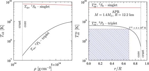
Left-hand panel: nucleon critical temperatures T_ck (k = n, p) versus density ρ for model 1. Right-hand panel: redshifted critical temperatures T^∞_ck versus radial coordinate r (in units of R) for model 1.

Open in new tab Download slide

Figure 2.

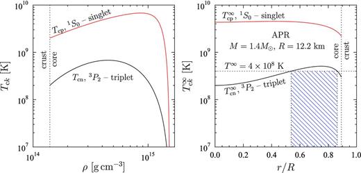
The same as in Fig. 1 but for model 2.

Open in new tab Download slide

The entrainment matrix Y_ik is calculated for the superfluidity models 1 and 2 in a way similar to how it was done in Kantor & Gusakov (2011).

When analysing viscous dissipation in oscillating NSs we allow for the damping due to shear and bulk viscosities. For the shear viscosity coefficient η we take the electron shear viscosity η_e, calculated in Shternin & Yakovlev (2008). We neglect the nucleon shear viscosity because (i) it is poorly known even for non-superfluid matter and (ii) it appears to be less than the electron shear viscosity in the core at T ≪ T_cp (Shternin & Yakovlev 2008).

The bulk viscosity coefficients are calculated as described by Gusakov (2007), Gusakov & Kantor (2008) and Kantor & Gusakov (2011). Since the direct URCA process is closed for our stellar model with M = 1.4 M_⊙, the main contributor to the bulk viscosity is the modified URCA process.

7.2 Oscillations of a non-superfluid star

As follows from Section 6.2, before considering oscillations of a superfluid NS one should study those of a normal (non-superfluid) star of the same mass. To this aim, we have determined the eigenfrequencies and eigenfunctions of the radial and non-radial oscillation modes for a non-superfluid NS of mass M = 1.4 M_⊙ and equation of state APR (see Section 7.1). We have solved the equations describing radial and non-radial perturbations of a non-rotating star in general relativity. These equations are derived by expanding the perturbed Einstein's equations in tensorial spherical harmonics in an appropriate gauge, and are integrated in the frequency domain.

Stellar modes are defined as solutions of the perturbed equations which are regular at the centre and with vanishing Lagrangian pressure perturbation at the surface, and (if l > 1) which behave as a pure outgoing wave at infinity; as discussed above, such solutions have complex frequencies ω = σ + i/τ. If l ≤ 1, instead, the frequency is real and the mode is not associated with gravitational emission.

The oscillation modes are classified according to the source of the restoring force which prevails in bringing the perturbed element of fluid back to the equilibrium position; for instance, we have a g mode if the restoring force is mainly provided by buoyancy, a p mode if it is due to a gradient of pressure and so on.

The radial modes are calculated as described in Gusakov et al. (2005). To calculate the non-radial modes we follow the formulation of Lindblom & Detweiler (1983) and Detweiler & Lindblom (1985). In their formulation, the equations for non-radial perturbations can be expressed, inside the star, as a system of first-order differential equations in the variables H₀, H₁, H₂, K, W_b and V_b defined in Section 5. Outside the star, they reduce to a simple, second-order differential equation (the Zerilli equation). By numerical integration of these equations (the procedure we have followed is described in detail e.g. in Burgio et al. 2011) we find, for each value of the multipolarity l, the (complex) eigenfrequencies ω and the corresponding eigenfunctions H₀(r), H₁(r), H₂(r), K(r), W_b(r) and V_b(r). The results of our computations are summarized in Table 1 and illustrated in Figs 3 and 4.

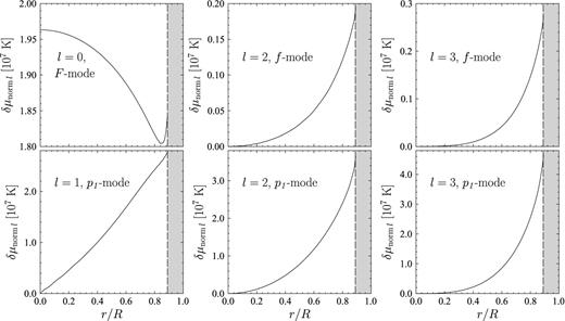
The function δμnorm l (in units of 107 K) versus r for fundamental radial F mode as well as for p1 and f modes with multipolarities l = 1, 2 and 3 (see the footnote 13). The energy of each oscillation mode is 1043 erg. Shaded region corresponds to crust, where δμnorm l is not defined and was not plotted.

Figure 3.

The function δμ_norm l (in units of 10⁷ K) versus r for fundamental radial F mode as well as for p₁ and f modes with multipolarities l = 1, 2 and 3 (see the footnote 13). The energy of each oscillation mode is 10⁴³ erg. Shaded region corresponds to crust, where δμ_norm l is not defined and was not plotted.

Open in new tab Download slide

Figure 4.

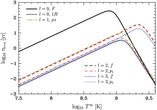
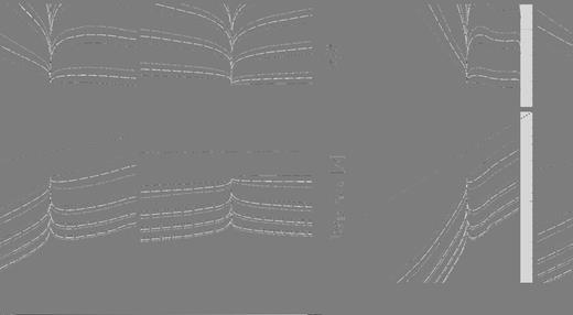
Damping times τ_{b + s} ≡ (τ^{− 1}_bulk + τ^{− 1}_shear)^{− 1} versus T^∞ for various oscillation modes. The effects of superfluidity are partially taken into account, as described in the text. Thick and thin solid lines correspond to radial (l = 0) F and 1H modes, respectively; dot–dashed line corresponds to dipole (l = 1) p₁ mode; thick and thin dashes correspond to quadrupole (l = 2) f and p₁ modes, respectively; and thick and thin dots correspond to octupole (l = 3) f and p₁ modes, respectively.

Open in new tab Download slide

Table 1.

Open in new tab

Frequency σ (in units of 10⁴ s⁻¹ and in units of |$\tilde{\sigma }=c/R \approx 2.46 \times 10^4$| s⁻¹) and the damping time τ_grav (in seconds) for various oscillation modes of a non-superfluid NS. The first column shows the multipolarity l of modes and their names.

l, mode	σ/(10⁴ s⁻¹)	\|$\sigma /\tilde{\sigma }$\|	τ_grav (s)
0, F	1.703	0.691	∞
0, 1H	4.080	1.656	∞
0, 2H	5.732	2.327	∞
1, p₁	2.893	1.175	∞
2, f	1.155	0.469	0.212
2, p₁	3.720	1.510	3.799
3, f	1.554	0.631	18.24
3, p₁	4.360	1.770	33.26

l, mode	σ/(10⁴ s⁻¹)	\|$\sigma /\tilde{\sigma }$\|	τ_grav (s)
0, F	1.703	0.691	∞
0, 1H	4.080	1.656	∞
0, 2H	5.732	2.327	∞
1, p₁	2.893	1.175	∞
2, f	1.155	0.469	0.212
2, p₁	3.720	1.510	3.799
3, f	1.554	0.631	18.24
3, p₁	4.360	1.770	33.26

Table 1.

Open in new tab

Frequency σ (in units of 10⁴ s⁻¹ and in units of |$\tilde{\sigma }=c/R \approx 2.46 \times 10^4$| s⁻¹) and the damping time τ_grav (in seconds) for various oscillation modes of a non-superfluid NS. The first column shows the multipolarity l of modes and their names.

l, mode	σ/(10⁴ s⁻¹)	\|$\sigma /\tilde{\sigma }$\|	τ_grav (s)
0, F	1.703	0.691	∞
0, 1H	4.080	1.656	∞
0, 2H	5.732	2.327	∞
1, p₁	2.893	1.175	∞
2, f	1.155	0.469	0.212
2, p₁	3.720	1.510	3.799
3, f	1.554	0.631	18.24
3, p₁	4.360	1.770	33.26

l, mode	σ/(10⁴ s⁻¹)	\|$\sigma /\tilde{\sigma }$\|	τ_grav (s)
0, F	1.703	0.691	∞
0, 1H	4.080	1.656	∞
0, 2H	5.732	2.327	∞
1, p₁	2.893	1.175	∞
2, f	1.155	0.469	0.212
2, p₁	3.720	1.510	3.799
3, f	1.554	0.631	18.24
3, p₁	4.360	1.770	33.26

Table 1 presents the real parts of the eigenfrequencies Re(ω) = σ (measured in units of 10⁴ s⁻¹ and in units of |$\tilde{\sigma } \equiv c/R \approx 2.46\times 10^4$| s⁻¹) and the characteristic gravitational damping times τ_grav (in seconds) for the modes with l = 0 (fundamental F mode and first two overtones 1H and 2H), l = 1 (dipole p₁ mode), l = 2 (quadrupole f and p₁ modes) and l = 3 (octupole f and p₁ modes).¹³ One can see that σ ≫ 1/τ_grav in all these cases. That is, damping due to emission of gravitational waves occurs on a time-scale much longer than the oscillation period.

Using definition (99) and equation (101) we have determined, in terms of the eigenfunctions H₀(r), H₁(r),…,V_b(r), the function δμ_norm l(r) and, consequently, the quantity δμ^∞_norm(r, θ) = δμ_norm l(r) Y⁰_l(θ) for each mode. As follows from equations (92) and (100), for a non-superfluid star δμ^∞_norm(r, θ) is simply a redshifted imbalance of chemical potentials, δμ^∞ = δμ^∞_norm. The function δμ_norm l(r), entering equation (98), is shown in Fig. 3 for the oscillation modes from Table 1. It is normalized such that the mechanical energy of oscillations is 10⁴³ erg. The shaded region corresponds to the crust of the star, where δμ_norm l(r) is not defined (protons are bound in nuclei there). As seen in the figure, |δμ_norm l(r)| for f modes is about one order of magnitude smaller than for p modes. This is not surprising, since matter is only weakly compressed during f mode oscillations, so that a deviation from beta-equilibrium (when δμ^∞ = 0) is small. The functions δμ_norm l(r) are employed to calculate the damping times of a superfluid NS in Section 7.4.

Fig. 4 shows the viscous damping time τ_{b + s} ≡ (τ^{− 1}_bulk + τ^{− 1}_shear)^{− 1} as a function of T^∞ for a set of oscillation modes. The solid lines correspond to radial (l = 0) modes F and 1H, dot–dashed line corresponds to dipole (l = 1) mode p₁, dashed lines correspond to quadrupole (l = 2) modes f and p₁, and dotted lines correspond to octupole (l = 3) modes f and p₁. To calculate τ_b+s we used the formulas for τ_bulk and τ_shear, applicable for the ordinary hydrodynamics of a non-superfluid liquid.¹⁴ However, we allow for the effects of superfluidity when calculating the kinetic coefficients η and ξ₂ (the other bulk viscous coefficients do not appear in the normal-fluid hydrodynamics). To calculate η and ξ₂ we adopt the nucleon superfluidity model 2 (see Section 7.1). Such an approximate approach to accounting for the effects of superfluidity is commonly used in the literature, but it is not fully consistent. The results of a more consistent approach (see Section 6) are discussed in Section 7.4.

As follows from Fig. 4, the dependence of τ_b+s on T^∞ is a power law at T^∞ ≲ 6 × 10⁸ K. At such T^∞ the proton superfluidity is ‘strong’ (T^∞ ≪ T^∞_cp). In that case the bulk viscosity is exponentially suppressed (Haensel, Levenfish & Yakovlev 2001), while the shear viscosity η ∝ 1/(T^∞)² (Shternin & Yakovlev 2008) and dominates. As a result, τ_b+s ∝ (T^∞)². At high enough temperatures T^∞ ≳ 6 × 10⁸ K the damping due to the bulk viscosity starts to prevail; this results in decreasing of τ_b+s with growing T^∞ (the curves in Fig. 4 bend down). At such T^∞ the neutrons are normal and the proton superfluidity is weak or absent. Neglecting the proton superfluidity, one obtains ξ₂ ∝ (T^∞)⁶ (Haensel et al. 2001), hence τ_b+s ∝ 1/(T^∞)⁶.

Let us note that the curves for f modes in Fig. 4 (thick dashed line and thick dots) bend down later than others; for them the shear viscosity is the dominant mechanism of damping up to T^∞ ≈ 2.0 × 10⁹ K. This is not surprising, since, as it was noted above, for f modes the deviation from beta-equilibrium is small (δμ^∞ is reduced by an order of magnitude in comparison to p modes, see Fig. 3); hence damping due to the bulk viscosity is suppressed (the relation between δμ^∞ and τ_bulk was discussed in detail e.g. in Gusakov et al. 2005). As a result, τ_b+s approaches its ‘bulk viscosity’ asymptote τ_b+s ∝ 1/T⁶ at higher temperatures T^∞ > 2.0 × 10⁹ K.

7.3 Frequency spectrum for superfluid NSs

First of all let us consider the frequency spectrum for radial oscillations of a superfluid NS employing the simplified model 1 of nucleon superfluidity. For such model this problem was discussed in detail by Kantor & Gusakov (2011), where it was solved exactly. Here we compare this exact solution with the approximate calculations obtained in the s = 0 approximation (see Section 6). Such a comparison is very useful, since it allows one to make a conclusion about applicability of the approximate approach in the case of non-radial oscillations, where the exact solution is not attempted.

The eigenfrequencies σ of radial pulsations (in units of |$\tilde{\sigma }$|⁠) versus T^∞₈ = T^∞/(10⁸ K) are shown in Figs 5(a)–(c). In Fig. 5(a) this dependence was obtained assuming that superfluid and normal modes are completely decoupled (s = 0 approximation). The thick solid lines demonstrate the first three normal (non-superfluid) radial modes F, 1H and 2H. As one expects, their frequencies do not depend on T^∞. The dashes are for the first six superfluid modes 1, …, 6, which are the solutions to equation (104). These modes, on the contrary, strongly depend on T^∞ and approach their temperature-independent asymptotes only at T^∞ ≲ 5 × 10⁷ K (when the entire NS core is superfluid and Y_ik does not depend on T^∞). At T^∞ > T^∞_cn max = 6 × 10⁸ K all neutrons are normal so that superfluid modes do not exist.

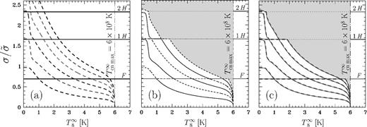
$Eigenfrequencies σ (in units of $\tilde{\sigma }$) of radial oscillations versus T∞8 = T∞/(108 K) for model 1 of nucleon superfluidity. (a) Approximate spectrum. First three normal modes (F, 1H and 2H) are shown by the solid lines; first six superfluid modes 1, …, 6 are shown by dashes. (b) Exact spectrum. Alternate solid and dashed lines show the first six exact modes (I, …, VI) of a radially oscillating star. No spectrum was plotted in the shaded region. (c) Approximate (dashed lines) and exact (solid lines) spectra. At T∞ > T∞cn max = 6 × 108 K all neutrons are normal and the spectrum is that of a non-superfluid star.$

Figure 5.

Eigenfrequencies σ (in units of |$\tilde{\sigma }$|⁠) of radial oscillations versus T^∞₈ = T^∞/(10⁸ K) for model 1 of nucleon superfluidity. (a) Approximate spectrum. First three normal modes (F, 1H and 2H) are shown by the solid lines; first six superfluid modes 1, …, 6 are shown by dashes. (b) Exact spectrum. Alternate solid and dashed lines show the first six exact modes (I, …, VI) of a radially oscillating star. No spectrum was plotted in the shaded region. (c) Approximate (dashed lines) and exact (solid lines) spectra. At T^∞ > T^∞_cn max = 6 × 10⁸ K all neutrons are normal and the spectrum is that of a non-superfluid star.

Open in new tab Download slide

Fig. 5(b) demonstrates the results of the exact solution to equations (83)–(101) obtained by Kantor & Gusakov (2011) for radial oscillations of a superfluid NS. The frequencies σ of the first six oscillation modes (I,…,VI) as functions of T^∞₈ are shown by alternate solid and dashed lines. No spectrum is plotted in the grey-shaded area. One can observe that the approximate spectrum (Fig. 5 a) is very similar to the exact spectrum (Fig. 5 b). However, there is one important difference: instead of crossings of superfluid and normal modes in Fig. 5(a) we have avoided crossings of the modes in Fig. 5(b). At these points the superfluid mode turns into the normal one and vice versa. As it was discussed in details in Gusakov & Kantor (2011) and Kantor & Gusakov (2011), this is not surprising, since in a vicinity of avoided crossings the Einstein equations (87) and superfluid equation (98) interact resonantly, so that approximation of completely decoupled superfluid and normal modes (s = 0) is inapplicable.¹⁵

For comparison, in Fig. 5(c) we plot both the approximate (dashed lines) and exact (solid lines) spectra. The agreement between both spectra is very good: the difference is less than a few per cent.

Such a close agreement of the exact and approximate results for radial oscillations allows us to analyse the spectrum of non-radial oscillations using the same approximation s = 0. The results of this analysis are shown in Fig. 6 for more realistic model 2 of nucleon superfluidity (see Section 7.1 and Fig. 2). Superfluid modes shown in this figure have been already studied in detail in our recent paper (Chugunov & Gusakov 2011). Thus, here we discuss them only briefly.

Figure 6.

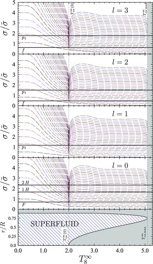
Eigenfrequencies σ versus T^∞ for model 2 of nucleon superfluidity and for multipolarities l = 0, 1, 2 and 3. For each l we plot first few normal modes (solid lines) and first 25 superfluid modes (dashed lines), whose eigenfunctions δμ_l differ by the number of radial nodes n. At T^∞ ≤ T^∞_cn(0) ≈ 2 × 10⁸ K (see the left vertical dotted line), neutron superfluidity occupies the stellar centre. The bottom panel demonstrates the variation of the SFL-region (shown by hatching) with T^∞. Shaded area in all panels shows the region where all neutrons are normal.

Open in new tab Download slide

Fig. 6 contains five panels. Four upper panels present eigenfrequencies σ as functions of T^∞₈ for normal modes from Table 1 (thick horizontal lines) and for superfluid modes (dashes) with multipolarities l = 0, 1, 2 and 3. For each l there is an infinite set of superfluid modes whose eigenfunctions δμ_l differ by the number of radial nodes n; in the figure we plot the first 25 of them. The lower panel demonstrates broadening of the SFL-region with decreasing T^∞₈ (SFL-region is shown by hatches). For model 2 (which we employ here) the redshifted neutron critical temperature T^∞_cn(r) has a maximum at T^∞_cn max ≈ 5.1 × 10⁸ K (right vertical dotted line). The neutron superfluidity reaches the stellar centre at T^∞ = T^∞_cn(0) ≈ 2 × 10⁸ K (left vertical dotted line). At T^∞ > T^∞_cn max all neutrons are normal, hence only normal modes exist in the star. At T^∞ < T^∞_cn(0) the core is completely occupied by the neutron superfluidity. One can see that the behaviour of superfluid modes differs strongly at T^∞ > T^∞_cn(0) and at T^∞ < T^∞_cn(0). This feature was discussed in Chugunov & Gusakov (2011) and Kantor & Gusakov (2011), where it was demonstrated that (roughly speaking) the frequencies σ of superfluid modes scale with Y_nn and R_sfl as |$\sigma \sim \sqrt{Y_{\rm nn}}/R_{\rm sfl}$|⁠, where R_sfl is the size of the SFL-region. With the increasing of temperature Y_nn decreases, while the size of the SFL-region can either decrease [at T^∞ > T^∞_cn(0)] or remain constant [at T^∞ < T^∞_cn(0)]. As a result, there is a partial compensation of these two tendencies at T^∞ > T^∞_cn(0) (hence, the frequency changes only weakly), while at T^∞ < T^∞_cn(0) the effect of decreasing of Y_nn is not compensated (hence, σ decreases with growing T^∞). At T^∞ ≲ 5 × 10⁷ K Y_ik does not depend on T^∞, and, as in the case of radial pulsations, the frequencies approach their low-temperature asymptotes.

7.4 Damping times for superfluid NSs

As in the case of eigenfrequencies, we first consider the e-folding times τ^{− 1}_{b + s} ≡ τ_bulk^{− 1} + τ^{− 1}_shear for radial (l = 0) pulsations for the simplified model 1 of nucleon superfluidity (see Fig. 1).

In Figs 7(a) and (d) we present the functions σ(T^∞) and τ_b+s(T^∞), obtained using the approximate method of Section 6.2. The frequencies and damping times are plotted for normal F mode (thick solid line) as well as for the first four superfluid modes 1, …, 4 (dashed lines).¹⁶ In the region shaded in grey the function τ_b+s(T^∞) for the normal mode was not plotted (there are too many merging resonances in this region). The dotted curve in Figs 7(d)–(f) labelled F_nfh (‘nfh’ is the abbreviation for ‘normal-fluid hydrodynamics’) shows the damping time calculated using the ordinary hydrodynamics of non-superfluid liquid but taking into account the effects of superfluidity on the bulk and shear viscosities. This curve is analogous to the thick solid curve in Fig. 4, obtained under the same conditions but for the model 2 of nucleon superfluidity. The vertical dotted line in Figs 7(a) and (d) indicates a temperature at which frequencies of normal F mode and the first superfluid mode coincide.

Figure 7.

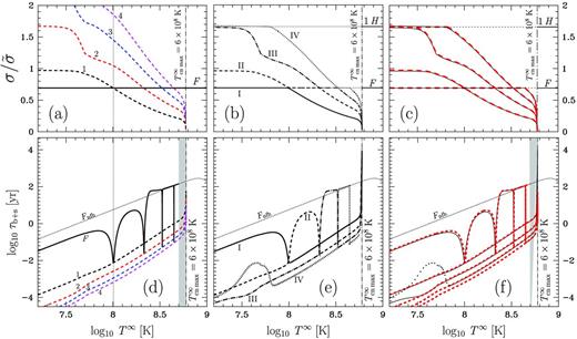
Eigenfrequencies σ (panels a–c) and damping times τ_b+s (panels d–f) of a radially oscillating NS versus T^∞ for model 1 of nucleon superfluidity. Panels (a) and (d): approximate solution (normal F mode and first four superfluid modes 1, …, 4 are shown by solid and dashed lines, respectively); panels (b) and (e): exact solution (first four exact modes I, …, IV are shown by solid, dashed, dot–dashed and dotted lines, respectively); panels (c) and (f): both approximate (dashed lines) and exact (solid lines) solutions. Panels (a)–(c) are the same spectra as those plotted, respectively, in Figs 5(a)–(c). Normal F mode is not shown in the shaded region because of technical reasons (too many resonances). Dotted lines in panels (d)–(f) show damping times for F mode calculated using ordinary normal-fluid hydrodynamics (see the text for more details). Part of the mode IV (at T^∞ < 6 × 10⁷ K) is shown by dots in the panel (f), as described in the text.

Open in new tab Download slide

We present a detailed analysis of Fig. 7(d) in what follows, together with description of the approximate solutions for non-radial oscillation modes (Figs 8 and 9).

Figure 8.

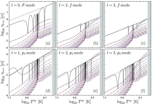
Damping times τ_b+s versus T^∞ for various oscillation modes for model 2 of nucleon superfluidity. On each panel we plot one normal mode (shown by solid line; its multipolarity and name is indicated) and first 15 superfluid modes (dashed lines). Dotted lines show τ_b+s(T^∞) for normal modes calculated using normal-fluid hydrodynamics (see the text for more details). In the shaded area all neutrons are normal and superfluid modes do not exist.

Open in new tab Download slide

Figure 9.

Eigenfrequencies σ (upper panels) and damping times τ_b+s (lower panels) versus T^∞ for quadrupole (l = 2) oscillation modes in an increasingly larger scale. The normal p₁ mode is shown by solid lines. Lower left-hand panel coincides with Fig. 8(e). Other lower panels are zoomed in versions of Fig. 8(e). Notations are the same as in Figs 6 and 8.

Open in new tab Download slide

For comparison, Figs 7(b) and (e) demonstrate the results of the exact calculation of frequencies σ(T^∞) and damping times τ_b+s(T^∞) for the first four (I,…,IV) oscillation modes of the superfluid NS [the modes are shown by solid (I), dashed (II), dot–dashed (III) and dotted (IV) lines].

To see how well the approximate solution (Figs 7 a and d) agrees with the exact one (Figs 7 b and e), both solutions are presented in Figs 7(c) and (f). Dashes correspond to approximate solution, and solid lines correspond to exact solution. A portion of the mode IV in Fig. 7(f) is shown by thick dots because the corresponding approximate solution (the mode 1H) is not plotted. One sees that the agreement between the approximate and exact solutions is reasonable everywhere (average error does not exceed 10–25 per cent) except for the resonances (see below) and an interval of temperatures T^∞ ≲ 3 × 10⁷ K where the mode III of exact solution deviates from the second superfluid mode of approximate solution. To explain this deviation let us note that, as follows from Fig. 5(a), at such T^∞ the frequency of the normal mode 1H practically coincides with that of the second superfluid mode. In that case equations (87) and (98) interact resonantly, so that the approximation of independent superfluid and normal modes is poor even though parameter s is small.¹⁷

Let us now consider the non-radial oscillations. Fig. 8 presents an approximate solution for the function τ_b+s(T^∞), which is obtained for a realistic nucleon superfluidity model 2. By dashes we show superfluid modes, and solid lines correspond to normal modes. Each panel in the figure is plotted for one normal mode (its name and multipolarity l are indicated) and for the first 15 superfluid modes with the same l. By dots, as in Figs 7(d)–(f), we plot τ_b+s for a corresponding normal modes calculated using the ordinary normal-fluid hydrodynamics. In the shaded region superfluid modes were not plotted because all neutrons are normal there and the star oscillates as a non-superfluid.

In more detail damping times are demonstrated for quadrupole (l = 2) oscillation modes in Fig. 9. In particular, the normal p₁ mode is shown there by solid lines. In the three lower panels we plot the dependence τ_b+s(T^∞) in an increasingly larger scale. In the three upper panels we plot, in the same scale, the oscillation frequencies σ(T^∞) (the corresponding spectrum was already presented in Fig. 6 in linear scale). Lower left-hand panel of Fig. 9 coincides with Fig. 8(e).

Let us discuss the main conclusions that can be drawn from the analysis of Figs 7(d), 8 and 9.

For any normal mode the dependence τ_b+s(T^∞) (solid lines in these figures) has a set of resonance features (spikes) concentrated (for radial and p modes) to the critical temperature T^∞_cn(0) at which neutron superfluidity in the core centre dies out. For model 1 T^∞_cn(0) = T_cn max^∞ = 6 × 10⁸ K (see Fig. 1), and for model 2 T^∞_cn(0) ≈ 2 × 10⁸ K (see Fig. 2). The resonances appear when frequency of the normal mode approaches the frequency of one of the superfluid modes. For instance, solid line in Fig. 7(a) crosses superfluid modes four times (in Figs 7 a and d, the temperature T^∞ of the first crossing is shown by the vertical dotted line and equals T^∞ ≈ 10⁸ K). Correspondingly, four resonances appear in Fig. 7(d). A similar situation can be observed in Figs 8 and 9. Near resonances τ_b+s for normal mode rapidly decreases by one to two orders of magnitude (see item 2) and, in the resonance point, it becomes strictly equal to τ_b+s for the corresponding superfluid mode.
Such behaviour of the approximate solution τ_b+s(T^∞) for normal modes in the vicinity of resonances can be easily understood. In resonance points, in which the frequencies of superfluid and normal modes coincide, equation (98) has a non-trivial solution even in the absence of the source δμ_norm l. For it to be satisfied with the source, the oscillation amplitude δμ must be infinitely large. In other words, in resonance points all the energy must be contained in superfluid degrees of freedom (in particular, near resonances W_sfl ≫ W_b and V_sfl ≫ V_b). Formally, this means that in the resonance point the damping time τ_b+s should be exactly the same as for the superfluid mode.
Another important point that is worth noting is that, as follows from Fig. 7(f), the approximate solution for the normal radial F mode describes qualitatively well the exact solution near resonances (the latter is shown by solid lines). We expect that the same is also true for non-radial modes for which the exact solution was not attempted. At first glance such an agreement between the approximate and exact solutions seems surprising because the approximation s = 0 should not work in the vicinity of resonances, where the frequencies of superfluid and normal modes are close to each other. Nevertheless, one verifies that this approximation is still suitable for a qualitatively correct description of the function τ_b+s(T^∞) if one bears in mind that (i) close to any resonance the exact solution is a linear superposition of independent solutions describing (intersecting) superfluid and normal modes and (ii) τ_b+s for the superfluid mode is much less than for the normal mode.
Items (i) and (ii) mean that, in the exact solution, the main contribution to τ_b+s comes from the superfluid mode (while the contribution from the normal mode is small). This leads us to conclusion that the superfluid modes are the main sources of viscous dissipation in the vicinity of resonance points. The same conclusion was already drawn above using the approximate method of Section 6.2. This explains why the approximate method gives qualitatively correct results for τ_b+s(T^∞) near resonances.
In order to avoid confusion let us emphasize that the function τ_b+s(T^∞) contains resonance features (spikes) for normal modes only in the approximate solution (see Figs 7 d, 8 and 9). In the exact solution any normal oscillation mode turns into a superfluid one near resonance (and vice versa). This leads to an abrupt decreasing (increasing) of τ_b+s and formation of a ‘step-like’ structure rather than spike (see Fig. 7 e).
It was already mentioned above that, as follows from Figs 7(d), 8 and 9, normal modes (far from resonances) damp out by one to two orders of magnitude slower than those superfluid modes with which they can have equal frequencies (i.e. intersect in the σ-T^∞ plane).
What is the reason for such a fast damping of superfluid modes? To be more concrete, below we consider a low-temperature case, T^∞ ≲ 3 × 10⁷ K. There are three main factors: (i) for superfluid modes eigenfunctions W_sfl and V_sfl have a maximum in the central regions of a star where the shear viscosity is maximal. On the contrary, for normal modes the maximum of eigenfunctions W_b and V_b lies closer to the NS surface, where the shear viscosity coefficient can be substantially (five and more times) smaller. As a consequence, |$\mathfrak {W}_{\rm shear}$| for superfluid modes turns out to be greater (and hence τ_shear smaller) than for normal modes. (ii) The energy of superfluid modes is given by equation (73) and depends on the quantity y (see equation 68 for the definition of y). At low T^∞ the parameter y is small, y ∼ n_p/n_n ∼ 0.04-0.09, which also results in decreasing of the characteristic damping times for superfluid modes.¹⁸ (iii) This factor is particularly important for radial oscillations (l = 0) and is related to a coefficient α₁ in expression (78) for the damping time τ_shear due to shear viscosity. This coefficient is given by equation (81) which is a sum of four terms. It turns out that for the normal radial modes the first term is well compensated by the third term H₂, while the other terms vanish. For the superfluid modes such compensation does not occur because for them H₂ = 0.
At low enough T^∞ the damping times for normal radial and p modes can be several times larger or smaller than τ_b+s, calculated employing ordinary hydrodynamics of non-superfluid liquid but accounting for the effects of superfluidity on the bulk and shear viscosity coefficients (dotted lines in Figs 7 d, 8 a, d, e and f, and 9). Let us inspect, for example, Fig. 8(a). One sees that at T^∞ ≲ 10⁸ K, τ_b+s, calculated in the frame of non-superfluid hydrodynamics, is approximately four times larger than τ_b+s determined self-consistently. This difference arises because to plot the dotted curve we used the formulas of Section 4 in which W_sfl = V_sfl = 0. As T^∞ grows, however, the difference in two ways of calculating τ_b+s rapidly decreases because the SFL-region becomes smaller and hence its contribution to τ_b+s becomes less and less pronounced.
Unlike the radial and p modes, the agreement between dotted and solid lines for normal f modes is very good (see Figs 8 b and c), which means that for these modes use of the non-superfluid hydrodynamics (far from resonances) is well justified. The reason for such a good agreement of damping times is related to a relatively weak compression–decompression of matter in the course of the f-type oscillations. As a consequence, for the normal f modes the source δμ_norm l in equation (98) is small, so that far from the resonances δμ ≈ 0 and the superfluid degrees of freedom are almost not excited (W_sfl ≈ V_sfl ≈ 0, see equations 48, 52 and 90). This result confirms, extends and, we think, provides a deeper understanding of the results previously obtained in a Newtonian framework by e.g. Lindblom & Mendell (1994) and Andersson et al. (2009).
At T^∞ → T^∞_cn max = 6 × 10⁸ K, one can observe the rapid increasing of τ_b+s for superfluid modes in Fig. 7. It is bounded from above by τ_bulk and is related with the tendency of τ_shear to grow to infinity in this limit. Such a behaviour of τ_shear was discussed in detail in Kantor & Gusakov (2011) and is specific for model 1 of nucleon superfluidity.

8 SUMMARY

In this paper we, for the first time, self-consistently analyse the effects of nucleon superfluidity on damping of oscillations of non-rotating general relativistic NSs. Our main results are summarized below.

The analytic formulas are derived for the oscillation energy E_mech (71) and for the characteristic damping times τ_bulk (77) and τ_shear (78) due to the bulk and shear viscosities. These expressions are valid for oscillations of arbitrary multipolarity l. Expression (71) for E_mech is the generalization of formula (26) of Thorne & Campolattaro (1967), written for a non-superfluid NS. Expressions (77) and (78) are the generalizations, to the case of superfluidity, of formulas (5) and (6) in Cutler et al. (1990). Note that the damping times, calculated using the formulas of Cutler et al. (1990), appear to be two times smaller than our τ_bulk and τ_shear, calculated from equations (77) and (78) under assumption that superfluid degrees of freedom are suppressed (i.e. W_sfl = V_sfl = 0).
An approximate method is developed in detail and applied, which allows one to easily determine the eigenfrequencies and eigenfunctions of an oscillating superfluid NS, provided that they are known for a normal (non-superfluid) star of the same mass (see Section 6.2). The method is based on the approximate decoupling of equations describing superfluid and normal oscillation modes and exploits the ideas first formulated in Gusakov & Kantor (2011) and Chugunov & Gusakov (2011).
Using radial oscillations as an example, and adopting the simplified model 1 of nucleon superfluidity (Fig. 1), we demonstrate that this method leads to oscillation frequencies and characteristic damping times that agree well with the results of exact calculation.
The approximate method of Section 6.2 is applied to study non-radial oscillations of a superfluid NS assuming the realistic model 2 of nucleon superfluidity (Fig. 2). A number of normal and superfluid oscillation modes with multipolarities l = 0, …, 3 are considered. In particular, the following normal modes are analysed: F mode for l = 0, p₁ mode for l = 1 and f and p₁ modes for l = 2 and 3.

We demonstrate the following.

As a rule, for any given normal mode (whose frequency σ coincides with the corresponding frequency of a non-superfluid NS and does not depend on the internal redshifted stellar temperature T^∞), the viscous damping time τ_{b + s} ≡ (τ^{− 1}_bulk + τ^{− 1}_shear)^{− 1} is one order of magnitude greater than τ_b+s for those superfluid modes that can intersect the normal mode in the σ-T^∞ plane. This effect is non-local (occurs only after integration over the NS volume) and is determined by a number of factors (see item 2 of Section 7.4).
The function τ_b+s(T^∞) for any normal mode contains resonance features. In resonance points the frequency σ of a normal mode coincides with that of some of the superfluid modes (their σ depends on T^∞). When passing a resonance (e.g. with growing T^∞), τ_b+s initially rapidly decreases (by one to two orders of magnitude) until it reaches the value of τ_b+s for this superfluid mode and, after that, it increases again (see Figs 7 d, 8 and 9).
Resonance features (spikes) appear only in the approximate treatment of Section 6, in which the normal and superfluid modes intersect at resonance points (see e.g. Fig. 5 a). In the exact solution instead of crossings one has avoided crossings of modes (Fig. 5 b). Near avoided crossings any real mode changes its behaviour from normal-like to superfluid-like (and vice versa). As a result, instead of spikes one has a very rapid step-like decreasing (increasing) of τ_b+s (cf. Figs 7d and e).
Sufficiently far from the resonances τ_b+s for normal radial and p modes, determined self-consistently employing the hydrodynamics of a superfluid liquid, can differ several fold from τ_b+s, calculated using the ordinary normal-fluid hydrodynamics (but accounting for the effects of superfluidity on the shear and bulk viscosities). The latter approximation is often adopted in the literature devoted to oscillations of NSs.
In contrast to radial and p modes, for f modes far from the resonances, use of the ordinary hydrodynamics of non-superfluid liquid for calculation of τ_b+s is well justified. The reason is that for f-type oscillations the imbalance δμ of chemical potentials is relatively small (matter does not compress significantly during oscillations). Thus, superfluid degrees of freedom are almost not excited (see Sections 6.2 and 7.4).
Since for f modes far from the resonances δμ is small (i.e. deviation from the beta-equilibrium is weak), bulk viscous damping of f modes is suppressed in comparison to p modes.

Though here we only considered oscillations of superfluid non-rotating NSs, we expect that the main conclusions of this work will also remain (mostly) unchanged for rotating NSs. Our results indicate that dissipative evolution of oscillating NSs may follow quite different scenarios than those usually considered in the literature. This is especially true if one is interested in the combined analysis of damping of oscillations and thermal evolution of an NS or in the analysis of instability windows, which are the values of T^∞ and rotation frequency at which a star becomes unstable with respect to the emission of gravitational waves (e.g. the r mode instability; see Andersson 1998; Friedman & Morsink 1998). These issues are extremely interesting and important, but we left them beyond the scope of this paper and will address the related topics in our subsequent publication.

This study was supported by the Dynasty Foundation, Ministry of Education and Science of Russian Federation (contract No. 11.G34.31.0001 with SPbSPU and leading scientist G. G. Pavlov, and agreement No. 8409, 2012), RFBR (11-02-00253-a, 12-02-31270-mol-a), FASI (grant NSh-4035.2012.2), RF president programme (grant MK-857.2012.2), by the RAS presidium programme ‘Support for young scientists’, and by CompStar, a Research Networking Programme of the European Science Foundation.

1

Note that, in Gusakov (2007), there is an additional term in the expression for S^μ, so that

\begin{eqnarray*} S^{\mu } = S u^{\mu } - {u_{\nu } \over T} \,\, \tau ^{\mu \nu } - {\varkappa _{\rm n} \over T} \,\, Y_{{\rm n}k} w^{\mu }_{(k)}. \end{eqnarray*}

The last term here appears naturally in the entropy generation equation. However, strictly speaking, it is small and should be neglected if one takes into account only the largest dissipative terms in the equations of superfluid hydrodynamics (this is the standard approximation; see Gusakov 2007 and section 140 of Landau & Lifshitz 1987 for an explanation of what we mean by the ‘largest terms’). It remains to note that the terms similar to the last term in the expression for S^μ also appear in the most general form of the non-relativistic superfluid dissipative hydrodynamics formulated by Clark (for details see the book by Putterman 1974).

2

This equality holds true only if one neglects the thermal conductivity, as we assume in equation (12).

3

A more detailed argument can be found in Thorne & Campolattaro (1967); see also Regge & Wheeler (1957).

4

However, beyond the linear approximation, equations (4), (5), (19) and (20) yield U_(b) μU^μ_(b) = −1 + Y_niY_nk w_(i) μw^μ_(k)/n²_b. The normalization condition (45) is generally not fulfilled because the reference frame in which U^μ_(b) = (1, 0, 0, 0) is not comoving [i.e. j^μ_(b)U_(b) μ ≠ −n_b in that reference frame]. As it was already indicated in Section 2, all thermodynamic variables are measured in the reference frame, in which u^μ = (1, 0, 0, 0).

5

This expression is analogous to the corresponding formula for the kinetic energy density of a non-relativistic superfluid mixture, obtained by Andreev & Bashkin (1975), see their equation (7).

6

It is worth to make a number of comments on equation (89): (i) in Gusakov & Kantor (2011) this equation was derived under the assumption that the only superfluid species are neutrons (i.e. Y_pi = 0). A generalization of this equation to the case of possible proton superfluidity is presented in (Chugunov & Gusakov 2011, see their equation 3). (ii) In both papers (Chugunov & Gusakov 2011; Gusakov & Kantor 2011), this equation is written with the same mistake. In particular, in Chugunov & Gusakov (2011) one should write n_e ∂_j(e^ν/2 δμ) instead of n_e e^ν/2 ∂_j(δμ) in the right-hand side of equation (3).

7

The equality ∂ε(n_b, n_e)/∂n_e = −δμ follows from the second law of thermodynamics (15), which can be rewritten in our case as dε = μ_n dn_b − δμ dn_e.

8

Here and below by ‘normal modes’ we mean oscillation modes (of approximate solution) that also exist in the normal (non-superfluid) star.

9

This is the main advantage of treating |$\tilde{s}$| in a non-perturbative way. Note, however, that this trick leads to somewhat ‘excessive’ accuracy of the approximate solution to oscillation equations: the retained terms depending on |$\tilde{s}$| may lead to smaller correction to the solution than the s-dependent terms which were ignored. Bearing this in mind and with the aim to simplify consideration, in Gusakov & Kantor (2011) it was assumed that both parameters s and |${\tilde{s}}$| vanish in the s = 0 approximation. Such an approach is also possible. In that case, strictly speaking, the resulting Einstein equations would differ slightly from the equations describing oscillations of a non-superfluid NSs. In particular, instead of the standard adiabatic index of the ‘frozen’ npe-matter γ_fr = (n_b/P)[∂P(n_b, x_e)/∂n_b], the new index would appear, γ = (n_b/P)[∂P(n_b, n_e)/∂n_b]. However, this difference is not essential, because s and |$\tilde{s}$| are small.

10

The corresponding equation (5) of Chugunov & Gusakov (2011) contains a mistake that was corrected in the second version of the manuscript in arXiv (see arXiv:1107.4242v2).

11

In this paper, in all numerical calculations we used σ instead of ω in equation (98), because σ ≫ 1/τ_grav. Also, when calculating δμ_norm l we only employed the real parts of eigenfunctions H₀, H₁, H₂, K, W_b and V_b (see a note after equation 73).

12

Fig. 2 is a slightly modified version of fig. 1 from Chugunov & Gusakov (2011).

13

The f mode is absent in the case of l = 1.

14

More precisely, we used equations (77) and (78) with W_sfl = V_sfl = 0.

15

Thus, it would not be correct to say that any real oscillation mode of a superfluid star is either purely superfluid or purely normal: for some T^∞ it can show itself as a superfluid, but for other T^∞ it can behave as a normal mode (see Fig. 5b).

16

Note that, in Figs 7(a)–(c) we present, in logarithmic scale, parts of the spectra, which were already plotted in linear scale in Figs 5(a)–(c), respectively.

17

For a quantitatively correct description of the function τ_b+s(T^∞) in that case it is, in principle, straightforward to develop a perturbation theory similar to the degenerate perturbation theory of quantum mechanics (see below the discussion of resonances in Figs 7–9).

18

To get an estimate for y we made use of the sum rule μ_nY_nn + μ_pY_np = n_n valid at T^∞ = 0 (Gusakov, Kantor & Haensel 2009a), and neglected the small matrix element Y_np in comparison with Y_nn.

REFERENCES

Abbott

B.

et al. ,

Phys. Rev. D

,

2007

, vol.

76

pg.

062003

Crossref

Search ADS

Akmal

A.

Pandharipande

V. R.

Ravenhall

D. G.

,

Phys. Rev. C

,

1998

, vol.

58

pg.

1804

Crossref

Search ADS

Andersson

N.

,

ApJ

,

1998

, vol.

502

pg.

708

Crossref

Search ADS

Andersson

N.

,

Classical Quantum Gravity

,

2003

, vol.

20

pg.

R105

Crossref

Search ADS

Andersson

N.

Kokkotas

K. D.

,

Int. J. Mod. Phys. D

,

2001

, vol.

10

pg.

381

Crossref

Search ADS

Andersson

N.

Comer

G. L.

Langlois

D.

,

Phys. Rev. D

,

2002

, vol.

66

pg.

104002

Crossref

Search ADS

Andersson

N.

Glampedakis

K.

Haskell

B.

,

Phys. Rev. D

,

2009

, vol.

79

pg.

103009

Crossref

Search ADS

Andersson

N.

Ferrari

V.

Jones

D. I.

Kokkotas

K. D.

Krishnan

B.

Read

J. S.

Rezzolla

L.

Zink

B.

,

Gen. Relativ. Gravitation

,

2011

, vol.

43

pg.

409

Crossref

Search ADS

Andreev

A. F.

Bashkin

E. P.

,

Zh. Eksp. Teor. Fiz.

,

1975

, vol.

69

pg.

319

Burgio

G. F.

Ferrari

V.

Gualtieri

L.

Schulze

H.-J.

,

Phys. Rev. D

,

2011

, vol.

84

pg.

044017

Crossref

Search ADS

Carter

B.

Khalatnikov

I. M.

,

Phys. Rev. D

,

1992

, vol.

45

pg.

4536

Crossref

Search ADS

Chamel

N.

Haensel

P.

,

Living. Rev. Relativ.

,

2008

, vol.

11

pg.

10

Crossref

Search ADS

Chandrasekhar

S.

,

ApJ

,

1964

, vol.

140

pg.

417

Crossref

Search ADS

Chandrasekhar

S.

Ferrari

V.

,

Proc. R. Soc. Lond. A

,

1991

, vol.

432

pg.

247

Crossref

Search ADS

Chugunov

A. I.

Gusakov

M. E.

,

MNRAS

,

2011

, vol.

418

pg.

L54

Crossref

Search ADS

Chugunov

A. I.

Yakovlev

D. G.

,

Astron. Rep.

,

2005

, vol.

49

pg.

724

Crossref

Search ADS

Comer

G. L.

Langlois

D.

Lin

L. M.

,

Phys. Rev. D

,

1999

, vol.

60

pg.

104025

Crossref

Search ADS

Cutler

C.

Lindblom

L.

,

ApJ

,

1987

, vol.

314

pg.

234

Crossref

Search ADS

Cutler

C.

Lindblom

L.

Splinter

R. J.

,

ApJ

,

1990

, vol.

363

pg.

603

Crossref

Search ADS

Detweiler

S. L.

Ipser

J. R.

,

ApJ

,

1973

, vol.

185

pg.

685

Crossref

Search ADS

Detweiler

S.

Lindblom

L.

,

ApJ

,

1985

, vol.

292

pg.

12

Crossref

Search ADS

Epstein

R. I.

,

ApJ

,

1988

, vol.

333

pg.

880

Crossref

Search ADS

Friedman

J. L.

Morsink

S. M.

,

ApJ

,

1998

, vol.

502

pg.

714

Crossref

Search ADS

Gusakov

M. E.

,

Phys. Rev. D

,

2007

, vol.

76

pg.

083001

Crossref

Search ADS

Gusakov

M. E.

Andersson

N.

,

MNRAS

,

2006

, vol.

372

pg.

1776

Crossref

Search ADS

Gusakov

M. E.

Kantor

E. M.

,

Phys. Rev. D

,

2008

, vol.

78

pg.

083006

Crossref

Search ADS

Gusakov

M. E.

Kantor

E. M.

,

Phys. Rev. D

,

2011

, vol.

83

pg.

081304

Crossref

Search ADS

Gusakov

M. E.

Kaminker

A. D.

Yakovlev

D. G.

Gnedin

O. Y.

,

A&A

,

2004

, vol.

423

pg.

1063

Crossref

Search ADS

Gusakov

M. E.

Yakovlev

D. G.

Gnedin

O. Y.

,

MNRAS

,

2005

, vol.

361

pg.

1415

Crossref

Search ADS

Gusakov

M. E.

Kantor

E. M.

Haensel

P.

,

Phys. Rev. C

,

2009a

, vol.

79

pg.

055806

Crossref

Search ADS

Gusakov

M. E.

Kantor

E. M.

Haensel

P.

,

Phys. Rev. C

,

2009b

, vol.

80

pg.

015803

Crossref

Search ADS

Haensel

P.

Levenfish

K. P.

Yakovlev

D. G.

,

A&A

,

2001

, vol.

372

pg.

130

Crossref

Search ADS

Haskell

B.

Andersson

N.

,

MNRAS

,

2010

, vol.

408

pg.

1897

Crossref

Search ADS

Haskell

B.

Andersson

N.

Passamonti

A.

,

MNRAS

,

2009

, vol.

397

pg.

1464

Crossref

Search ADS

Heinke

C. O.

Ho

W. C. G.

,

ApJ

,

2010

, vol.

719

pg.

L167

Crossref

Search ADS

Heiselberg

H.

Hjorth-Jensen

M.

,

ApJ

,

1999

, vol.

525

pg.

L45

Crossref

Search ADS

Ipser

J. R.

Thorne

K. S.

,

ApJ

,

1973

, vol.

181

pg.

181

Crossref

Search ADS

Israel

G. L.

et al. ,

ApJ

,

2005

, vol.

628

pg.

L53

Crossref

Search ADS

Kantor

E. M.

Gusakov

M. E.

,

Phys. Rev. D

,

2009

, vol.

79

pg.

043004

Crossref

Search ADS

Kantor

E. M.

Gusakov

M. E.

,

Phys. Rev. D

,

2011

, vol.

83

pg.

103008

Crossref

Search ADS

Khalatnikov

I. M.

,

An Introduction to the Theory of Superfluidity

,

1989

New York

Addison-Wesley

Google Scholar

Google Preview

OpenURL Placeholder Text

WorldCat

Khalatnikov

I. M.

Lebedev

V. V.

,

Phys. Lett. A

,

1982

, vol.

91

pg.

70

Crossref

Search ADS

Kokkotas

K. D.

Schmidt

B.

,

Living Rev. Relativ.

,

1999

, vol.

2

pg.

2

Crossref

Search ADS

Kokkotas

K. D.

Schutz

B. F.

,

MNRAS

,

1992

, vol.

255

pg.

119

Crossref

Search ADS

Landau

L. D.

Lifshitz

E. M.

,

Fluid Mechanics. Course of Theoretical physics

,

1987

Oxford

Pergamon Press

Google Scholar

Google Preview

OpenURL Placeholder Text

WorldCat

Lee

U.

,

A&A

,

1995

, vol.

303

pg.

515

Lee

U.

Yoshida

S.

,

ApJ

,

2003

, vol.

586

pg.

403

Crossref

Search ADS

Lindblom

L.

Detweiler

S. L.

,

ApJS

,

1983

, vol.

53

pg.

73

Crossref

Search ADS

Lindblom

L.

Mendell

G.

,

ApJ

,

1994

, vol.

421

pg.

689

Crossref

Search ADS

Lindblom

L.

Mendell

G.

,

ApJ

,

1995

, vol.

444

pg.

804

Crossref

Search ADS

Lindblom

L.

Mendell

G.

,

Phys. Rev. D

,

2000

, vol.

61

pg.

104003

Crossref

Search ADS

Lin

L.-M.

Andersson

N.

Comer

G. L.

,

Phys. Rev. D

,

2008

, vol.

78

pg.

083008

Crossref

Search ADS

Lombardo

U.

Schulze

H.-J.

Blaschke

D.

Glendenning

N. K.

Sedrakian

A.

,

Lecture Notes in Phys. Vol. 578. Physics of Neutron Star Interiors

,

2001

Berlin

Springer

pg.

30

Google Scholar

Google Preview

OpenURL Placeholder Text

WorldCat

Meltzer

D. W.

Thorne

K. S.

,

ApJ

,

1966

, vol.

145

pg.

514

Crossref

Search ADS

Mendell

G.

,

ApJ

,

1991a

, vol.

380

pg.

515

Crossref

Search ADS

Mendell

G.

,

ApJ

,

1991b

, vol.

380

pg.

530

Crossref

Search ADS

Negele

J. W.

Vautherin

D.

,

Nucl. Phys. A

,

1973

, vol.

207

pg.

298

Crossref

Search ADS

Owen

B.

,

Phys. Rev. D

,

2010

, vol.

82

pg.

104002

Crossref

Search ADS

Page

D.

Lattimer

J. M.

Prakash

M.

Steiner

A. W.

,

ApJS

,

2004

, vol.

155

pg.

623

Crossref

Search ADS

Page

D.

Prakash

M.

Lattimer

J. M.

Steiner

A. W.

,

Phys. Rev. Lett.

,

2011

, vol.

106

pg.

081101

Crossref

Search ADS

PubMed

Passamonti

A.

Andersson

N.

,

MNRAS

,

2011

, vol.

413

pg.

47

Crossref

Search ADS

Passamonti

A.

Andersson

N.

,

MNRAS

,

2012

, vol.

419

pg.

638

Crossref

Search ADS

Passamonti

A.

Glampedakis

K.

,

MNRAS

,

2012

, vol.

422

pg.

3327

Crossref

Search ADS

Prix

R.

Rieutord

M.

,

A&A

,

2002

, vol.

393

pg.

949

Crossref

Search ADS

Prix

R.

Comer

G. L.

Andersson

N.

,

MNRAS

,

2004

, vol.

348

pg.

625

Crossref

Search ADS

Putterman

S. J.

,

Superfluid Hydrodynamics

,

1974

Amsterdam

North-Holland

Regge

T.

Wheeler

J. A.

,

Phys. Rev.

,

1957

, vol.

108

pg.

1063

Crossref

Search ADS

Reisenegger

A.

,

ApJ

,

1995

, vol.

442

pg.

749

Crossref

Search ADS

Samuelsson

L.

Andersson

N.

,

Classical Quantum Gravity

,

2009

, vol.

26

pg.

155016

Crossref

Search ADS

Shternin

P. S.

Yakovlev

D. G.

,

Phys. Rev. D

,

2008

, vol.

78

pg.

063006

Crossref

Search ADS

Shternin

P. S.

Yakovlev

D. G.

Heinke

C. O.

Ho

W. C. G.

Patnaude

D. J.

,

MNRAS

,

2011

, vol.

412

pg.

L108

Crossref

Search ADS

Strohmayer

T. E.

Watts

A. L.

,

ApJ

,

2005

, vol.

632

pg.

111

Crossref

Search ADS

Strohmayer

T. E.

Watts

A. L.

,

ApJ

,

2006

, vol.

653

pg.

593

Crossref

Search ADS

Thorne

K. S.

Campolattaro

A.

,

ApJ

,

1967

, vol.

49

pg.

591

Crossref

Search ADS

Watts

A. L.

Bertulani

C. A.

Piekarewicz

J.

,

2011

to appear as a chapter in the book ‘Neutron Star Crust’, preprint (arXiv:1111.0514)

Watts

A. L.

Strohmayer

T. E.

,

Adv. Space Res.

,

2007

, vol.

40

pg.

1446

Crossref

Search ADS

Wong

K. S.

Lin

L. M.

Leung

P. T.

,

ApJ

,

2009

, vol.

699

pg.

1809

Crossref

Search ADS

Yakovlev

D. G.

Pethick

C. J.

,

ARA&A

,

2004

, vol.

42

pg.

169

Crossref

Search ADS

Yakovlev

D. G.

Levenfish

K. P.

Shibanov

Yu.A.

,

Phys. Usp.

,

1999

, vol.

42

pg.

737

Crossref

Search ADS

Yoshida

S.

Lee

U.

,

Phys. Rev. D

,

2003a

, vol.

67

pg.

124019

Crossref

Search ADS

Yoshida

S.

Lee

U.

,

MNRAS

,

2003b

, vol.

344

pg.

207

Crossref

Search ADS

APPENDIX A: BOUNDARY CONDITIONS TO EQUATION (98)

Equation (98) should be solved in the region of an NS core where neutrons are superfluid (SFL-region). If the NS centre is occupied by the neutron superfluidity, then for regularity of the solution at r → 0 it is necessary that

\begin{equation} \delta \mu _{l} \propto r^l. \end{equation}

(A1)

The conditions at the boundary of the SFL-region follow from the requirement of the absence of particle transfer (baryons and electrons) through the interface. One obtains from definitions (4)–(7)

\begin{equation} {\pmb X}_{\bot }=0, \end{equation}

(A2)

where |${\pmb X}_{\bot }$| is the component of the vector X^j perpendicular to the interface. To rewrite equation (A2) in terms of δμ_l(r), it is necessary to consider two possibilities.

The boundary (one of the boundaries) between the SFL-region and non-superfluid matter lies inside the core and is defined by the condition T = T_cn(R_b) (R_b is the radial coordinate of the boundary). Then at the boundary Y_nn(R_b) = Y_np(R_b) = 0 and from equations (90) and (98), one has
\begin{equation} \delta \mu _l^\prime =\frac{{\rm e^{\lambda -\nu /2} \, \omega ^2}}{h^\prime \, \mathfrak {B}}\, (\delta \mu _l - \delta \mu _{{\rm norm} \, l}). \end{equation}
(A3)
Outer boundary of the SFL-region coincides with the crust–core interface (R_b = R_cc). In that case T < T_cn(R_cc) [i.e. Y_nn(R_cc) and Y_np(R_cc) are non-zero] and from equation (90) it follows that
\begin{equation} \delta \mu _{l}^\prime (R_{\rm cc})=0. \end{equation}
(A4)
The conditions (A1)–(A4) are necessary and sufficient for solving equation (98).

Download all slides

Month:	Total Views:
February 2017	2
March 2017	1
June 2017	2
August 2017	3
September 2017	1
October 2017	4
November 2017	1
December 2017	6
January 2018	3
February 2018	2
March 2018	4
April 2018	11
May 2018	6
June 2018	3
July 2018	7
August 2018	7
September 2018	2
October 2018	8
November 2018	5
December 2018	7
January 2019	4
February 2019	5
March 2019	9
April 2019	7
May 2019	9
June 2019	5
July 2019	6
August 2019	5
September 2019	4
October 2019	7
November 2019	13
December 2019	5
January 2020	7
February 2020	5
March 2020	7
April 2020	4
May 2020	3
June 2020	6
July 2020	4
August 2020	4
September 2020	4
October 2020	9
November 2020	3
December 2020	3
January 2021	3
February 2021	6
March 2021	8
April 2021	3
May 2021	2
June 2021	8
July 2021	3
August 2021	5
September 2021	13
October 2021	6
November 2021	5
December 2021	5
January 2022	1
February 2022	7
March 2022	8
April 2022	13
May 2022	6
June 2022	2
July 2022	11
August 2022	15
September 2022	6
October 2022	13
November 2022	7
December 2022	5
January 2023	14
February 2023	2
March 2023	10
April 2023	13
June 2023	6
July 2023	9
August 2023	9
September 2023	4
October 2023	4
November 2023	3
December 2023	15
January 2024	7
February 2024	6
March 2024	6
April 2024	6
May 2024	7
June 2024	16
July 2024	9
August 2024	3
September 2024	15
October 2024	17
November 2024	9
December 2024	6
January 2025	2
February 2025	11
March 2025	8
April 2025	8

Article Contents

Dissipation in relativistic superfluid neutron stars

Abstract

1 INTRODUCTION

2 DISSIPATIVE SUPERFLUID HYDRODYNAMICS

3 BASIC EQUATIONS

3.1 An unperturbed star

3.2 Small departures from equilibrium

4 DAMPING OF OSCILLATIONS DUE TO THE BULK AND SHEAR VISCOSITIES: GENERAL FORMULAS

4.1 Mechanical energy

4.2 Dissipation rates

5 OSCILLATION EQUATIONS

6 OUR APPROACH

6.1 Decoupling of superfluid and normal modes

6.2 A strategy to calculate the damping times

7 RESULTS

7.1 Microphysics input and equilibrium model

7.2 Oscillations of a non-superfluid star

7.3 Frequency spectrum for superfluid NSs

7.4 Damping times for superfluid NSs

8 SUMMARY

REFERENCES

APPENDIX A: BOUNDARY CONDITIONS TO EQUATION (98)

Citations

Views

Altmetric

Email alerts

Astrophysics Data System

Citing articles via

Latest

Most Read

Most Cited

Article Contents

Dissipation in relativistic superfluid neutron stars

Abstract

1 INTRODUCTION

2 DISSIPATIVE SUPERFLUID HYDRODYNAMICS

3 BASIC EQUATIONS

3.1 An unperturbed star

3.2 Small departures from equilibrium

4 DAMPING OF OSCILLATIONS DUE TO THE BULK AND SHEAR VISCOSITIES: GENERAL FORMULAS

4.1 Mechanical energy

4.2 Dissipation rates

5 OSCILLATION EQUATIONS

6 OUR APPROACH

6.1 Decoupling of superfluid and normal modes

6.2 A strategy to calculate the damping times

7 RESULTS

7.1 Microphysics input and equilibrium model

7.2 Oscillations of a non-superfluid star

7.3 Frequency spectrum for superfluid NSs

7.4 Damping times for superfluid NSs

8 SUMMARY

REFERENCES

APPENDIX A: BOUNDARY CONDITIONS TO EQUATION (98)

Citations

Views

Altmetric

Email alerts

Astrophysics Data System

Citing articles via

Latest

Most Read

Most Cited

This Feature Is Available To Subscribers Only