


Abstract
The baryon acoustic oscillation (BAO) feature in the power spectrum of galaxies provides a standard ruler to probe the accelerated expansion of the Universe. The current surveys covering a comoving volume sufficient to unveil the BAO scale are limited to redshift z ≲ 0.7. In this paper, we study several galaxy selection schemes aiming at building an emission-line galaxy (ELG) sample in the redshift range 0.6 < z < 1.7 that would be suitable for future BAO studies using the Baryonic Oscillation Spectroscopic Survey (BOSS) spectrograph on the Sloan Digital Sky Survey (SDSS) telescope. We explore two different colour selections using both the SDSS and the Canada–France–Hawaii Telescope Legacy Survey (CFHT-LS) photometry in the u, g, r and i bands and evaluate their performance selecting luminous ELGs. From about 2000 ELGs, we identified a selection scheme that has a 75 per cent redshift measurement efficiency. This result confirms the feasibility of massive ELG surveys using the BOSS spectrograph on the SDSS telescope for a BAO detection at z ∼ 1, in particular the proposed eBOSS experiment, which plans to use the SDSS telescope to combine the use of the BAO ruler with redshift space distortions using ELGs and quasars in the redshift range 0.6 < z < 2.2.
1 INTRODUCTION
With the discovery of the acceleration of the expansion of the Universe (Riess et al. 1998; Perlmutter et al. 1999), possibly driven by a new form of energy with sufficient negative pressure, recent results have concluded that ∼96 per cent of the energy density of the universe is in a form not conceived by the Standard Model of particle physics and not interacting with the photons, hence dubbed ‘dark’. Lying at the heart of this discovery is the distance–redshift relation mapped by the Type Ia supernovae (SNe Ia) combined with the temperature power spectrum of the cosmic microwave background (CMB) fluctuations. Since the first detections, there has been a huge increment of data up to redshift z ∼ 1 (Riess et al. 1998, 2004, 2007, 2011; Perlmutter et al. 1999; Astier et al. 2006; Wood-Vasey et al. 2007; Dawson et al. 2009). The current precision and accuracy required to obtain deeper insight on the cosmological model using SNe Ia is limited by the systematic errors of this probe; therefore, a joint statistical analysis with other probes is mandatory to assess a firm picture of the cosmological model.
Corresponding to the size of the well-established sound horizon in the primeval baryon–photon plasma before photon decoupling (Peebles & Yu 1970), the baryon acoustic oscillation (BAO) scale provides a standard ruler allowing for geometric probes of the global metric of the universe. In the late-time universe, it manifests itself in an excess of galaxies with respect to an unclustered (Poisson) distribution at the comoving scale r ∼ 100 h−1 Mpc – corresponding to a fundamental wave mode k ∼ 0.063 h Mpc−1. The value of this scale at higher redshift is accurately measured by the peaks in the CMB power spectrum (e.g. Komatsu et al. 2009, 2011). Galaxy clustering and CMB observations therefore allow for a consistent comparison of the same physical scale at different epochs.
The first detection of the ‘local’ BAO (Cole et al. 2005; Eisenstein et al. 2005) was based on samples at low redshift (z ≤ 0.4). Further analysis on a larger redshift range (z > 0.5) and a wider area confirm the first result, reducing the errors by a factor of 2 (Percival et al. 2010; Blake et al. 2011). Measurements of the BAO feature have thus become an important motivation for large galaxy redshift surveys; the small amplitude of the baryon acoustic peak and the large value of rBAO require comoving volumes of the order of ∼1 Gpc3 h−3 and at least 105 galaxies to ensure a robust detection (e.g. Tegmark 1997; Blake & Glazebrook 2003).
BAO studies using luminous red galaxies (LRGs) are currently being pushed to z = 0.7 by the Baryonic Oscillation Spectroscopic Survey (BOSS) experiment as part of the Sloan Digital Sky Survey III (SDSS-III) (Eisenstein et al. 2011). So far, with a third of the spectroscopic data, the BAO feature has been measured at z = 0.57 with a 6.7σ significance (Anderson et al. 2012). The final data set, which will be completed by mid-2014, will have a mean galaxy density of about 150 galaxies deg−2 over 10 000 deg2. Recently, the WiggleZ experiment has obtained a significant ∼4.9σ detection of the BAO peak at z = 0.6, by combining information from three independent galaxy surveys: the SDSS, the 6-degree Field Galaxy Survey (6dFGS) and the WiggleZ Dark Energy Survey (Blake et al. 2011). In contrast to SDSS, WiggleZ has mapped the less biased, more abundant emission-line galaxies (ELGs; Drinkwater et al. 2010).
The next generation of cosmological spectroscopic surveys plans to map the high-redshift Universe in the redshift range 0.6 ≤ z ≤ 2 using the largest possible volume; see BigBOSS (Schlegel et al. 2011), the Prime Focus Spectrograph of the Subaru Measurement of Images and Redshifts (PFS-SuMIRe)1 and EUCLID.2 To achieve this goal, suitable tracers covering this redshift range are needed. Above z ∼ 0.6, the number density of LRGs decreases while the bulk of galaxy population is composed of star-forming galaxies (SFGs; Abraham et al. 1996; Ilbert et al. 2006); it is therefore compelling to build a large sample of such type of galaxies, which allows one to cover a large area and hence a large volume. The main challenge for future BAO surveys is to efficiently select targets for which a secure redshift can be measured within a short exposure time. In contrast to the continuum-based LRG survey, the observational strategy of next generation surveys such as BigBOSS, PFS-SuMIRe and EUCLID is based on redshift measurements using emission lines, which are a common feature of SFGs. In this paper, we focus on targeting strategies for selecting luminous ELGs at 0.6 < z < 1.7 using optical photometry, and test our strategies using the BOSS spectrograph on the SDSS telescope (Gunn et al. 2006).
This paper is organized as follows. In Section 2, we derive the necessary ELG redshift distribution to detect the BAO feature. In Section 3, we explain how the ELG selection criteria were designed using different photometric catalogues, based on the performances of the BOSS spectrograph. In Section 4, we compare observed spectra issued from this selection with simulations and discuss the efficiency of the proposed selection schemes. In Section 5, we discuss the main physical properties of the ELGs. In Section 6, we present the redshift distribution of the observed ELGs and how to improve the selection. In Appendix A, we display a representative set of the spectra observed.
Throughout this study, we assume a flat Λ cold dark matter cosmology characterized by (Ωm, ns, σ8) = (0.27, 0.96, 0.81). Magnitudes are given in the AB system.
2 BARYON ACOUSTIC OSCILLATIONS
2.1 Density and geometry requirements
In order to constrain the distance–redshift relation at z > 0.6 using the BAO, we need a galaxy sample that covers the volume of the universe observable at this redshift. In this section we derive the required mean number density of galaxy, |$\bar{n}(z)$|, and the area to be covered in order to observe the BAO feature at the 1 per cent level.
![$P/\mathcal {N}=\bar{n}P$, ratio of the fiducial power spectrum over the shot noise as a function of redshift at k ≃ 0.063 (left) and at k ≃ 0.12 (centre) for $\bar{n}\in [1,3.5] \, \times 10^{-4}\, h^3\,\mathrm{Mpc}^{-3}$. Right: effective volume in Gpc3 h−3 sampled as a function of sky coverage, for five different redshift bins from 0.3 to 1.8, the sampling density used for each bin is given in the column $\bar{n}(k_{2})$ of Table 1. To reach a comoving volume of 1 Gpc3 h−3 over the redshift range [0.6, 0.9], it is necessary to cover about 2500 deg2.](https://oup.silverchair-cdn.com/oup/backfile/Content_public/Journal/mnras/428/2/10.1093/mnras/sts127/2/m_sts127fig1.jpeg?Expires=1749873944&Signature=I21JxeKhpT1aY9KLbNIVCBxaSHlCBcsPYwPBVM~bPxTSIf19cDLpvoXnK0FI7fmP8OhQ53vLBfE1av2Bgj9DjNgXX1BXji7zmvJ6TP0R4x8lPa0Sci9BWhq-z2UWY8eoDH29SVY~5y8RZfM6c-8H4TQ7MCJJZ3hF7M2uIfB6fbSXQU9gY2pgtNWFi3N35Q2N5FKv3bm4WOLDv8d81v-T~oFKoMAeZdsIZr0ZRLuKL22Umj6g~3ZrgF4OeRndHMoz9qYTonWFTTANXFYbisTUe79KO81GY1wU8F05uIqMCtU1hw0YLSan6pkw8Yc3QYXBS-f-17UDDF08w7nslMbnvw__&Key-Pair-Id=APKAIE5G5CRDK6RD3PGA)
|$P/\mathcal {N}=\bar{n}P$|, ratio of the fiducial power spectrum over the shot noise as a function of redshift at k ≃ 0.063 (left) and at k ≃ 0.12 (centre) for |$\bar{n}\in [1,3.5] \, \times 10^{-4}\, h^3\,\mathrm{Mpc}^{-3}$|. Right: effective volume in Gpc3 h−3 sampled as a function of sky coverage, for five different redshift bins from 0.3 to 1.8, the sampling density used for each bin is given in the column |$\bar{n}(k_{2})$| of Table 1. To reach a comoving volume of 1 Gpc3 h−3 over the redshift range [0.6, 0.9], it is necessary to cover about 2500 deg2.
Requirements for measuring the BAO signal at 1 per cent. |$\bar{n}$| is the required density to overcome shot noise. The observed density (galaxy deg−2) is the projection of |$\bar{n}$| on the sky. The sample variance area required (deg2) corresponds to the area necessary to obtain an effective volume of 1 Gpc3 h−3 at k1 ≃ 0.063 h Mpc−1 and k2 ≃ 0.12 h Mpc−1 given the value |$\bar{n}$|. Nreq is the number of thousands of redshifts required to detect BAO at k1 and k2: it is the product of the required observed density multiplied by the area required; ‘req.’ stands for required.
| Redshift | Shot noise req. | Observed density req. | Sample variance | Nreq | |||
|---|---|---|---|---|---|---|---|
| range | |$\bar{n}(k_{1})$| | |$\bar{n}(k_{2})$| | (deg−2) | area req. (deg2) | (×103 redshifts) | ||
| (×10−4 h3 Mpc−3) | For k1 | For k2 | For k1 | For k2 | |||
| [0.3, 0.6] | 1.0 | 2.1 | 33 | 71 | 6188 | 204 | 440 |
| [0.6, 0.9] | 1.1 | 2.5 | 75 | 162 | 2585 | 194 | 419 |
| [0.9, 1.2] | 1.3 | 2.9 | 121 | 261 | 1615 | 195 | 421 |
| [1.2, 1.5] | 1.5 | 3.2 | 164 | 354 | 1227 | 201 | 435 |
| [1.5, 1.8] | 1.7 | 3.6 | 273 | 589 | 1041 | 284 | 613 |
Reconstruction of the galaxy field
To obtain a high precision on the measure of the BAO scale, it is necessary to correct the two-point correlation function from the dominant non-linear effect of clustering. The bulk flows at a scale of 20 h−1 Mpc that forms large-scale structures smear the BAO peak; it is smoothed by the velocity of pairs (at z = 1 the rms displacement for biased tracers due to bulk flows is 8.5 h−1 Mpc in real space and 17 h−1 Mpc in redshift space; Eisenstein, Seo & White 2007a; Eisenstein et al. 2007b).
Reconstruction consists in correcting this smoothing effect. The key quantity that allows reconstruction on a data sample is the smoothing scale used to reconstruct the velocity field and should be as close as possible to 5 h−1 Mpc in order to measure the bulk flows without being biased by other non-linear effects that occur on smaller scales.
The reconstruction algorithm applied on the SDSS-II Data Release 7 (Abazajian et al. 2009) LRG sample sharpens the BAO feature and reduces the errors from 3.5 to 1.9 per cent. This sample has a density of tracers of 10−4 h3 Mpc−3 and the optimum smoothing applied is 15 h−1 Mpc (Padmanabhan et al. 2012). On the SDSS-III/BOSS data in our study (different patches cover 3275 deg2 on a total of 10 000 deg2), reconstruction sharpens the BAO peak allowing a detection at high significance, but does not significantly improve the precision on the distance measure due to the gaps in the current survey (see Anderson et al. 2012).
To allow an optimum reconstruction using a smoothing three times smaller (5 h−1 Mpc), it is necessary to have a dense and contiguous galaxy survey: gaps in the survey footprint smaller than 1 Mpc and a sampling density higher than 3 × 10⁻⁴ h3 Mpc−3. This setting should reduce the sample variance error on the acoustic scale by a factor of 4.
2.2 Observational requirements
A mean galaxy density of 3 × 10⁻⁴ h3 Mpc−3 can be reached by a projected density of 162 galaxies deg−2 with 0.6 < z < 0.9, 261 galaxies deg−2 with 0.9 < z < 1.2, 354 galaxies deg−2 with 1.2 < z < 1.5 and 589 galaxies deg−2 with 1.5 < z < 1.8. Considering a simple case where a survey is divided in three depths: the shallow one covering 2500 deg2 should contain 419 000 galaxies, the medium 421 000 galaxies over 1600 deg2 and the deep 435 000 galaxies over 1200 deg2. This represents a survey containing 1350 000 measured redshifts in the redshift range [0.6, 1.5]. The challenge is to build a selection function that enhances the observation of these projected densities.
Given a ground-based large spectroscopic programme that measures 1.5 × 10⁶ spectra (it corresponds to about 4 years of dark time operations on SDSS telescope dedicated to ELGs), the challenge is to define a selection criterion that samples galaxies to measure the BAO on the greatest redshift range possible. We define the selection efficiency as the ratio of the number of spectra in the desired redshift range and the number of measured spectra. The example in the previous paragraph needs a selection with an efficiency of 1.35/1.5 ∼ 90 per cent.
2.3 Previous galaxy targets’ selections
To reach densities of tracers ≳ 10−4 h3 Mpc−3 at z > 0.6 with a high efficiency, a simple magnitude cut is not enough. Such a selection would be largely dominated by low-redshift galaxies. The use of colour selections is necessary to narrow the redshift range of the target selection for observations.
SDSS-I/II galaxies are selected with visible colours in the red end of the colour distribution of galaxies, resulting in a sample of LRGs and not ELGs (Eisenstein et al. 2001). The projected density of LRG is ∼120 deg−2 with a peak in the redshift distribution at z ∼ 0.35. With the SDSS-I/II LRG sample, the distance–redshift relation was reconstructed at 2 per cent at z = 0.35.
BOSS has currently completed about half of its observation plan. The tracers used by BOSS are, as SDSS-I/II LRG, selected in the red end of the colour distribution of galaxies, they are called CMASS (it stands for ‘constant mass’ galaxies) and the selection will be detailed in Padmanabhan et al. (in preparation). The current BAO detection using the Data Release 9 (a third of the observation plan) with the CMASS tracers at z ∼ 0.57 has a 6.7σ significance (Anderson et al. 2012).
WiggleZ blue galaxies are selected using ultraviolet (UV) and visible colours: they have a density of 240 galaxies deg−2 and a peak in the redshift distribution around z = 0.6 (Drinkwater et al. 2010). The WiggleZ experiment has obtained a 4.9σ detection of the BAO peak at z = 0.6 (Blake et al. 2011).
At their peak density, both of these BAO surveys reach a galaxy density of 3 × 10⁻⁴ h3 Mpc−3, which guarantees a significant detection of the BAO.
Galaxy selections beyond z = 0.6 were already performed by surveys such as the VIMOS-VLT Deep Survey3 (VVDS; see Le Fèvre et al. 2005a), DEEP24 (see Davis et al. 2003) or VIMOS Public Extragalactic Redshift Survey5 (VIPERS; see Guzzo et al., in preparation), but they are not tuned for a BAO analysis. The DEEP2 Survey selected galaxies using BRI photometry in the redshift range 0.75–1.4 on a few square degrees with a redshift success of 75 per cent using the Keck Observatory. It studied the evolution of properties of galaxies and the evolution of the clustering of galaxies compared to samples at low redshift. In particular, insights in galaxy clustering to z = 1 brings strong knowledge about the bias of these galaxies (Coil et al. 2008). The VVDS wide survey observed 20 000 redshifts on 4 deg2 limited to IAB < 22.5 (Garilli et al. 2008); they studied the properties of the galaxy population to z = 1.2 and the small-scale clustering around z = 1. The VIPERS survey maps the large-scale distribution of 100 000 galaxies on 24 deg2 in the redshift range 0.5-1.2 to study mainly clustering and redshift space distortions. Their colour selection, based on ugri bands, is described in more detail in Section 6.
3 COLOUR SELECTIONS
Our aim is to explore different colour selections that focus on galaxies located in the range 0.6 < z < 1.7 with strong emission lines, so that assigning redshifts to these galaxies is feasible within short exposure times (typically 1 h of integration on the 2.5-m SDSS telescope). The methodology used here has been first explored and experimented by Davis et al. (2003), Adelberger et al. (2004) and Drinkwater et al. (2010). Adelberger et al. (2004) derived different colour selections for faint galaxies (with 23 < R < 25.5) at redshifts 1 < z < 3 based on the Great Observatories Origins Deep Survey data (GOODS; see Dickinson et al. 2003). Drinkwater et al. (2010) selected ELGs using UV photometry from the Medium Imaging Survey of the Galaxy Evolution Explorer (MIS-GALEX; see Martin et al. 2005) data combined with SDSS, to obtain a final density of 238 ELGs deg−2 with 0.2 < z < 0.8 over ∼800 deg2.
Our motivation is to probe much wider surveys than GOODS or GALEX (ultimately a few thousands of square degrees) and to concentrate on intrinsically more luminous galaxies (typically with g < 23.5) with a redshift distribution extended to z = 1.7.
The selection criteria studied in this work are designed for a ground-based survey and more specifically for the SDSS telescope, a 2.5-m telescope located at Apache Point Observatory (New Mexico, USA), which has a unique wide field of view to carry out Large Scale Structure (LSS) studies (Gunn et al. 2006). The current BOSS spectrographs cover a wavelength range of 3600–10 200 Å. Its spectral resolution, defined by the wavelength divided by the resolution element, varies from R ∼ 1600 at 3600 Å to R ∼ 3000 at 10 000 Å (Eisenstein et al. 2011). The highest redshift detectable with the [O ii] emission-line doublet (λλ3727, 3729) is thus zmax = 1.7.
To select ELGs in the redshift range [0.6, 1.7] we have explored two different selection schemes: first using u, g, r photometry and second using g, r, i photometry.
3.1 Photometric data properties: SDSS, CFHT-LS and COSMOS
The photometric SDSS survey, delivered under the Data Release 8 (DR8; Aihara et al. 2011), covers 14 555 deg2 in the five photometric bands u, g, r, i and z. It is the largest volume multicolour extragalactic photometric survey available today. The 3σ magnitude depths are u = 22.0, g = 22.2, r = 22.2 and i = 21.3; see Fukugita et al. (1996) for the description of the filters and Gunn et al. (1998) for the characteristics of the camera. The magnitudes we use are corrected from galactic extinction.
The Canada–France–Hawaii Telescope Legacy Survey6 (CFHT-LS) covers ∼155 deg2 in the u, g, r, i and z bands. The transmission curves of the filters differ slightly7 from SDSS. The data and cataloguing methods are described in the T0006 release document.8 The 3σ magnitude depths are u = 25.3, g = 25.5, r = 24.8 and i = 24.5. The CFHT-LS photometry is 10 times (in r and i) to 30 times (in u) deeper than SDSS DR8, however the CFHT-LS covers a much smaller field of view than SDSS DR8. The magnitudes we use are corrected from galactic extinction. The CFHT-LS photometric redshift catalogues are presented in Ilbert et al. (2006) and Coupon et al. (2009); the photometric redshift accuracy is estimated to be σz < 0.04(1 + z) for g ≤ 22.5. This photometric redshift catalogue is cut at i = 24, beyond which photometric redshifts are highly unreliable. Fig. 2 displays the relative depth between SDSS and CFHT-LS wide surveys in the u, g, r and i bands.
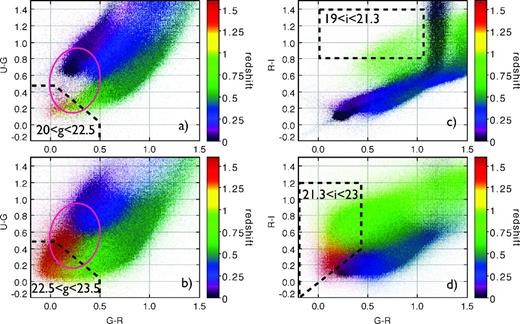
Colour–colour diagrams tinted according to the CFHT-LS photometric redshift. Colour selections are indicated with the dashed boxes. Quasars, when overlapping with the colour selection, are located in the pink ellipse. The stellar sequence appears in black. (a) The bright ugr colour selection: the u–g versus g–r diagram for 20 < g < 22.5. In this area the overall density of targets is low. (b) The faint ugr colour selection where the magnitude range is 22.5 < g < 23.5. The density of available targets increases and the stellar sequence is diminished. (c) The bright gri colour selection: the r–i versus g–r diagram for 19 < i < 21.3. The high-redshift targets are not as visible as in the ugr plot. The target density is also small. (d) The faint gri colour selection where the magnitude range is 21.3 < i < 23. The target density increases and higher redshift targets appear in the blue end of the colour plot while the stellar locus fades. Using SDSS photometry one would obtain similar plots to (a) and (c) in terms of target density.
COSMOS is a deep 2 deg2 survey that has been observed at more than 30 different wavelengths (Scoville et al. 2007). The COSMOS photometric catalogue is described in Capak et al. (2007) and the photometric redshifts in Ilbert et al. (2009). The COSMOS Mock Catalog (CMC9) is a simulated spectrophotometric catalogue based on the COSMOS photometric catalogue and its photometric redshift catalogue. The magnitudes of an object in any filter can be computed using the photometric redshift best-fitting spectral templates (Jouvel et al. 2009; Zoubian et al., in preparation).
The limiting magnitudes of the CMC in each band are the same as in the real COSMOS catalogue (detection at 5σ in a 3 arcsec diameter aperture): u < 26.4, g < 27, r < 26.8, i < 26.2. For magnitudes in the range 14 < m < 26 in the g, r and i bands from the Subaru telescope and in the u band from CFHT-LS, the CMC contains about 280 000 galaxies in 2 deg2 to COSMOS depth. The mock catalogue also contains a simulated spectrum for each galaxy. These simulated spectra are generated with the templates used to fit COSMOS photometric redshifts. Emission lines are empirically added using Kennicutt calibration laws (Kennicutt 1998; Ilbert et al. 2009), and have been calibrated using zCOSMOS (Lilly et al. 2009) as described in Zoubian et al. (in preparation). The strength of [O ii] emission lines was confirmed using DEEP2 and VVDS DEEP luminosity functions (Le Fèvre et al. 2005b; Zhu, Moustakas & Blanton 2009). Finally, a host galaxy extinction law is applied to each spectrum. Predicted observed magnitudes take into account the presence of emission lines.
3.2 Colour selections
Based on the COSMOS and CFHT-LS photometric redshifts, we explore two simple colour selection functions using the ugr and gri bands. Fig. 3 shows the targets available in the ugr and gri colour planes. We construct a bright and a faint sample based on the photometric depths of SDSS and CFHT-LS.
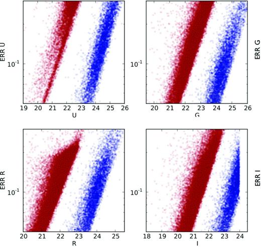
The four bands ugri and their precision are illustrated: in red for SDSS photometry and in blue for CFHT-LS photometry. The u-band quality is limiting the precision of the colour selection on SDSS photometry. Note that the photometric redshift CFHT-LS catalogue is cut at i = 24, and the SDSS data are R-selected with errR ≤ 0.2.
3.2.1 ugr selection
The ugr colour selection is defined by −1 < u − r < 0.5 and −1 < g − r < 1 that selects galaxies at z ≥ 0.6 and ensures that these galaxies are strongly star forming (u − r cut). The cut −1 < u − g < 0.5 removes all low-redshift galaxies (z < 0.3). Finally, the magnitude range is 20 < g < 22.5 and g < 23.5 for the bright and faint samples, respectively; see Figs 3(a) and (b).
3.2.2 gri selection
The bright gri colour selection is defined by the range 19 < i < 21.3. We select blue galaxies at z ∼ 0.8 with 0.8 < r − i < 1.4 and −0.2 < g − r < 1.1 (Fig. 3 c). In the faint range 21.3 < i < 23, we tilt the selection to select higher redshifts with −0.4 < g − r < 0.4, −0.2 < r − i < 1.2 and g − r < r − i (Fig. 3 d).
3.3 Predicted properties of the selected samples
The ugr colour selection avoids the stellar sequence, but not the quasar sequence. Hence, the contamination of the ugr selection by point-source objects is primarily due to quasars; see Figs 3(a) and (b). The resulting photometric redshift distribution as derived from the CFHT-LS photometric redshift catalogue has a wide span in redshift, covering 0.6 < z < 2 as shown in Fig. 4. The distribution is centred at z = 1.3 for the bright and the faint sample with a scatter of 0.3 (see Table 2). The expected [O ii] fluxes are computed from the CMC catalogue and are shown in Fig. 4. For 90 per cent of the galaxies in the faint sample, the predicted flux is above 10.6 × 10⁻¹⁷ erg cm−2 s−1. The bright sample galaxies show strong emission lines.
![Redshift and line flux distribution for various colour selections. The blue solid line is the ugr selection limited to 20 < g < 22.5. The blue dashed line is the ugr selection limited to 22.5 < g < 23.5. The red solid line is the gri selection limited to 19 < i < 21.3. The red dashed line is the gri selection limited to 21.3 < i < 23.0. Left: photometric redshift distribution from the CFHT-LS catalogue. Black solid line: no colour selection, but limited to i < 24. The ugr selection is more spread in redshift than the gri selection. The vertical dashed line indicates the upper limit of z = 1.7 that corresponds to [O ii] emission lines at ∼ 1 μm. Right: expected [O ii] flux distribution from the CMC simulation. The black solid line is the complete CMC catalogue. The ugr selection identifies stronger line emitters than the gri selection scheme. The vertical dashed line indicates the expected mean sensitivity of BOSS in 1 h exposure, 5 × 10⁻¹⁷ erg s−1 cm−2.](https://oup.silverchair-cdn.com/oup/backfile/Content_public/Journal/mnras/428/2/10.1093/mnras/sts127/2/m_sts127fig4.jpeg?Expires=1749873944&Signature=DjULlxmJstHfbHMuZL-DegXkQyoSBMfDshLZud2xALp691hRhXwoW4mpN7AIWFCb~2EHWiyF13v36XWqnJelHwH~mc6mXgfDEgz5n00ckxSKJsD34EDRW-WU-hxFJcYgKqJajermiEVIJeDwhWEUDuN6eT4WSrU7JLzHC2mlDEcblKrpztzLY3pztrDd7Y-AAo1mjXKcB1ZQiHrCsU5TCBK5QU~AlS8ZmeGADyVRVU9HJMtakjNHcIiyeMUbBLdpdzurMTKd1q3WvLrswZIQSTaDIEHHM8hk41McER0CmyuHywuERfJ-ioRibvwWRc7je8RFlC~I0Um9P0TEWqAhhA__&Key-Pair-Id=APKAIE5G5CRDK6RD3PGA)
Redshift and line flux distribution for various colour selections. The blue solid line is the ugr selection limited to 20 < g < 22.5. The blue dashed line is the ugr selection limited to 22.5 < g < 23.5. The red solid line is the gri selection limited to 19 < i < 21.3. The red dashed line is the gri selection limited to 21.3 < i < 23.0. Left: photometric redshift distribution from the CFHT-LS catalogue. Black solid line: no colour selection, but limited to i < 24. The ugr selection is more spread in redshift than the gri selection. The vertical dashed line indicates the upper limit of z = 1.7 that corresponds to [O ii] emission lines at ∼ 1 μm. Right: expected [O ii] flux distribution from the CMC simulation. The black solid line is the complete CMC catalogue. The ugr selection identifies stronger line emitters than the gri selection scheme. The vertical dashed line indicates the expected mean sensitivity of BOSS in 1 h exposure, 5 × 10⁻¹⁷ erg s−1 cm−2.
The gri selection avoids both the stellar sequence and the quasar sequence; see Figs 3(c) and (d). Thus, the contamination from point sources should be minimal. Fig. 4 shows the photometric redshift distribution of the gri selection applied to CFHT photometry. The redshifts are centred at z = 0.8 for the bright and z = 1.0 for the faint sample (see Table 2). The expected [O ii] flux, computed with the CMC catalogue, is shown in Fig. 4. Emissions are weaker than for the ugr selection as expected.
The different selections shown in Figs 3 and 4 are summarized in Table 2, which contains the number densities available, mean magnitudes, mean redshifts and mean [O ii] fluxes (when available) of the different samples considered. We have lower densities in the CMC than in the CFHT-LS catalogue. This is probably due to cosmic variance as the CMC only covers 2 deg2.
Properties of the colour-selected samples. ‘b’ stands for bright (20 < g < 22.5 for ugr or 19 < i < 21.3 for gri) and ‘f’ stands for faint (22.5 < g < 23.5 for ugr or 21.3 < i < 23 for gri). We indicate the mean and standard deviation of the redshift distribution for each set. For the CMC sample, [O ii] fluxes are expressed in units of 10−17 erg cm−2 s−1; the median, the first and third quartiles of the flux distribution are indicated. The ugr tends to select the highest [O ii] fluxes.
| Selection | No.deg− 2 | |$\bar{u}$| | |$\bar{g}$| | |$\bar{r}$| | |$\bar{i}$| | |$\bar{z}$| | σz | |$\bar{f}_{\left[\mathrm{O\,{\rm II}}\right]}$| | |$Q^1_{f_{\left[\mathrm{O\,{\rm II}}\right]}}$| | |$Q^3_{f_{\left[\mathrm{O\,{\rm II}}\right]}}$| | ||
|---|---|---|---|---|---|---|---|---|---|---|---|---|
| CMC | ugr | b | 130.0 | 21.98 | 21.87 | 21.69 | – | 1.25 | 0.53 | 61.74 | 46.47 | 88.39 |
| f | 1450.8 | 23.27 | 23.18 | 22.98 | – | 1.19 | 0.38 | 16.60 | 13.06 | 22.26 | ||
| gri | b | 257.2 | – | 22.69 | 21.87 | 20.93 | 0.80 | 0.21 | 13.85 | 8.65 | 22.21 | |
| f | 2170.5 | – | 23.34 | 23.09 | 22.55 | 0.93 | 0.31 | 10.23 | 6.83 | 15.99 | ||
| CFHT-W1 | ugr | b | 193.3 | 21.95 | 21.8 | 21.7 | – | 1.28 | 0.38 | |||
| f | 1766.8 | 23.37 | 23.19 | 23.07 | – | 1.29 | 0.31 | |||||
| gri | b | 361.4 | – | 22.62 | 21.8 | 20.82 | 0.81 | 0.11 | ||||
| f | 3317.5 | – | 23.34 | 23.11 | 22.55 | 1.03 | 0.35 | |||||
| CFHT-W3 | ugr | b | 232.2 | 21.89 | 21.76 | 21.69 | – | 1.27 | 0.37 | |||
| f | 1679.1 | 23.36 | 23.18 | 23.06 | – | 1.28 | 0.31 | |||||
| gri | b | 391.6 | – | 22.62 | 21.78 | 20.8 | 0.82 | 0.1 | ||||
| f | 3334.2 | – | 23.34 | 23.11 | 22.54 | 1.03 | 0.33 | |||||
| SDSS | ugr | b | 166.96 | 21.76 | 21.77 | 21.52 | – | |||||
| gri | b | 204.96 | – | 22.57 | 21.75 | 20.76 | ||||||
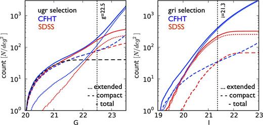
The SDSS colour-selected samples are complete for the bright samples at g < 22.5 and i < 21.3, not for the faint samples. The CFHT-LS-selected samples are complete for both the bright and faint samples; see Fig. 5, where the total cumulative number counts (solid line) of the ugr and gri colour-selected samples are plotted as a function of g and i bands, respectively. On the bright end of this figure, although both photometries are complete at the bright limit, we note a discrepancy between the total amount of targets selected on CFHT and SDSS that implies selections on CFHT are denser than on SDSS (difference between the red and blue solid lines). This is due to the transposition of the colour selection from one photometric system to the other. In fact, we select targets on SDSS with a transposed criterion from CFHT using the calibrations by Regnault et al. (2009). The transposed criterion is as tight as the original. But as the errors on the magnitude are larger in the SDSS system, their colour distributions are more spread. Therefore, the SDSS selection is a little less dense than the CFHT selection.
Targeting the bright range is limited by galaxy density; in the best case, one can reach 300 targets deg−2 and contains point sources (stars and quasars) and low-redshift galaxies. In the faint range, the target density is 10 times greater, but the exposure time necessary to assign a reliable redshift will be much longer (1 mag deeper for a continuum-based redshift roughly corresponds to an exposure five times longer). The stellar, quasars and low-redshift contamination is smaller in the faint range. Fig. 4 shows the distributions in redshift and in [O ii] flux we expect given a magnitude range and a colour criterion within the framework of the CMC simulation. The main trend is that the ugr selection identifies strong [O ii] emitters out to z ∼ 2 where the gri peaks at z = 1 and extends to 1.4 with weaker [O ii] emitters.
We also used a criterion to split targets in terms of compact and extended sources, which is illustrated in Fig. 5. For CFHT-LS we have used the half-light radius (r2 value, to be compared to the rlimit2 value which defines the maximal size of the point spread function at the location of the object considered – see Coupon et al. 2009 and CFHT-LS T0006 release document) to divide the sample into compact and extended objects. For SDSS we used the ‘type’ flag, which separates compact (type=6) from extended objects (type=3). For the ugr colour selection, the number counts are dominated by compact blue objects (quasars) at g ≤ 22.2. At g ≥ 22.2, the counts are dominated by extended ELGs. For comparison, we show in Fig. 5 the cumulative counts of the XDQSO catalogue from Bovy et al. (2011) who identified quasars in the SDSS limited to g < 21.5. We note an excellent match with the bright (compact) ugr colour-selected objects. For the gri colour selection, there is a low contamination by compact objects because the colour box does not overlap with either the stellar or the quasar sequence.
Cumulative number counts per square degree of both colour selections using SDSS photometry (in red) and CFHT-LS photometry (in blue). The solid line is the whole selection, while the dashed line is for compact (star-like) objects and the dotted line represents extended objects. On the left is the ugr selection and on the right is the gri selection. The black dashed line represents objects from the XDQSO catalogue that have a probability of being a quasar that is greater than 90 per cent (Bovy et al. 2011) (the quasar identifications are limited to g = 21.5).
4 ELG OBSERVATIONS
To test the reliability of both the bright ugr (g < 22.5) and the bright gri (i < 21.3) colour selections, we have conducted a set of dedicated observations, as part of the ‘Emission Line Galaxy SDSS-III/BOSS ancillary programme’. The observations were conducted between Autumn 2010 and Spring 2011 using the SDSS telescope with the BOSS spectrograph at Apache Point Observatory. A total of ∼2000 spectra, observed four times for 15 min, were taken in different fields, namely in the Stripe-82 (using single-epoch SDSS photometry for colour selection) and in the CFHT-LS W1, W3 and W4 wide fields (using CFHT-LS photometry). This data set was released in the SDSS-III Data Release 9.10
4.1 Description of SDSS-III/BOSS spectra
We used the SDSS photometric catalogue (Aihara et al. 2011) to select 313 objects according to their ugr colours located in the Stripe-82 and 899 objects selected according to their gri colours in the CFHT-LS W3 field. In addition, we used the CFHT-LS photometry to select 878 ugr targets in the CFHT-LS W1 field and 391 gri targets in the CFHT-LS W3 field for observation. The spectra are available in the SDSS Data Release 9 and flagged ‘ELG’.
All of these spectra were manually inspected to confirm or correct the redshifts produced by two different pipelines (zcode and its modified version that we used to fit the [O ii] emission-line doublet). As the BOSS pipeline redshift measurement is designed to fit LRG continuum, some ELGs with no continuum were assigned wrong redshifts. To classify the observed objects, we have defined seven subcategories.
Objects with secure redshifts
‘ELG’, emission-line galaxy (redshift determined with multiple emission lines). Usually, these spectra have a weak ‘blue’ continuum and lack a ‘red’ continuum. Empirically, using platefit vimos pipeline output, this class corresponds to a spectrum with more than two emission lines with observed equivalent widths EW ≤ −6 Å; see examples in Appendix A and Figs A1, A2 and A3.
‘RG’, red galaxy with continuum in the red part of its spectrum, allowing a secure redshift measurement through multiple absorption lines (e.g. Ca K&H, Balmer lines) and the 4000 Å break. Some of these objects have also weak emission (E+A galaxies). Empirically their spectra have a mean Dn(4000) of 1.3, where Dn(4000) is the ratio of the continuum level after the break and before the break. These galaxies typically have i ∼ 20, which is fainter than the CMASS targeted by BOSS.
‘QSO’, quasars, which are identified through multiple broad lines. Examples are given in Fig. A4.
Stars.
Objects with unreliable redshifts
‘Single emission line’: the spectra contain only a single emission line which cannot allow a unique redshift determination. For this population, the CFHT T0006 photometric redshifts are compared to the [O ii] redshift (assuming that the single emission line is [O ii]) in Fig. 6. The two estimates agree very well: 77.7 per cent have (zspec − zphot)/(1 + zspec) < 0.1 for the gri selection and 62.7 per cent for the ugr selection. These galaxies with uncertain redshift tend to have slightly fainter magnitudes with a mean CFHT g magnitude at 22.6 and a scatter of 0.6, whereas for the whole ELGs is 22.4 with a scatter of 0.4.
‘Low continuum’ spectra that show a 4000 Å break too weak for a secure redshift estimate. The agreement between photometric and spectroscopic redshift estimation is excellent: 84.6 per cent within 10 per cent errors; see Fig. 6.
‘Bad data’, the spectrum is either featureless, extremely noisy or both.
The detailed physical properties of the ELGs are discussed in Section 5 and a number of representative spectra are displayed in Appendix A.
![T0006 CFHT-LS photometric redshifts of single emission line and low continuum galaxies observed against [O ii] redshift. A strong correlation is clearly evident. A slight systematic overestimation of the photometric redshift is visible above z = 1.2 (these photometric redshifts were calibrated below z = 1.2).](https://oup.silverchair-cdn.com/oup/backfile/Content_public/Journal/mnras/428/2/10.1093/mnras/sts127/2/m_sts127fig6.jpeg?Expires=1749873944&Signature=YsP1~3c8oLwQ-BRO33Sk99MlxyMG3KvnEruwK-unC9QIajxNN3y0lIK82AWOflR3EBgB5ChqaX6zWgQQGqvGLCWKK-nkUNfwYlmRsqc3QSvw3CyWLbrTapgmIKG8C~d9kcxLTZE~vKuSDG57-05K8yLkWlVFBUZc8Qdet5GcDC1sfCrjrDQq14l2YzLaJhRIDLP1QfQFySGOkL09v1Et5S91X778c9nCT4KyK9FDSbQuh8d37bAwQ3cKMVKK~qKv0nbuV8Us4UJlAI4BLp7TL6AHqekqrNYZv2uhlfB5DnEiskpURZRAS~DKfHzF0ewHfbp23DCmel0z61OOv6LXzQ__&Key-Pair-Id=APKAIE5G5CRDK6RD3PGA)
T0006 CFHT-LS photometric redshifts of single emission line and low continuum galaxies observed against [O ii] redshift. A strong correlation is clearly evident. A slight systematic overestimation of the photometric redshift is visible above z = 1.2 (these photometric redshifts were calibrated below z = 1.2).
4.2 Redshift identification
The results of the observations are summarized by categories in Table 3.
Observed objects split in categories.
| gri selection | ugr selection | |||||||
|---|---|---|---|---|---|---|---|---|
| SDSS selection | CFHT-LS selection | SDSS selection | CFHT-LS selection | |||||
| Type | Number | Per cent | Number | Per cent | Number | Per cent | Number | Per cent |
| ELG (z > 0.6) | 450 | 50 | 240 | 61 | 100 | 32 | 402 | 46 |
| ELG (z < 0.6) | 60 | 7 | 3 | 1 | 101 | 32 | 84 | 9 |
| RG (z > 0.6) | 73 | 8 | 46 | 12 | 0 | 0 | 0 | 0 |
| RG (z < 0.6) | 30 | 3 | 0 | 0 | 7 | 3 | 0 | 0 |
| Single emission line | 36 | 4 | 12 | 3 | 0 | 0 | 102 | 12 |
| Low continuum | 13 | 1 | 1 | 0 | 0 | 0 | 0 | 0 |
| QSO | 8 | 1 | 5 | 1 | 30 | 10 | 126 | 14 |
| Stars | 44 | 5 | 12 | 3 | 10 | 3 | 6 | 1 |
| Bad data | 185 | 21 | 72 | 18 | 65 | 20 | 158 | 18 |
| Total | 899 | 100 | 391 | 100 | 313 | 100 | 878 | 100 |
For the targets selected using SDSS photometry and with the ugr selection, 32 per cent are ELGs at z > 0.6 (100 spectra). The low-redshift ELGs represent 32 per cent of the observed targets (101 spectra). The other categories are 65 ‘bad data’ (20 per cent), 30 quasars (10 per cent), 10 stars (3.5 per cent) and seven red galaxies with z < 0.6 (2.5 per cent). With the gri selection, 57 per cent of the targets are at z > 0.6. However, still 21 per cent of the spectra fall into the bad data class.
Using CFHT-LS photometry, 46 per cent of the targets are ELGs at z > 0.6 and 14 per cent are quasars with the ugr selection. With the gri selection, 73 per cent are galaxies at z > 0.6, five-sixths of which are ELGs.
For both selections, targeting with CFHT-LS is more efficient than with SDSS. The complete classification of observed targets is given in Table 3. The redshift distribution of the observed objects is compared to the distributions from the BOSS and WiggleZ current BAO experiments in Fig. 7. The figure shows that ugr and gri target selections enable a BAO study at higher redshifts. With a joint selection, we can reach the requirements described in Table 1 to detect BAO feature to z = 1.
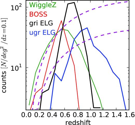
Observed redshift distribution for the ugr ELGs (blue), the gri ELGs (black) compared to the distribution of galaxies from BOSS (red) and WiggleZ (green). Magenta lines represent constant density of galaxies at 1 and 3 × 10⁻⁴ h3 Mpc−3, it constitutes our density goals.
4.3 Comparison of measured ELGs with the CMC forecasts
To investigate the expected purity of ELG galaxy samples, we created mock catalogues covering redshifts between 0.6 and 1.7. Continuum spectra of ELGs were generated from the CMC and emission lines were added according to the modelling described in Jouvel et al. (2009). Two simulated galaxy catalogues were built, one for each colour selection function (ugr and gri). Each synthetic spectrum was affected by sky and photon noise as if observed by BOSS spectrographs, by using the specsim1d software. We simulated a set of four exposures of 900 s each. The resulting simulated spectra were then analysed by the zcode pipeline (Cannon et al. 2006) to extract the spectroscopic redshift. As our targets are mainly ELGs, we only use the redshift estimate based on fitting discrete emission-line templates in Fourier space over all z.
We address the flux measurement of emission lines. This exercise was conducted using the platefit vimos software developed by Lamareille et al. (2009). This software is based on the platefit software that was developed to analyse SDSS spectra (Brinchmann et al. 2004; Tremonti et al. 2004). The platefit vimos software was developed to measure the flux of all emission lines after removing the stellar continuum and absorption lines from lower resolution and lower signal-to-noise ratio spectra (Lamareille et al. 2006). The stellar component of each spectrum is fit by a non-negative linear combination of 30 single stellar population templates with different ages (0.005, 0.025, 0.10, 0.29, 0.64, 0.90, 1.4, 2.5, 5 and 11 Gyr) and metallicities (0.2, 1 and 2.5 Z⊙). These templates have been derived using the Bruzual & Charlot (2003) libraries and have been resampled to the velocity dispersion of VVDS spectra. The dust attenuation in the stellar population model is left as a free parameter. Foreground dust attenuation from the Milky Way has been corrected using the Schlegel, Finkbeiner & Davis (1998) maps.
After removal of the stellar component, the emission lines are fit as a single nebular spectrum made of a sum of Gaussians at specified wavelengths. All emission lines are set to have the same width, with the exception of the |$\left[\mathrm{O\,{\rm II}}\right]\lambda 3727$| line which is a doublet of two lines at 3726 and 3729 Å that appear broadened compared to other single lines. Detected emission lines may also be removed from the original spectrum in order to obtain the observed stellar spectrum and measure indices, as well as emission-line equivalent widths. The underlying continuum is obtained by smoothing the stellar spectrum. Equivalent widths are then measured via direct integration over a 5σ bandpass of the emission-line Gaussian model divided by the underlying continuum. Then emission-line fluxes are measured for each simulated spectra using the extracted redshift from zcode and the true redshift for cross-checks.
We consider that a redshift has been successfully measured if Δz/(1 + z) < 0.001. We believe that this threshold could be lowered to 10−4 in the future by using a more advanced redshift solver. Using the current pipeline, we can distinguish these two regimes.
The first regime is the redshift range z < 1.0. Many emission lines ([O ii], Hβ, [O iii]) are present in the SDSS spectrum. For g < 23.5, 91 per cent of the redshifts are measured successfully. Among the remaining 9 per cent, catastrophic failures represent 3.5 per cent [the pipeline outputs a redshift between 0 and 1.6 with Δz/(1 + z) > 0.01]. Inaccurate redshifts represent 3.9 per cent [the pipeline outputs a redshift between 0 and 1.6 with 0.001 < Δz/(1 + z) < 0.01] and 1.5 per cent are not found by the pipeline (z = −9 is output).
The second regime is the redshift range 1.0 ≤ z < 1.7: the redshift determination hinges on the identification of the [O ii] doublet. For g < 23.5, 66.8 per cent of the redshifts are measured successfully. 19.1 per cent are catastrophic failures and 14.1 per cent are inaccurate redshifts. Work is ongoing to improve the redshift measurement efficiency at z > 1. In the second regime, the minimum [O ii] flux required to compute a reliable redshift depends on the redshift/wavelength because of the strong OH sky lines in the spectrum. We infer from the observed spectra that to measure a reliable redshift, we require a 5σ detection of the [O ii] lines, which means a (blended or not) detection of two peaks in the emission line separated by 2(1 + z). The detection significance is defined from the 1D spectrum. From the data the faintest 5σ detections are made with a flux of 4 × 10⁻¹⁷ erg s−1 cm−2 and the brightest 5σ detections need a flux of 2 × 10⁻¹⁶ erg s−1 cm−2 to be on the top of sky lines. The simulation shows the same thresholds; see Fig. 8. The simulation confirms the detection limit we observe. The bottom plot of Fig. 8 raises the issue that the sky time variation has a non-negligible impact on the detection limit of the [O ii] emission doublet for redshifts z > 1.1. Though this ELG sample is too small to address this issue. In fact, the sample was observed during 10 different nights and the number of ELGs with z > 1.1 is less than 60. It is thus not possible to derive a robust trend comparing the [O ii] detections to the sky value of each observation. Handling this issue would require a sample of ∼500 redshifts in the range 1.1 < z < 1.6 observed many times over many nights. With such a sample in hand, we could quantify exactly how to optimize the observational strategy.
![Top: flux detected in the [O ii] doublet (green or red filled circle for a simulated spectrum and blue filled square for a real galaxy observation) versus redshift. The simulation is coloured according to the measured line flux divided by the error. The black solid line represents a typical sky as observed by BOSS spectrograph; the 5σ detections of [O ii] follow the sky flux. The [O ii] detections above 5σ (red circles) follow the tendency of the sky fluctuations: a 5σ detection in a zone with a high sky requires a larger emitted flux. The data are scaled to match a 1 h exposure on the 2.5-m SDSS telescope. The redshifts below the sky flux are assigned using other emission lines or the information in the continuum. Bottom: an expansion of the top panel using z > 1 detections. Only measured galaxies are plotted upon the mean sky (black) and the best sky (red) of Apache Point Observatory (APO).](https://oup.silverchair-cdn.com/oup/backfile/Content_public/Journal/mnras/428/2/10.1093/mnras/sts127/2/m_sts127fig8.jpeg?Expires=1749873944&Signature=FXJSy0U49clRowhtKnKzmwTjkMyIESeR8JOX8dl98gD9Ay7sapE5QLzHA3kxmsEbVQhApiG~ZCfTngtZChQ3LY1s6B652jybLlmTjlaBtaN45olAXp~D3bWBTTWBJm8f34IvyWZTux0VUZt7vQhfYrnLuCH4--wB6ni1RMhBsfLhaOm0l3FG6KaZiXOrirLwEXjeineiaKTGezO2mcdbYH4tVCnkuWsYJWjYsDpAOss0Mm0uIXQydahwh-T~9FKZuvDW9PU8-iFBdiw4rESZQEM5R8OtVxbJAj8hzsqOUqHZZRkpIrrSsz7cK5nVdWtUTFo36ouTTMLQKLoH7KUBKQ__&Key-Pair-Id=APKAIE5G5CRDK6RD3PGA)
Top: flux detected in the [O ii] doublet (green or red filled circle for a simulated spectrum and blue filled square for a real galaxy observation) versus redshift. The simulation is coloured according to the measured line flux divided by the error. The black solid line represents a typical sky as observed by BOSS spectrograph; the 5σ detections of [O ii] follow the sky flux. The [O ii] detections above 5σ (red circles) follow the tendency of the sky fluctuations: a 5σ detection in a zone with a high sky requires a larger emitted flux. The data are scaled to match a 1 h exposure on the 2.5-m SDSS telescope. The redshifts below the sky flux are assigned using other emission lines or the information in the continuum. Bottom: an expansion of the top panel using z > 1 detections. Only measured galaxies are plotted upon the mean sky (black) and the best sky (red) of Apache Point Observatory (APO).
5 PHYSICAL PROPERTIES OF ELGs
All ugr and gri ELG spectra were analysed with two different software packages: the platefit vimos (Lamareille et al. 2009) and the Portsmouth Spectroscopic Pipeline (Thomas et al. 2012). In this section we discuss the following physical properties of the observed ELGs: redshift, star-forming rate (SFR), stellar mass, metallicity and classification of the ELG type [Seyfert 2, low-ionization nuclear emission-line regions (LINERs), SFG, composite]. To estimate how these quantities vary over time, and with their environment, observations of larger samples of ELGs are planned. Future sample will allow us to estimate how the clustering of the galaxies depends on these physical quantities. It is key to replace future BAO tracers in the galaxy formation history. With the current sample, we draw simple trends using means and standard deviation of the observed quantities, and we place the ELGs in the galaxy classification made by Lamareille (2010) and Marocco, Hache & Lamareille (2011).
5.1 Main properties
The main properties of the ELGs are shown in Table 4. The SFR was computed using equation (18) of Argence & Lamareille (2009). The stellar mass was estimated using the CFHT-LS ugriz photometry. (The errors on the stellar mass using only SDSS photometry were too large to be meaningful, thus the empty cells in the table.) The metallicity is estimated using the calibration by Tremonti et al. (2004). The main trends are as follows.
Main properties of the observed galaxies. Fluxes are in unit of 10−17 erg cm−2 s−1. Equivalent widths ‘EW’ are in Å.
| gri-selected ELG | ugr-selected ELG | |||||||
|---|---|---|---|---|---|---|---|---|
| CFHT-LS | SDSS | CFHT-LS | SDSS | |||||
| Mean | σ | Mean | σ | Mean | σ | Mean | σ | |
| EW|$_{\left[\mathrm{O\,{\rm II}}\right]}$| | −14.86 | 9.01 | −16.75 | 10.13 | −50.58 | 27.24 | −30.75 | 23.04 |
| Flux|$_{\left[\mathrm{O\,{\rm II}}\right]}$| | 16.85 | 9.65 | 18.58 | 10.37 | 30.36 | 30.1 | 24.23 | 39.27 |
| EWHβ | −10.28 | 10.8 | −10.72 | 8.65 | −24.27 | 22.88 | −17.18 | 19.34 |
| FluxHβ | 15.44 | 8.6 | 14.63 | 7.72 | 12.97 | 15.16 | 12.57 | 23.91 |
| EW|$_{\rm III}$| | −10.09 | 10.98 | −11.33 | 10.76 | −65.3 | 91.56 | −16.89 | 30.49 |
| Flux|$_{\rm III}$| | 17.74 | 20.15 | 17.43 | 21.59 | 35.13 | 53.49 | 13.39 | 37.79 |
| 12 + log OH | 8.94 | 0.20 | 8.92 | 0.19 | 8.69 | 0.21 | 8.69 | 0.25 |
| log SFR|$_{\left[\mathrm{O\,{\rm II}}\right]}$| | 0.97 | 0.35 | 0.92 | 0.45 | 0.96 | 1.24 | 0.76 | 0.84 |
| log (M*/M⊙) | 10.85 | 0.3 | 10.23 | 6.87 | 9.33 | 0.80 | – | – |
The gri-selected galaxies of CFHT-LS are the more massive galaxies in terms of stellar mass.
The ugr selects stronger SFGs than gri (due to the u-band selection). There is a factor of 2 variation in the strength of the measured oxygen lines.
The ugr selects galaxies that have 12 + log [OH] ∈ [8, 9], whereas gri focuses slightly more on the higher, i.e. 12 + log [OH] ≈ 9.
The SFR appears to be independent of the colour selection schemes.
5.2 Classification
We use a recent classification (Lamareille 2010; Marocco et al. 2011) for the ELG sample. The classification is made using |$\log (\left[\mathrm{O\,{\rm III}}\right]/{\rm H}\beta )$|, |$\log (\left[\mathrm{O\,{\rm II}}\right]/{\rm H}\beta )$|, Dn(4000) and |$\log [{\rm max}({\rm EW}_{\left[\mathrm{O\,{\rm II}}\right]},{\rm EW}_{\left[\mathrm{Ne\,{\rm III}}\right]})]$|. We compare the ELG sample to zCOSMOS, as zCOSMOS has numerous SFGs in the redshift range we are observing. Fig. 9(a) shows that the zCOSMOS and the ugr ELG samples are located in three of the five areas delimited by the classification: Seyfert 2 (‘Sy2’), ‘SFGs’ and a third region where both mix (‘Sy2/SFG’). There are a few LINERs and Composite in either sample. Fig. 9(b) separates the ugr galaxies in the ‘Sy2/SFG’ area into ‘SFG’ or ‘Sy2’, and shows that zCOSMOS galaxies from the ‘Sy2/SFG’ area are both ‘Sy2’ and ‘SFG’ where the ugr ELGs in the ‘Sy2/SFG’ area are mostly ‘SFG’. The gri-observed sample is located in the area of ‘SFGs’, whether one considers the one selected on CFHT or on SDSS. Finally, the ELG selected, ugr or gri, are both in the ‘SFG’ part of the classification.
![Black dots stand for CFHT-LS-selected ELGs, red dots for SDSS-selected ELGs and grey contours or grey pixels for zCOSMOS survey galaxies. (a) $\log (\left[\mathrm{O\,{\rm III}}\right]/{\rm H}\beta )$ versus $\log (\left[\mathrm{O\,{\rm II}}\right]/{\rm H}\beta )$ for ugr ELGs. The ugr ELG sample is located in a similar area than zCOSMOS galaxies. (b) Dn(4000) versus $\log [{\rm max}({\rm EW}_{\left[\mathrm{O\,{\rm II}}\right]},{\rm EW}_{\left[\mathrm{Ne\,{\rm III}}\right]})]$ for ugr ELGs. Only galaxies from the ‘Sy2/SFG’ area from the plot (a) are represented. The ugr ELG is thus mainly composed of ‘SFG’. (c) $\log (\left[\mathrm{O\,{\rm III}}\right]/{\rm H}\beta )$ versus $\log (\left[\mathrm{O\,{\rm II}}\right]/{\rm H}\beta )$ for gri ELGs. The gri ELG sample is located in the ‘SFG’ area.](https://oup.silverchair-cdn.com/oup/backfile/Content_public/Journal/mnras/428/2/10.1093/mnras/sts127/2/m_sts127fig9.jpeg?Expires=1749873944&Signature=qEP0OEfKCFGZqhe8lSRGOVoorXDzPBtnkLHVBNxO~XCm~r65VEeB6qhmpWOBxRZ8vgs7B8cylakDYxEH-fcJd6a~vcLZ0UDYRuN6QHn225roS4lnX2JrnjQ9kOt4l7TgcGKG4AzfJG0rzcsmDiuu0KfPEuvBincZt1NhK5x6Lb5KHe~wnLjSbxgevqi4-Xil3gYUA~z6ByA1BMgT9~TcsdBScmNXNa9aYOCDe7~jOTJ96f4o0xv2cmfu5sekJwQxrXmdE51r8sGUN8UDNxqIeleg3x4UzgW4cCJTuuyDkvhI5YyTJoro9UC07S655wilcYvejajvdh1h-JDGPwB-~Q__&Key-Pair-Id=APKAIE5G5CRDK6RD3PGA)
Black dots stand for CFHT-LS-selected ELGs, red dots for SDSS-selected ELGs and grey contours or grey pixels for zCOSMOS survey galaxies. (a) |$\log (\left[\mathrm{O\,{\rm III}}\right]/{\rm H}\beta )$| versus |$\log (\left[\mathrm{O\,{\rm II}}\right]/{\rm H}\beta )$| for ugr ELGs. The ugr ELG sample is located in a similar area than zCOSMOS galaxies. (b) Dn(4000) versus |$\log [{\rm max}({\rm EW}_{\left[\mathrm{O\,{\rm II}}\right]},{\rm EW}_{\left[\mathrm{Ne\,{\rm III}}\right]})]$| for ugr ELGs. Only galaxies from the ‘Sy2/SFG’ area from the plot (a) are represented. The ugr ELG is thus mainly composed of ‘SFG’. (c) |$\log (\left[\mathrm{O\,{\rm III}}\right]/{\rm H}\beta )$| versus |$\log (\left[\mathrm{O\,{\rm II}}\right]/{\rm H}\beta )$| for gri ELGs. The gri ELG sample is located in the ‘SFG’ area.
6 DISCUSSION
6.1 Redshift identification rates in ugr and gri
We summarize the redshift measurement efficiency of the gri and ugr colour-selected galaxies presented in this paper in Tables 3 and 5, and compare the results with those of WiggleZ (Drinkwater et al. 2010), BOSS and VIPERS (the percentages about VIPERS are based on a preliminary subset including only ∼20 per cent of the survey). The original VIPERS selection flag (J. Coupon & O. Ilbert, private communication) is defined to have colours compatible with an object at z > 0.5 if it has (r − i ≥ 0.7 and u − g ≥ 1.4) or [r − i ≥ 0.5(u − g) and u − g < 1.4] (Guzzo et al., in preparation). The efficiencies in Table 5 show that a better photometry and thus more precise colours yield a better efficiency in terms of obtaining objects in the targeted redshift range. It also shows that the colour selections proposed in this paper are competitive for building an LSS sample.
Redshift efficiency in per cent. Column 2 quantifies the amount of spectroscopic redshift obtained with the selection. Column 3 is the number of spectroscopic redshifts that are in the range the survey is aiming at; it is the efficiency of the target selection. The redshift window for ELG selection is z > 0.6.
| Selection | Spectroscopic | Object in | Quasars |
|---|---|---|---|
| scheme | redshift | z window | |
| gri SDSS | 80 | 62 | 1 |
| gri CFHT-LS | 82 | 73 | 1 |
| ugr SDSS | 80 | 32 | 10 |
| ugr CFHT-LS | 78 | 56 | 13 |
| WiggleZ | 60 | 35 | – |
| BOSS | 95 | 95 | – |
| VIPERS | 80 | 70 | – |
| Selection | Spectroscopic | Object in | Quasars |
|---|---|---|---|
| scheme | redshift | z window | |
| gri SDSS | 80 | 62 | 1 |
| gri CFHT-LS | 82 | 73 | 1 |
| ugr SDSS | 80 | 32 | 10 |
| ugr CFHT-LS | 78 | 56 | 13 |
| WiggleZ | 60 | 35 | – |
| BOSS | 95 | 95 | – |
| VIPERS | 80 | 70 | – |
To determine the necessary precision on the photometry to stay at the efficiencies observed, we degrade the photometry of the observed ELGs, then reselect them and recompute the efficiencies. Using a photometry less precise than the CFHT-LS by a factor of 2.5 in the errors (the ratio of the median values of the magnitude errors in bins of 0.1 mag equals 2.5) does not significantly change either the efficiency or the redshift distribution implied by the colour selection. This change also corresponds to loosening the colour criterion by 0.1 mag. For the eBOSS survey, a photometry 2.5 times less precise than CFHT-LS should be sufficient to maintain a high targeting efficiency (for comparison, SDSS is 10 times less precise than CFHT-LS); Fig. 10 shows the smearing of the galaxy positions in the colour–colour plane for a degraded photometry.
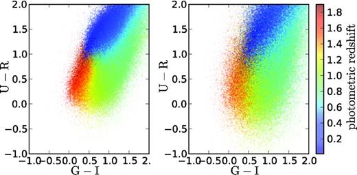
U − R versus G − I coloured according to the photometric redshift. Left: CFHT-LS photometry; Right: CFHT-LS photometry degraded by a factor of 2.5. This comparison shows how the degradation of the photometry smears the clean separations between galaxy populations in redshift.
6.2 Measurement of the |$[\mathrm{O\,{\rm II}}]$| doublet, single emission-line spectra
For ground-based spectroscopic surveys observing ELGs with 1 < z < 1.7, the only emission line remaining in the spectrum to assign the spectroscopic redshift is the [O ii] doublet. For the redshift to be certain, the doublet must be split (i.e. we do not want the target to be classified as ‘single emission line’ ELG). Fig. 11 shows a subsample of the observed bright ugr ELGs where [O ii] doublets are well resolved.
![Observed spectra zoomed on the [O ii] doublet, extracted from the ugr ELG sample. The doublet is split enough (apart from a little blending) to assign the correct spectroscopic redshift without the help of other emission lines.](https://oup.silverchair-cdn.com/oup/backfile/Content_public/Journal/mnras/428/2/10.1093/mnras/sts127/2/m_sts127fig11.jpeg?Expires=1749873944&Signature=m56LJ~E6-qb7dtvXis0I2q3tdqKtqBr6YQBQI9EltVmCxe5CKVzE-v97E0WmbgwfrD24CzAkn5iPdtOEBMu69GdJbd9vlJ8Oe47Jdg52i9clf4GfnhQZiV39sH1GIjEffe-hEk-YmqbFWUfQeJPl4GTROGJwG3r8-VT1KbsfxLN4DH~GOPuXcQD1nle~BESHgXdgxbX9o3cTNZAnqIgxOwf6AUvyzo0Lxs4efqV11V7vkilldTotN2L9hWXZ9UQHqadEAzAMlhtw7h0jLxqzFAqbmf~5bJLVN-ln8rRenB0M8YyUAlSqNUzxfN0ozLxuDhEVpLmKTuR1yg7QODJmxQ__&Key-Pair-Id=APKAIE5G5CRDK6RD3PGA)
Observed spectra zoomed on the [O ii] doublet, extracted from the ugr ELG sample. The doublet is split enough (apart from a little blending) to assign the correct spectroscopic redshift without the help of other emission lines.
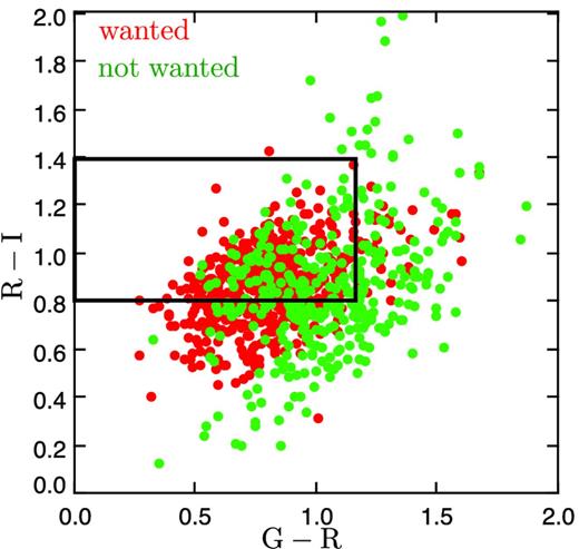
gri selection based on colours from SDSS (black box) represented on CFHT-LS magnitudes. The scatter is quite large: about half the targets would not have been selected if we used CFHT-LS photometry. The ‘wanted’ objects are galaxies at z > 0.6 or quasars and ‘unwanted’ objects are the rest.
![Photometric redshift distributions obtained using the ugri bands. The dashed black lines are the low- and high-density goals mentioned in Section 2, $\bar{n}=10^{-4}$ and 3 × 10⁻⁴ h3 Mpc−3. The dashed red line is the BOSS CMASS sample. The solid blue line is the distribution enhanced by the ugri selection, it has a projected sky density of ∼340 deg−2. The solid red line is the gri selection (projected sky density ∼350 deg−2). The solid green line is the ugr selection (projected sky density ∼400 deg−2). It shows the possibility of making a selection able to sample [0.6, 1.2] for a BAO experiment.](https://oup.silverchair-cdn.com/oup/backfile/Content_public/Journal/mnras/428/2/10.1093/mnras/sts127/2/m_sts127fig13.jpeg?Expires=1749873944&Signature=AgbjMBpJGx6DK5~vubNpWQNNtgyn6wqSHofG5kvyJiZ5H~d-daLeyyXYcjwOnVe3STh9UKtZZkEp9ClCASbuCqwgQ2vHQQve5UyKQBRV02~NdYt1jwVNRInHI6~Fb0RuNSoEtcyPfFwxRJkzcj8sV2J0qTgWPqQkIPU45tg9hP7fMALvowXdkAcKNL672306voBqCedP6qdv2eg3-975wHwbvY4dfWmEjAzcvu-H5Zt3xj05fkzpDGZjq63zPvp45e2SD5ed5Qk9nvOo6vfgtkDJEWTlk~HhgHacIT17j0NNVfHwKcF4nGFXyvuvUYSZHs--fMPw639ra9Wo48RfrA__&Key-Pair-Id=APKAIE5G5CRDK6RD3PGA)
Photometric redshift distributions obtained using the ugri bands. The dashed black lines are the low- and high-density goals mentioned in Section 2, |$\bar{n}=10^{-4}$| and 3 × 10⁻⁴ h3 Mpc−3. The dashed red line is the BOSS CMASS sample. The solid blue line is the distribution enhanced by the ugri selection, it has a projected sky density of ∼340 deg−2. The solid red line is the gri selection (projected sky density ∼350 deg−2). The solid green line is the ugr selection (projected sky density ∼400 deg−2). It shows the possibility of making a selection able to sample [0.6, 1.2] for a BAO experiment.
We can circumvent the ‘single emission line’ ELG issue (Fig. 6) by increasing the resolution of the spectrograph. This modification will enhance a better split of [O ii], and will increase the room available to observe the doublet by rendering sky lines ‘thinner’. The sky acts as an observational window and prevents some narrow redshift ranges to be sampled by the spectrograph; see Fig. 8. Increasing the resolution dilutes the signal, and thus the exposure time has to be increased to reconstruct properly the doublet above the mean sky level.
We performed a simulation of the [O ii] emission line fit to quantify by which amount the resolution must be increased to have no ‘single emission line’ ELGs. We fit one or two Gaussians on a doublet with a total flux of 10−16 erg s−1 cm−2 (the lowest ‘single emission line’ flux observed) contaminated by a noise of 3 × 10⁻¹⁷ erg s−1 cm−2 (typical BOSS dark sky). The χ2 values of the two fits are equal at low resolution and become disjoint in favour of the fit with two Gaussians for a resolution above 3000 at 7454.2 Å (i.e. [O ii] at z = 1). Such an increase in resolution could help assigning proper redshifts to ‘single emission line’ ELGs.
6.3 How/why redshift went wrong?
The main difference in redshift measurement efficiency between SDSS and CFHT-LS colour selection is mainly due to the difference in photometry depth. Using calibrations made by Regnault et al. (2009), it is possible to translate the colour selection criteria from CFHT-LS magnitudes to SDSS magnitudes. The colour difference can be as large as 1 mag as the SDSS magnitude cut is close to the detection limit of the SDSS survey; see Fig. 12 where SDSS gri colour-selected galaxies are represented with their CFHT-LS magnitudes.
6.4 How to improve ELG selection for future surveys?
We suggest a few ways to increase the redshift measurement efficiency and reach the requirements set in the second section.
For the ugr selection, lowering u–g cut to 0.3 diminishes the contamination by low-redshift galaxies. Additional low-redshift galaxies can be removed from the selection through an inspection of the images. Some of the low-redshift galaxies are quite extended, and one could mistake a high-redshift merger for an extended low-redshift galaxy. Visual inspection reduces the low-redshift share from 9 to 4 per cent. The compact and extended selection on the CFHT data is very efficient at identifying quasars. There is also room for improving the spectroscopic redshift determination and thus reclassify ‘single emission line’ galaxies: they represent a 12 per cent share, among which 10 per cent are at z > 0.6. It seems reasonable to assume an efficiency improvement from 46 per cent ELG(z > 0.6) + 14 per cent quasar to 61 per cent ELG(z > 0.6) + 14 per cent quasar, giving a total efficiency of ∼75 per cent.
For the gri selection, improving the spectroscopic redshift determination pipeline can gain up to 5 per cent efficiency thus increasing from 73 to 78 per cent of ELG(z > 0.6).
We have also optimized target selections for BAO sampling density using the four bands ugri. We find that the optimum selections have a redshift distribution close to the smooth combination of the gri and ugr selections discussed here; see Fig. 13.
7 CONCLUSION
We present an efficient ELG selection that can provide a sample from which one can measure the BAO feature in the two-point correlation function at z > 0.6. With the photometry available today, we can plan for a BAO measure to z = 1 with the BOSS spectrograph.
A representative set of photometric surveys that might be available for target selection in a near future on more than 2000 deg2 is as follows.
The Kilo Degree Survey (KIDS)11 aims at observing 1500 deg2 in the ugri bands with 3σ depth of 24.8, 25.4, 25.2 and 24.2 using the VLT Survey Telescope (VST).
The South Galactic Cap U-band Sky Survey12 (SCUSS) aims a 5σ limiting magnitude of 23.0.
The Dark Energy Survey (DES) aims at observing 5000 deg2 in griz bands with 10σ depth of 24.6, 24.1, 24.3 and 23.9. This survey does not include the u band (The Dark Energy Survey Collaboration 2005; Banerji et al. 2008).
The Large Synoptic Survey Telescope (LSST; Ivezic et al. 2008) plans to observe 20 000 deg2 in ugrizy bands with 5σ depth of 26.1, 27.4, 27.5, 26.8, 26.1 and 24.9.
Using such deeper photometric surveys and improved pipelines, it should be possible to probe BAO to z = 1.2 in the next 6 years, e.g. by the eBOSS experiment, and to z = 1.7 in the next 10 years, e.g. by PFS-SuMIRe or BigBOSS experiment.
JC especially thanks Carlo Schimd and Olivier Ilbert for insightful discussions about this observational program and its interpretation.
We thank the SDSS-III/BOSS collaboration for granting us this ancillary program.
Funding for SDSS-III has been provided by the Alfred P. Sloan Foundation, the Participating Institutions, the National Science Foundation and the US Department of Energy Office of Science. The SDSS-III web site is http://www.sdss3.org/.
SDSS-III is managed by the Astrophysical Research Consortium for the Participating Institutions of the SDSS-III Collaboration including the University of Arizona, the Brazilian Participation Group, Brookhaven National Laboratory, University of Cambridge, Carnegie Mellon University, University of Florida, the French Participation Group, the German Participation Group, Harvard University, the Instituto de Astrofisica de Canarias, the Michigan State/Notre Dame/JINA Participation Group, Johns Hopkins University, Lawrence Berkeley National Laboratory, Max Planck Institute for Astrophysics, Max Planck Institute for Extraterrestrial Physics, New Mexico State University, New York University, Ohio State University, Pennsylvania State University, University of Portsmouth, Princeton University, the Spanish Participation Group, University of Tokyo, University of Utah, Vanderbilt University, University of Virginia, University of Washington and Yale University.
Based on observations obtained with MegaPrime/MegaCam, a joint project of CFHT and CEA/DAPNIA, at the CFHT which is operated by the National Research Council (NRC) of Canada, the Institut National des Science de l'Univers of the Centre National de la Recherche Scientifique (CNRS) of France and the University of Hawaii. This work is based in part on data products produced at TERAPIX and the Canadian Astronomy Data Centre as part of the CFHT-LS, a collaborative project of NRC and CNRS.
The BOSS French Participation Group is supported by Agence Nationale de la Recherche under grant ANR-08-BLAN-0222.
REFERENCES
APPENDIX A: TABLE OF A SUBSAMPLE OF OBSERVED GALAXIES AT z > 0.6
43 ELGs from the gri selection and their observed properties. The error on the redshift determined by the software is not yet fully reliable and thus not displayed. The complete ELG data set will be included in the SDSS Data Release 9 in 2012 July.
| RA (J2000) | Dec. (J2000) | Redshift | g | r | i | r2 | rlimit2 | log M* | |${\rm EW}_{\left[\mathrm{O\,{\rm II}}\right]}^{3727}$| | |${\rm Flux}_{\left[\mathrm{O\,{\rm II}}\right]}^{3727}$| | |${\rm EW}_{\rm III}^{5007}$| | |${\rm Flux}_{\rm III}^{5007}$| | D4n | 12log (OH) | |$\log (\mathrm{SFR_{{\rm H}\beta }})$| | |$\log (\mathrm{SFR_{\left[\mathrm{O\,{\rm II}}\right]}})$| |
|---|---|---|---|---|---|---|---|---|---|---|---|---|---|---|---|---|
| 213.691 8335 | 52.705 9669 | 0.6055 | 22.79 | 22.13 | 21.28 | 3.46 | 2.4 | 10.5 | −15.0 | 14.15 | −3.98 | 4.57 | 1.12 | 8.77 | 0.35 | 0.68 |
| 214.862 7014 | 51.775 528 | 0.6057 | 22.96 | 21.87 | 20.85 | 3.16 | 3.04 | 10.55 | −4.1 | 6.5 | −3.06 | 5.37 | 1.21 | 9.05 | 0.61 | 0.18 |
| 214.234 848 | 53.096 4775 | 0.6074 | 23.0 | 22.29 | 21.18 | 4.16 | 2.69 | 10.35 | −13.97 | 12.06 | −5.67 | 4.43 | 1.45 | 8.65 | 0.39 | 0.58 |
| 213.707 0465 | 52.298 9693 | 0.6169 | 22.2 | 21.52 | 20.65 | 5.11 | 2.62 | 10.52 | −6.95 | 7.76 | −11.71 | 18.04 | 1.27 | 9.0 | 0.76 | 0.31 |
| 216.134 0179 | 53.646 7667 | 0.6216 | 22.62 | 21.72 | 20.79 | 4.03 | 2.63 | 10.67 | −14.3 | 20.84 | −8.74 | 9.13 | 1.11 | 8.92 | 0.83 | 0.96 |
| 213.388 7024 | 53.509 7351 | 0.6233 | 21.97 | 21.3 | 20.28 | 5.98 | 2.16 | 10.98 | −17.69 | 19.41 | −1.75 | 3.02 | 1.15 | 9.19 | 1.26 | 0.91 |
| 215.358 5205 | 52.895 4582 | 0.6319 | 22.71 | 22.06 | 21.24 | 4.2 | 2.85 | 10.41 | −6.48 | 5.94 | −5.89 | 5.49 | 1.05 | 9.09 | 0.54 | 0.17 |
| 213.268 158 | 53.491 4665 | 0.6325 | 22.79 | 21.73 | 20.71 | 3.06 | 2.16 | 10.83 | −3.63 | 3.33 | −2.96 | 5.85 | 1.21 | 9.07 | 0.39 | −0.21 |
| 216.039 6729 | 53.897 4152 | 0.6453 | 22.17 | 21.39 | 20.52 | 3.75 | 2.63 | 10.72 | −13.94 | 15.13 | −10.69 | 19.87 | 1.25 | 8.86 | 0.85 | 0.79 |
| 213.799 2401 | 53.809 6962 | 0.6486 | 22.78 | 21.81 | 20.78 | 3.96 | 2.69 | 10.62 | −10.3 | 10.82 | −9.41 | 12.07 | 1.26 | 9.03 | 0.8 | 0.58 |
| 213.364 6545 | 52.297 2374 | 0.6516 | 22.55 | 21.97 | 20.8 | 5.33 | 2.4 | 10.65 | −6.27 | 8.9 | −8.67 | 9.83 | 1.05 | 8.89 | 0.48 | 0.46 |
| 214.332 962 | 52.185 0281 | 0.6713 | 22.92 | 22.1 | 21.13 | 3.39 | 3.04 | 10.58 | −5.77 | 6.99 | −11.25 | 19.21 | 1.35 | 8.73 | 0.69 | 0.34 |
| 215.871 8262 | 52.804 966 | 0.6728 | 22.86 | 21.97 | 21.06 | 4.51 | 2.85 | 10.39 | −22.57 | 18.81 | −14.13 | 14.35 | 1.38 | 8.61 | 0.64 | 0.98 |
| 216.017 0441 | 53.221 8399 | 0.6745 | 22.73 | 21.77 | 20.74 | 4.43 | 2.63 | 10.67 | −6.25 | 6.94 | −9.26 | 13.23 | 1.32 | 8.79 | 0.42 | 0.34 |
| 213.098 8007 | 53.372 2191 | 0.7115 | 22.2 | 21.58 | 20.63 | 3.56 | 2.16 | 10.83 | −6.5 | 10.66 | −5.93 | 10.26 | 1.44 | 8.95 | 0.84 | 0.67 |
| 213.316 2994 | 52.212 4023 | 0.7172 | 22.38 | 22.12 | 21.16 | 4.59 | 2.4 | 10.09 | −28.72 | 23.85 | −17.58 | 14.36 | 1.31 | 8.86 | 0.95 | 1.2 |
| 216.207 016 | 53.344 1353 | 0.7214 | 22.68 | 21.65 | 20.75 | 6.29 | 2.63 | 10.91 | −5.67 | 7.19 | −12.6 | 21.03 | 1.33 | 8.93 | 0.92 | 0.43 |
| 215.226 1353 | 54.427 0706 | 0.7232 | 22.51 | 21.75 | 20.84 | 4.74 | 2.77 | 10.91 | −15.3 | 23.72 | −15.91 | 29.68 | 1.33 | 8.98 | 1.22 | 1.2 |
| 214.046 6309 | 54.258 8539 | 0.7332 | 22.38 | 21.85 | 20.88 | 3.56 | 2.94 | 10.34 | −15.25 | 12.34 | −14.08 | 18.21 | 1.05 | 9.1 | 1.2 | 0.8 |
| 216.872 467 | 53.822 0406 | 0.7384 | 22.52 | 21.76 | 20.84 | 4.64 | 2.69 | 11.05 | −8.17 | 8.28 | −6.1 | 11.15 | 1.27 | 9.07 | 1.19 | 0.55 |
| 215.809 3567 | 52.568 676 | 0.7435 | 22.07 | 21.24 | 20.22 | 3.54 | 2.85 | 11.07 | −8.75 | 12.48 | −10.71 | 25.15 | 1.29 | 8.75 | 0.87 | 0.82 |
| 214.675 5829 | 52.381 4735 | 0.7474 | 22.72 | 21.87 | 20.91 | 3.66 | 2.62 | 10.78 | −37.32 | 41.68 | −4.67 | 11.07 | 1.19 | 8.87 | 1.09 | 1.6 |
| 214.993 8507 | 53.023 3078 | 0.7536 | 22.37 | 21.57 | 20.54 | 3.85 | 2.62 | 11.15 | −10.54 | 10.98 | −3.2 | 5.18 | 1.28 | 9.18 | 1.15 | 0.75 |
| 216.491 6077 | 52.449 6536 | 0.7655 | 22.24 | 21.59 | 20.64 | 4.69 | 2.85 | 11.01 | −5.49 | 8.42 | −3.18 | 5.86 | 1.38 | 9.04 | 0.72 | 0.59 |
| 215.081 2225 | 54.158 6342 | 0.7663 | 22.58 | 22.17 | 21.1 | 3.44 | 2.94 | 10.56 | −11.64 | 16.8 | −6.87 | 9.62 | 1.13 | 8.9 | 1.06 | 1.04 |
| 213.947 6013 | 52.797 7905 | 0.7667 | 22.56 | 21.56 | 20.34 | 3.31 | 2.62 | 10.84 | −1.5 | 1.94 | −2.29 | 4.6 | 1.38 | 9.09 | 0.8 | −0.35 |
| 214.952 1484 | 53.767 2997 | 0.7691 | 22.91 | 21.95 | 20.86 | 3.44 | 2.69 | 10.7 | −8.77 | 11.81 | −2.11 | 3.95 | 1.36 | 8.59 | 0.48 | 0.82 |
| 215.905 5939 | 53.824 81 | 0.7727 | 21.84 | 20.94 | 19.96 | 7.69 | 2.63 | 10.75 | −22.57 | 16.87 | −6.3 | 8.81 | 1.18 | 8.91 | 0.91 | 1.05 |
| 213.086 8225 | 53.858 1505 | 0.7814 | 22.47 | 21.93 | 21.09 | 5.33 | 2.16 | 10.65 | −26.32 | 18.35 | −20.79 | 12.91 | 1.22 | 8.76 | 0.92 | 1.12 |
| 214.309 9976 | 53.543 0412 | 0.7861 | 22.19 | 21.75 | 20.93 | 5.76 | 2.69 | 10.54 | −10.87 | 9.3 | −5.97 | 9.67 | 1.1 | 9.1 | 1.14 | 0.69 |
| 215.021 637 | 53.682 3692 | 0.7931 | 22.99 | 22.1 | 21.27 | 4.73 | 2.69 | 10.6 | −16.75 | 16.98 | −8.86 | 11.09 | 1.65 | 8.69 | 0.88 | 1.08 |
| 215.968 7347 | 51.937 3779 | 0.7978 | 22.12 | 21.13 | 20.11 | 6.64 | 2.68 | 10.8 | −16.96 | 17.64 | −7.46 | 13.64 | 1.62 | 9.15 | 1.69 | 1.11 |
| 217.099 4263 | 53.648 5252 | 0.8021 | 22.81 | 22.11 | 20.94 | 3.66 | 2.69 | 11.27 | −12.05 | 12.49 | −4.75 | 12.7 | 1.4 | 9.06 | 1.33 | 0.9 |
| 216.350 5859 | 52.736 2518 | 0.8079 | 22.44 | 21.62 | 20.58 | 4.16 | 2.85 | 11.05 | −6.42 | 8.53 | −7.3 | 14.12 | 1.3 | 9.01 | 0.93 | 0.66 |
| 215.027 1912 | 54.411 0947 | 0.8181 | 21.54 | 20.96 | 20.09 | 7.11 | 2.94 | 11.16 | −5.9 | 11.1 | −8.92 | 22.59 | 1.47 | 8.94 | 1.03 | 0.84 |
| 216.868 9117 | 53.232 1129 | 0.8214 | 22.0 | 21.31 | 20.32 | 4.8 | 2.69 | 10.93 | −11.2 | 10.4 | −6.9 | 7.24 | 1.41 | 8.85 | 0.59 | 0.8 |
| 215.180 0842 | 54.404 6021 | 0.8464 | 22.43 | 21.51 | 20.24 | 4.92 | 2.94 | 11.09 | −7.72 | 8.44 | −13.94 | 26.07 | 1.25 | 8.91 | 1.11 | 0.7 |
| 216.585 2509 | 52.939 8422 | 0.8488 | 22.39 | 21.55 | 20.67 | 3.1 | 2.85 | 11.09 | −22.16 | 27.22 | −5.64 | 12.9 | 1.43 | 9.03 | 1.37 | 1.46 |
| 215.310 6842 | 53.278 4233 | 0.8642 | 22.59 | 22.04 | 20.8 | 5.19 | 2.63 | 10.72 | −7.99 | 10.51 | −5.91 | 11.28 | 1.26 | 8.64 | 0.51 | 0.86 |
| 212.566 4368 | 53.600 4372 | 0.9565 | 22.41 | 22.02 | 21.11 | 3.21 | 2.16 | 10.77 | −19.32 | 30.01 | −25.59 | 54.22 | 1.33 | 8.75 | 1.54 | 1.64 |
| 216.569 3207 | 52.514 4348 | 0.9634 | 22.84 | 22.2 | 21.27 | 4.66 | 2.85 | 10.23 | −33.12 | 52.26 | −58.21 | 109.58 | 1.24 | 8.67 | 1.73 | 2.0 |
| 215.397 1405 | 54.525 7492 | 0.9755 | 22.13 | 21.83 | 20.94 | 3.32 | 2.77 | 10.2 | −28.61 | 41.02 | −27.8 | 58.98 | 1.19 | 8.85 | 1.59 | 1.86 |
| 214.368 927 | 53.562 1452 | 1.191 | 22.7 | 22.17 | 20.85 | 2.27 | 2.69 | 11.75 | −9.52 | 24.57 | 0.0 | 0.0 | 1.55 | −Infinity | −Infinity | 1.72 |
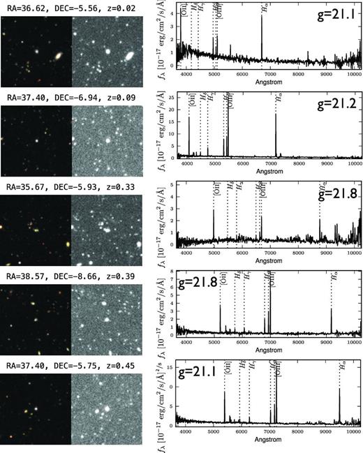
ugr-selected ELGs at z < 0.5. The spectra are represented in fλ convention. The coloured image on the left is courtesy of CFHT cut-out service. The black and white image in the centre is the g band. The observed object is the one in the centre of the images.

ugr-selected ELGs at 0.5 < z < 1.0. The spectra are represented in fλ convention. The coloured image on the left is courtesy of CFHT cut-out service. The black and white image in the centre is the g band. The observed object is the one in the centre of the images.
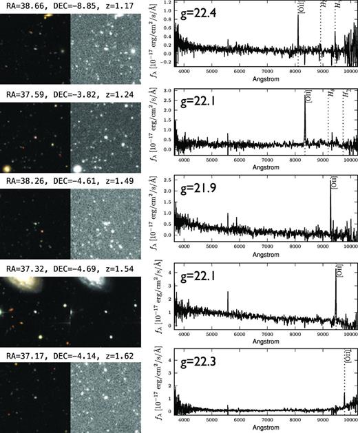
ugr-selected ELGs at 1.0 < z < 1.6. The spectra are represented in fλ convention. The coloured image on the left is courtesy of CFHT cut-out service. The black and white image in the centre is the g band. The observed object is the one in the centre of the images.

ugr-selected quasars at 1.0 < z < 2.3. The spectra are represented in fλ convention. The coloured image on the left is courtesy of CFHT cut-out service. The black and white image in the centre is the g band. The observed object is the one in the centre of the images.
