A fully covariant mean-field dynamo closure for numerical 3 + 1 resistive GRMHD

Bucciantini, N.; Del Zanna, L.

doi:10.1093/mnras/sts005

Abstract

The powerful high-energy phenomena typically encountered in astrophysics invariably involve physical engines, like neutron stars and black hole accretion discs, characterized by a combination of highly magnetized plasmas, strong gravitational fields and relativistic motions. In recent years, numerical schemes for general relativistic magnetohydrodynamics (GRMHD) have been developed to model the multidimensional dynamics of such systems, including the possibility of evolving space–time. Such schemes have been also extended beyond the ideal limit including the effects of resistivity, in an attempt to model dissipative physical processes acting on small scales (subgrid effects) over the global dynamics. Along the same lines, the magnetic field could be amplified by the presence of turbulent dynamo processes, as often invoked to explain the high values of magnetization required in accretion discs and neutron stars. Here we present, for the first time, a further extension to include the possibility of a mean-field dynamo action within the framework of numerical 3 + 1 (resistive) GRMHD. A fully covariant dynamo closure is proposed, in analogy with the classical theory, assuming a simple α-effect in the comoving frame. Its implementation into a finite-difference scheme for GRMHD in dynamical space–times (the x-echo code by Bucciantini & Del Zanna) is described, and a set of numerical test is presented and compared with analytical solutions wherever possible.

gravitation, magnetic fields, MHD, methods: numerical, dynamo, relativis-tic processes

1 INTRODUCTION

A strong magnetic field plays a crucial role in many high-energy astrophysical systems. It is believed to be the key element in the context of gamma-ray bursts (GRBs; Duncan & Thompson 1992; Thompson 1994; Meszaros & Rees 1997; Lee, Wijers & Brown 2000; Lyutikov & Blackman 2001; Vlahakis & Königl 2001; van Putten & Levinson 2003; Lyutikov 2006a; Komissarov & Barkov 2007; Metzger, Thompson & Quataert 2007; Uzdensky &MacFadyen 2007a,b; Barkov & Komissarov 2008; Bucciantini et al. 2008, 2009; Lyons et al. 2010; Metzger et al. 2011; Rezzolla et al. 2011), active galactic nucleus (AGN) jets (Blandford & Znajek 1977; Blandford & Payne 1982; Belvedere & Molteni 1984; Khanna & Camenzind 1992; Konigl & Kartje 1994; Balbus & Hawley 1998; Tomimatsu 2000; Fendt & Memola 2001; Sauty, Tsinganos & Trussoni 2002; van Putten & Levinson 2003; Duttan & Biermann 2007; Hawley 2008; Penna et al. 2010; Tchekhovskoy, Narayan & McKinney 2011), magnetars (Duncan & Thompson 1992; Thompson & Duncan 1996; Murakami 1999; Lyutikov 2003, 2006b; Braithwaite & Spruit 2006; Kasen & Bildsten 2010; Woosley 2010; Yu 2011), and its dissipation and reconnection to be at the origin of many typical high-energy phenomena (Uzdensky 2011). A large-scale ordered magnetic field is in fact crucial to power many high-energy systems. A strong magnetic field close to the central black hole (BH) in accretion discs is invoked to explain the launching of relativistic jets. The pulsar and magnetar paradigms require a strong dipolar magnetic field in neutron stars (NSs). Magnetic field's stresses provide an efficient way to convert the rotational or accretion energy into bulk flow, and to power relativistic winds.

However, the origin of this strong and ordered magnetic field remains poorly understood. In particular, the environment in which such a magnetic field is supposed to arise is often characterized by turbulence (Zhang, MacFadyen & Wang 2009; Mizuno et al. 2011) and instabilities, ranging from Magneto-Rotational Instability (MRI) in accretion discs (Balbus & Hawley 1998) to kink and Tayler and convection in NSs (Miralles, Pons & Urpin 2000, 2002; Braithwaite & Spruit 2006; Rüdiger et al. 2009). While turbulent small-scale motions can easily amplify a seed field up to equipartition with the turbulent kinetic energy, one expects such a field to be highly tangled. If a large-scale ordered mean field can arise due to small-scale velocity fluctuations is highly debated, and understanding what its configuration and its geometry are, and under what conditions it is realized, is of fundamental importance. It is not unreasonable that during the formation of compact objects like BHs or NSs, any frozen-in large-scale field might be amplified due to advection. However, as an explanation of the required magnetic field, this simply shifts the problem from the object to the progenitor. Moreover, in BHs, NSs and GRBs, a large amount of angular momentum is required in the engine, but any strong and pre-existing magnetic field would rapidly slow down the rotation (Duez et al. 2006; Obergaulinger et al. 2006; Bisnovatyi-Kogan, Moiseenko & Ardelyan 2008; Benson & Babul 2009).

Processes that lead to in situ amplification of large-scale magnetic field, due to the dynamics of the flow, are usually referred to as dynamos (Parker 1955, 1987; Moffatt 1978; Cowling 1981; Zeldovich & Ruzmaikin 1987; Roberts & Soward 1992; Kulsrud et al. 1997; Sato 1999; Brandenburg & Subramanian 2005). There are many kinds of dynamo processes but, essentially, all involve twisting of the magnetic field lines by the flow and reconnection events that allow us to re-arrange irreversibly the field topology. Dynamos usually require a fully 3D flow structure. Cowling's theorem, for example, states that dynamos cannot work for 2D flow patterns.

Of particular interest in astrophysics are dynamo processes due to the presence of small-scale fluctuations in the flow and turbulence. The idea that small-scale velocity and magnetic field fluctuations might be correlated, leading to a large-scale effective electromotive force capable of amplifying and generating a large-scale magnetic field, is at the base of the so-called mean-field dynamo theory (Moffatt 1978; Krause & Raedler 1980; Brandenburg & Dobler 2002; Brandenburg & Subramanian 2005). Mean-field dynamos have been applied to a large variety of astrophysical systems, from the Sun (Parker 2009) to stellar magnetism (Brandenburg & Dobler 2002), from accretion discs (Khanna & Camenzind 1996b; Pariev, Colgate & Finn 2007) to proto-NSs (Bonanno, Rezzolla & Urpin 2003), from the origin of the Galactic field (Shukurov 2002) to that of the cosmological primordial field (Kulsrud & Zweibel 2008), just to cite a few.

The formulation of a mean-field closure of Maxwell's equation in the context of General Relativity (GR) has been done only for two astrophysical cases, to our knowledge: Marklund & Clarkson (2005) have investigated the origin of the cosmic magnetic field during inflation, while Khanna & Camenzind (1996a) and Khanna (1999) have focused on the specific case of discs in the Kerr metric. Both have performed some study in the limiting kinematic case, where the back-reaction of the magnetic field on the plasma is neglected. Khanna (1999) has also not considered the displacement current, which however might become non-negligible near the event horizon of a BH, or for rapidly evolving systems. They show that various new terms can arise in GR which are not present in a flat space–time. There is also a debate if Cowling's anti-dynamo theorem still holds in GR: frame dragging effects can generate currents even for axisymmetric configurations (the gravitomagnetic term) in the absence of turbulence (Khanna & Camenzind 1996a).

The possibility of a stable and reliable mean-field closure for turbulent dynamos is however very important in the context of numerical simulations. Quite often large-scale simulations are required to investigate the dynamics of GRB engines, accretion discs in AGN and magnetosphere–jet coupling. The development of small-scale fluctuations is a property of turbulence that makes its numerical investigation within global models prohibitive if not impossible at the moment. The idea behind a mean-field approach is that the effects of physical processes at scales that cannot be resolved can instead be modelled by an appropriate closure of the equations, so that the problem can become treatable by numerical investigation. However, we want to stress here that, in the mean-field approach, determining what could be realistic values for the parameters that are used in the closure is usually non-trivial, and often requires the use of mesoscale information, and extrapolation of flow properties to small unresolved scales. It rests to be proved that a mean-field approach can achieve full resolution of microscopic physics on the macroscale.

Here we present the first fully covariant mean-field dynamo closure of Maxwell's equations, by extending the covariant Ohm's law widely used in resistive general relativistic magnetohydrodynamics (GRMHD; Lichnerowicz 1967; Anile 1989). The new contribution is due to an α-dynamo term proportional to the large-scale magnetic field as measured in the local comoving frame, in analogy to the classical case. Moreover, having in mind numerical applications, the equations are then cast in the 3 + 1 formalism, leading to a modified evolution equation for the spatial electric field as measured by Eulerian observers. When dynamo effects are negligible, the equation reduces to that already derived for resistive magnetohydrodynamic (MHD) in special relativity (Komissarov 2007; Dumbser & Zanotti 2009; Palenzuela et al. 2009), thus extending it to the more general case of 3 + 1 resistive GRMHD. It is not our intention to discuss here either the validity of mean-field dynamo or its theoretical implication within GRMHD. As already done for the purely resistive case, in the above-cited works, here we mainly focus on the numerical implementation of the proposed closure. Our numerical references are the Eulerian Conservative High-Order (echo) and x-echo codes (Del Zanna et al. 2007; Bucciantini & Del Zanna 2011), and the actual implementation and validation tests of this new dynamo closure will refer to these schemes.

The plan of the paper is as follows. In Section 2, we discuss the mean-field closure for the induction equation, and present our covariant GR extension. Section 3 is devoted to its representation in the 3 + 1 formalism, necessary for numerical modelling, whereas in Section 4 we discuss its actual implementation within the x-echo code for GRMHD. In Section 5 we present a set of simple standard tests done both in the so-called kinematic and in the fully dynamic regime, and compare them with previously published results and with analytic and semi-analytic solutions. Finally, we present our conclusion in Section 6.

In the following, we assume a signature −, +, +, + for the space–time metric and we use Greek letters μ, ν, λ, … (running from 0 to 3) for 4D space–time tensor components, while Latin letters i, j, k, … (running from 1 to 3) will be employed for 3D spatial tensor components, and spatial vectors will be often written using boldface characters. Moreover, we set c = G = M_⊙ = 1 and all | $\sqrt{4\pi }$ | factors will be absorbed in the definition of the electromagnetic fields.

2 THE COVARIANT OHM's LAW AND ITS MEAN-FIELD DYNAMO CLOSURE

Let us now briefly discuss the main idea behind the mean-field dynamo theory (Krause & Raedler 1980). Ohm's law for resistive (classical) MHD reads

\begin{equation} \boldsymbol {E} + \boldsymbol {v}\times \boldsymbol {B} = \eta \,\boldsymbol {J}; \quad \boldsymbol {J}= {\nabla }\times \boldsymbol {B}, \end{equation}

(1)

where | $\boldsymbol {E}$ |⁠, | $\boldsymbol {B}$ |⁠, | $\boldsymbol {v}$ | and | $\boldsymbol {J}$ | are the electric field, the magnetic field, the velocity and the current, respectively, and η is the resistivity or coefficient of (isotropic) magnetic diffusivity. If now one separates the quantities into their large-scale mean values | $\bar{\boldsymbol {E}}$ |⁠, | $\bar{\boldsymbol {v}}$ |⁠, | $\bar{\boldsymbol {B}}$ |⁠, and small-scale fluctuating parts | $\delta \boldsymbol {E}, \delta \boldsymbol {v}, \delta \boldsymbol {B}$ |⁠, a new electromotive force due to turbulent motion appears in Ohm's law

\begin{equation} \skew4\bar{\boldsymbol {E}} + \skew4\bar{\boldsymbol {v}} \times \skew4\bar{\boldsymbol {B}} = - \overline{ \delta \boldsymbol {v}\times \delta \boldsymbol {B}} + \eta \skew4\bar{\boldsymbol {J}}; \quad \skew4\bar{\boldsymbol {J}} = {\nabla }\times \skew4\bar{\boldsymbol {B}}. \end{equation}

(2)

In general, the small-scale fluctuating quantities are correlated and thus their product has a non-vanishing mean. The key assumption is that this mean can be written as a function of the mean quantities and their derivatives, and in the simplest case that it is linear in the value of both the mean magnetic field and its curl. Namely, it is often assumed that

\begin{equation} \overline{ \delta \boldsymbol {v}\times \delta \boldsymbol {B}} = \alpha \skew4\bar{\boldsymbol {B}} - \beta \nabla \times \skew4\bar{\boldsymbol {B}}, \end{equation}

(3)

where the two scalar coefficients are both proportional to the local turbulent correlation time τ_c. In particular,

\begin{equation} \alpha = - \textstyle {\frac{1}{3}}\tau _{\rm c} \, \overline{\delta \boldsymbol {v} \times (\nabla \times \delta \boldsymbol {v})}; \quad \beta = \textstyle {\frac{1}{3}}\tau _{\rm c} \,\overline{\delta \boldsymbol {v}^2}, \end{equation}

(4)

where the α-term is proportional to the kinetic helicity and the β-term is related to a random walk for fluid elements. For a deeper insight on the properties of turbulence and a more exhaustive derivation of the α and β terms the reader is referred, for instance, to Kulsrud (2005). Inclusion of magnetic helicity in the definition of α and a different mean-field dynamo closure allowing for a dynamical definition of the electromotive force due to small-scale turbulent fluctuations may be found in Blackman & Field (2002).

Dropping the bars and referring from now on to just large-scale averaged quantities, the classical form for the dynamo closure is then

\begin{equation} \boldsymbol {E} + \boldsymbol {v}\times \boldsymbol {B} = - \alpha \,\boldsymbol {B} + (\beta + \eta )\,\boldsymbol {J}. \end{equation}

(5)

Note that in general both α and β will be tensors; however, we will focus here on the isotropic case where they can be dealt with as scalars. Their values might depend on fluid quantities like density, temperature or magnetic field strength. Moreover, even the specific physical problem at hand could have an influence, as the resulting asymptotic turbulent state may be strongly affected by the assumed initial conditions. When these coefficients can be treated as constants, the induction equation for classical MHD becomes

\begin{equation} \partial _t\boldsymbol {B} = \nabla \times (\boldsymbol {v}\times \boldsymbol {B}) + \alpha \,\nabla \times \boldsymbol {B} + (\beta + \eta )\,\nabla ^2\boldsymbol {B}, \end{equation}

(6)

and it is now apparent that the presence of the α-term may introduce exponentially growing modes that are known as mean-field dynamo waves, whereas the β-term acts as a sort of turbulent diffusivity or turbulent resistivity, which is often dominant over the kinetic one (in the fast-dynamo case). The β-term can be interpreted as due to turbulent mixing: the convection cells mix up magnetic field lines of different polarities on small scales, and thus reduce the mean field, which is equal to the field averaged over larger scales. In the kinematic regime, α, β (and η) are input parameters, as well as | $\boldsymbol {v}$ |⁠, and only the above equation needs to be solved.

Let us finally summarize the mean-field dynamo treatment within classical MHD by rewriting the classical Ohm's law above as

\begin{equation} \boldsymbol {E}^\prime = \xi \,\boldsymbol {B} + \eta \,\boldsymbol {J}, \end{equation}

(7)

i.e. by replacing | $\boldsymbol {E} + \boldsymbol {v}\times \boldsymbol {B} \rightarrow \boldsymbol {E}^\prime$ |⁠, the electric field in the frame comoving with the fluid, − α → ξ (to avoid conflict with the lapse function in the 3 + 1 standard notation, to be introduced in the next section) and β + η → η, combining magnetic and turbulent diffusivity in a single coefficient. In the remainder of this paragraph, we will propose a fully covariant generalization of equation (7), which is novel in the literature, to our knowledge.

The covariant Maxwell's equations are written in terms of the Faraday (anti-symmetric) tensor | $\boldsymbol {F}^{\mu \nu }$ | and its dual | $\boldsymbol {F}^{* \mu \nu } = \frac{1}{2}\epsilon ^{\mu \nu \lambda \kappa }F_{\lambda \kappa }$ |⁠, where ϵ^μνλκ is the space–time Levi-Civita pseudo-tensor [here we use the convention ( − g)^1/2ϵ⁰¹²³ = −( − g)^−1/2ϵ₀₁₂₃ = 1], as

\begin{equation} \nabla _\mu {\boldsymbol F}^{*\mu \nu }=0, \quad \nabla _\mu {\boldsymbol F}^{\mu \nu }=-I^{\nu }, \end{equation}

(8)

where I^μ is the 4-current. The above quantities may be decomposed in the reference frame comoving with the fluid 4-velocity u^μ as

\begin{eqnarray} \boldsymbol {F}^{\mu \nu } = u^\mu e^\nu - e^\mu u^\nu + \epsilon ^{\mu \nu \lambda \kappa }b_\lambda u_\kappa , \end{eqnarray}

(9)

\begin{equation} \boldsymbol {F}^{*\mu \nu } = u^\mu b^\nu - b^\mu u^\nu - \epsilon ^{\mu \nu \lambda \kappa }e_\lambda u_\kappa , \end{equation}

(10)

and

\begin{equation} I^\mu = q_0 u^\mu + j^\mu , \end{equation}

(11)

where | $e^\mu =\boldsymbol {F}^{\mu \nu }u_\nu$ |⁠, | $b^\mu =\boldsymbol {F}^{*\mu \nu }u_\nu$ |⁠, q₀ = −I^μu_μ and j^μ are, respectively, the electric field, magnetic field, charge density and (conduction) current measured in such a frame (e^μu_μ = b^μu_μ = j^μu_μ = 0).

Ohm's law for (isotropic) resistive GRMHD is usually written as a linear relation between the comoving electric field and current (Lichnerowicz 1967; Anile 1989)

\begin{equation} e^\mu = \eta \, j^\mu , \end{equation}

(12)

and the ideal GRMHD relation of a vanishing comoving electric field e^μ = 0 is recovered by letting η = 0 (an ideal plasma with infinite conductivity), which was the closure employed in Del Zanna et al. (2007) and Bucciantini & Del Zanna (2011). The straightforward extension to include a mean-field α-dynamo effect appears to be

\begin{equation} e^\mu =\xi \, b^\mu + \eta \, j^\mu , \end{equation}

(13)

where a new term proportional to the comoving mean magnetic field b^μ now appears and again only the isotropic case has been considered. Both the coefficients ξ and η serve as a sort of subgrid modelling of the turbulent motions, and turbulent diffusivity is supposed to be in general higher than its kinetic value, as in the classical case. Equation (13) is thus our proposed fully covariant generalization of equation (7), to which it correctly reduces in the comoving frame where | $\boldsymbol {v}=0$ | (see the next section).

We want to stress here that, as in the standard mean-field dynamo theory, there is a large degree of freedom in the choice of the closure relations. It can even be debated if a closure in terms of mean quantities and their derivative can be found at all. The quest for an appropriate closure is only apparently more complex in GR, due to the requirement of general covariance, but practically this seems to support the validity of our simple expression in equation (13). However, we want to stress once again that this can be so straightforward only when the isotropic case is assumed, as done in this work for simplicity. Anisotropic resistive MHD in a Minkowskian space–time was considered by Zanotti & Dumbser (2011). On the other hand, our scalar parameters ξ and η may be both functions of all the other (macroscopic) quantities, and thus evolve dynamically in time with them. For simplicity, however, even if the scheme is built to take into account this most general case, numerical tests will be presented only for constants ξ and η.

3 THE DYNAMO CLOSURE IN 3 + 1 GRMHD

In the 3 + 1 formalism, the line element is usually given as

\begin{equation} \mathrm{d}s^2 = - \alpha ^2\mathrm{d}t^2 +\gamma _{ij}(\mathrm{d}x^i+\beta ^i\mathrm{d}t)(\mathrm{d}x^j+\beta ^j\mathrm{d}t), \end{equation}

(14)

where α is the lapse function, βⁱ is the spatial shift vector, both arbitrary due to gauge invariance in the choice of coordinates and γ_ij is the spatial 3-metric, with determinant γ ( − g = α²γ). In this metric, the unit vector of the Eulerian observer's 4-velocity is

\begin{equation} n_\mu = (-\alpha ,0), \quad n^\mu = (1/\alpha ,-\beta ^i/\alpha ), \end{equation}

(15)

and projection on to the spatial hypersurfaces normal to n^μ is achieved via the 3-metric

\begin{equation} \gamma _{\mu \nu } = g_{\mu \nu } +n_\mu n_\nu . \end{equation}

(16)

Spatial projection for a generic vector V^μ (or tensor) is then ⊥V^μ = γ^μ_νV^ν = V^μ + (V^νn_ν)n^μ, and for a spatial vector ⊥V^μ ≡ V^μ. Such a spatial vector must have a vanishing contravariant temporal component, since V^μn_μ = 0.

If we now decompose the electromagnetic quantities within the 3 + 1 Eulerian framework, in analogy with the previous relation we write

\begin{equation} \boldsymbol {F}^{\mu \nu } = n^\mu E^\nu - E^\mu n^\nu + \epsilon ^{\mu \nu \lambda \kappa }B_\lambda n_\kappa , \end{equation}

(17)

\begin{equation} \boldsymbol {F}^{*\mu \nu } = n^\mu B^\nu - B^\mu n^\nu - \epsilon ^{\mu \nu \lambda \kappa }E_\lambda n_\kappa , \end{equation}

(18)

and

\begin{equation} I^\mu = q n^\mu + J^\mu , \end{equation}

(19)

where | $E^\mu =\boldsymbol {F}^{\mu \nu }n_\nu$ |⁠, | $B^\mu =\boldsymbol {F}^{*\mu \nu }n_\nu$ |⁠, q and J^μ are, respectively, the electric field, magnetic field, charge density and (conduction) current measured in such a frame (E^μn_μ = B^μn_μ = J^μn_μ = 0). The Maxwell's equations take the usual form, plus some extra terms due to the 3 + 1 GR metric

\begin{equation} \!\gamma ^{-1/2}\partial _t (\gamma ^{1/2}\boldsymbol {E}) \! - \! {\nabla }\times (\alpha \boldsymbol {B} - \boldsymbol {\beta }\times \boldsymbol {E}) \! = \! - (\alpha \boldsymbol {J}- q\boldsymbol {\beta }), \end{equation}

(20)

\begin{equation} \gamma ^{-1/2}\partial _t (\gamma ^{1/2} \boldsymbol {B}) \! + \! {\nabla }\times (\alpha \boldsymbol {E} + \boldsymbol {\beta }\times \boldsymbol {B}) \! = \! 0, \end{equation}

(21)

\begin{equation} {\nabla }\cdot \boldsymbol {E} = q, \end{equation}

(22)

\begin{equation} {\nabla }\cdot \boldsymbol {B}= 0, \end{equation}

(23)

and we do not repeat here the momentum–energy conservation equation, the continuity equation for the mass density (an equivalent one holds for the electric charge density q) and Einstein's field equations in the 3 + 1 formalism. Compared to ideal GRMHD, where the electric field is a derived quantity, we must now also consider the evolution and constraint equations for | $\boldsymbol {E}$ |⁠, where the sources q and | $\boldsymbol {J}$ | appear.

Let us now see how to treat the various forms of the generalized Ohm's law. It is first convenient to decompose the quantities related to the frame comoving with the fluid within the 3 + 1 Eulerian split of time and space, namely

\begin{equation} u^\mu = \Gamma n^\mu + \Gamma v^\mu , \end{equation}

(24)

\begin{eqnarray} & e^\mu = \Gamma (\boldsymbol {E}\cdot \boldsymbol {v}) n^\mu + \Gamma (E^\mu + \epsilon ^{\mu \nu \lambda }v_\nu B_\lambda ), \end{eqnarray}

(25)

\begin{equation} b^\mu = \Gamma (\boldsymbol {B}\cdot \boldsymbol {v}) n^\mu + \Gamma \big(B^\mu - \epsilon ^{\mu \nu \lambda }v_\nu E_\lambda \big), \end{equation}

(26)

\begin{equation} j^\mu = (q - q_0\Gamma ) n^\mu + J^\mu -q_0\Gamma v^\mu , \end{equation}

(27)

where Γ = (1 − v²)^−1/2 is the Lorentz factor of the fluid flow, | $q_0=\Gamma (q - \boldsymbol {J}\cdot \boldsymbol {v})$ | and ϵ^μνλ = ϵ^μνλκn_κ is the spatial Levi-Civita pseudo-tensor for which γ^1/2ϵ¹²³ = 1. We now have three possibilities:

Ideal GRMHD (e^μ = 0).
The spatial projection readily provides the usual ideal MHD assumption
\begin{equation} \boldsymbol {E} + \boldsymbol {v}\times \boldsymbol {B}= 0, \end{equation}
(28)
exactly as in the classical limit.
Resistive GRMHD (e^μ = ηj^μ).
The time projection leads to | $\Gamma (\boldsymbol {E}\cdot \boldsymbol {v}) = \eta (q-q_0\Gamma )$ |⁠, which may be used to express q₀ in the spatial component. The result is
\begin{equation} \Gamma [\boldsymbol {E} + \boldsymbol {v}\times \boldsymbol {B} - (\boldsymbol {E}\cdot \boldsymbol {v})\boldsymbol {v}] = \eta (\boldsymbol {J} - q\boldsymbol {v}), \end{equation}
(29)
as already found in previous treatments within special relativistic resistive MHD (Komissarov 2007; Dumbser & Zanotti 2009; Palenzuela et al. 2009); thus, here we extend its validity to 3 + 1 GRMHD. When η = 0, we reduce to the previous ideal MHD case, while for | $|\boldsymbol {v}|\ll 1$ |⁠, | $|\boldsymbol {E}|\sim |\boldsymbol {v}||\boldsymbol {B}|$ | we recover the classical limit of equation (1).
Resistive GRMHD + dynamo (e^μ = ξb^μ + ηj^μ).
The time projection is now
\begin{equation} \Gamma (\boldsymbol {E}\cdot \boldsymbol {v}) = \eta (q-q_0\Gamma ) + \xi \Gamma (\boldsymbol {B}\cdot \boldsymbol {v}), \end{equation}
(30)
which again may be used to express q₀ in the spatial component. Now the result is
\begin{eqnarray} &&\!\!\!\Gamma [\boldsymbol {E} + \boldsymbol {v}\times \boldsymbol {B} - (\boldsymbol {E}\cdot \boldsymbol {v})\boldsymbol {v}] \nonumber\\ &&\quad = \eta (\boldsymbol {J} - q\boldsymbol {v}) + \xi \Gamma [\boldsymbol {B} - \boldsymbol {v}\times \boldsymbol {E} - (\boldsymbol {B}\cdot \boldsymbol {v})\boldsymbol {v}], \end{eqnarray}
(31)
which is a novel closure to our knowledge, reducing to the case of resistive GRMHD when ξ = 0 and to the classical case of equation (7) for small velocities.

It is interesting to note that in all cases, the presence of a curved or even evolving GR metric is not apparent in Maxwell's equations, since α or βⁱ terms do not appear explicitly, whereas γ_ij is just needed to work out scalar and cross products between (spatial) vectors.

While in resistive schemes for classical MHD (see e.g. Landi et al. 2008) q and | $\boldsymbol {E}$ | do not play a role and the system is closed simply by taking | $\boldsymbol {J}={\nabla }\times \boldsymbol {B}$ | in Ampere's law, the presence of Maxwell's displacement current in the relativistic case forces one to use equation (20) to evolve the electric field in time. Only in ideal GRMHD is it still possible to neglect the Maxwell equations for the electric field, since | $\boldsymbol {E}$ | is provided from the ideal Ohm's law (equation 28). In the other cases the two equations for | $\boldsymbol {E}$ | must be evolved or preserved in time, and we need to face the problem of dealing with the unknown sources q and | $\boldsymbol {J}$ |⁠. In the proposed scheme we use Ohm's law to provide an expression for the spatial current density | $\boldsymbol {J}$ |⁠, while the constraint on q is enforced by using the Gauss theorem in equation (22). Note that here we do not evolve the charge density via the corresponding continuity equation (charge conservation law), since we choose to impose directly | $q={\nabla }\cdot \boldsymbol {E}$ |⁠.

In the most general case, including mean-field dynamo effects, the result is

\begin{eqnarray} & \gamma ^{-1/2}\partial _t (\gamma ^{1/2}\boldsymbol {E}) - {\nabla }\times (\alpha \boldsymbol {B} - \boldsymbol {\beta }\times \boldsymbol {E}) + (\alpha \boldsymbol {v}- \boldsymbol {\beta }) q \nonumber \\ &= -\; \alpha \Gamma [\boldsymbol {E} + \boldsymbol {v}\times \boldsymbol {B} - (\boldsymbol {E}\cdot \boldsymbol {v})\boldsymbol {v}] /\eta \nonumber \\ &\quad \;+\; \xi \, \alpha \Gamma [\boldsymbol {B} - \boldsymbol {v}\times \boldsymbol {E} - (\boldsymbol {B}\cdot \boldsymbol {v})\boldsymbol {v}] /\eta . \end{eqnarray}

(32)

When η = 0 we can neglect the time-evolution term and the rest of the left-hand side; therefore, time integration of the electric field is not required; also when ξ = 0 we recover the ideal Ohm's law condition | $\boldsymbol {E} = - \boldsymbol {v}\times \boldsymbol {B}$ |⁠, as expected. When η > 0 problems arise because equation (32) is usually stiff, especially for low values of the resistivity, since the source terms on the right are larger than the time-marching term by a large factor 1/η, and some sort of implicit numerical scheme must be employed for time integration. Note that in this respect, the presence of a dynamo α-term adds no further complexity to the numerical algorithm, and its implementation within an existing resistive code is expected to be straightforward.

4 IMPLEMENTATION IN THE echo CODE

Let us discuss here how the closure relation equation (32) can be solved in a numerical scheme for 3 + 1 GRMHD taking as a reference the echo (Del Zanna et al. 2007) and x-echo (Bucciantini & Del Zanna 2011) codes developed in the ideal regime. Here, we propose a very simple method to integrate the equation implicitly. Considering a first-order discretization of the time derivative, one can write an expression for the electric field at the end of a timestep Δt as a function of other quantities, both at the end (superscript ⁽¹⁾) and at the beginning (superscript ⁽⁰⁾) of the implicit procedure.

Introducing the spatial components instead of the vectorial notation, we have

\begin{eqnarray} E^{i(1)}&=& {\gamma ^{(1)}}^{-1/2} {\gamma ^{(0)}}^{1/2} Q^{i(0)}\nonumber \\ &&-\;\big[\Gamma ^{(1)} E^{i(1)}+\epsilon ^{ijk}\tilde{v}_j^{(1)}B_k^{(1)}- \big(E^{k(1)}\tilde{v}_k^{(1)}\big)\tilde{v}^{i(1)}\big/\Gamma ^{(1)}\big]\big/\tilde{\eta } \nonumber \\ &&+\; \xi \big[\Gamma ^{(1)}B^{i(1)} - \epsilon ^{ijk}\tilde{v}_j^{(1)}E_k^{(1)}- \big(B^{k(1)}\tilde{v}_k^{(1)}\big)\tilde{v}^{i(1)}\big/\Gamma ^{(1)}\big]\big/\tilde{\eta },\nonumber\\ \end{eqnarray}

(33)

where rigorously | $\tilde{\eta }=\tilde{\eta }^{(1)}$ | and ξ = ξ⁽¹⁾, since the two coefficients might be in principle function of other variables like temperature, density or magnetic field. The other assumptions are

\begin{eqnarray} \tilde{v}^i &=& \Gamma v^i,\quad \tilde{v}_i = \Gamma v_i,\quad \Gamma ^2=1+\tilde{v}_i \tilde{v}^i,\nonumber \\ Q^{i}&=& E^{i} +\Delta t \big[ - (\alpha v^i-\beta ^i)q + \epsilon ^{ijk} \partial _j \big(\alpha B_k - \epsilon _{klm}\beta ^l E^m\big) \big],\nonumber \\ q &=& \gamma ^{-1/2} \partial _k (\gamma ^{1/2}E^k), \nonumber \\ 1/\tilde{\eta }&=&\Delta t \,\alpha /\eta . \end{eqnarray}

(34)

If we now solve for Eⁱ, after some lengthy algebra we find

\begin{eqnarray} &&\!\!\! E^i [\Gamma + \tilde{\eta } + \xi ^2(\Gamma ^2 - 1)/(\Gamma + \tilde{\eta })] \nonumber \\ &&\quad = -\; \epsilon ^{ijk}\tilde{v}_j B_k + \tilde{\eta }\big[ Q^i+ \big(Q^k \tilde{v}_k\big)\tilde{v}^i \big]\big/ (1+\tilde{\eta } \Gamma ) \nonumber \\ &&\qquad +\; \xi \big[\Gamma B^i- \tilde{\eta } \big(B^k\tilde{v}_k\big)\tilde{v}^i\big/(1+\tilde{\eta }\Gamma )\big] \nonumber \\ &&\qquad -\; \xi \big[(\Gamma ^2 - 1)B^i-\big(\tilde{v}^k B_k\big)\tilde{v}^i + \,\tilde{\eta }\epsilon ^{ijk}\tilde{v}_j Q_k\big]\big/ (\Gamma + \tilde{\eta }) \nonumber \\ &&\qquad+\; \xi ^2\big[\Gamma \epsilon ^{ijk}\tilde{v}_j B_k\big]\big/ (\Gamma + \tilde{\eta }) \nonumber \\ &&\qquad +\; \xi ^2 \big[ \tilde{\eta } \,\Gamma \big(Q^k\tilde{v}_k\big) + \xi \big(B^k\tilde{v}_k\big)\big]\tilde{v}^i\big/ [(1+ \tilde{\eta }\Gamma )(\Gamma + \tilde{\eta }) ],\nonumber\\ \end{eqnarray}

(35)

where for simplicity we have let γ⁽¹⁾^−1/2γ⁽⁰⁾^1/2Qⁱ⁽⁰⁾ → Qⁱ and dropped all superscripts. When ξ = 0, that is in the purely resistive GRMHD case, many terms cancel out and we are left with the simple relation

\begin{equation} E^i (\Gamma + \tilde{\eta }) = - \epsilon ^{ijk}\tilde{v}_j B_k + \tilde{\eta }\big[ Q^i+ \big(Q^k \tilde{v}_k\big)\tilde{v}^i \big]\big/ (1+\tilde{\eta } \Gamma ), \end{equation}

(36)

which automatically includes the limit for an ideal plasma Eⁱ = −ϵ^ijkv_jB_k when η = 0.

4.1 Primitive variables

Equation (35) provides the electric field at the end of a timestep as a function of other primitive variables like the velocity and the magnetic field. However, numerical schemes for GRMHD usually evolve conserved variables like momentum and energy, and primitive variables are not immediately available at the end of a timestep, but must be derived by inverting a set of non-linear equations. This implies that equation (35) must be solved simultaneously with the inversion from conserved variables to primitive. In analogy to Palenzuela et al. (2009), the derivation of the primitive variables and the electric field is done along the following lines.

Given the conserved variables at the end of a timestep, a guess for the pressure p* is chosen, using the value at the previous timestep.
With this value p* of the pressure kept fixed, a guess for the vⁱ* is chosen, again using the values at the previous timestep.
Eⁱ components are derived according to equation (35). This step is performed only when the solution of an implicit equation is required. In general, the Qⁱ contains all of the explicit terms (see the following subsection on time stepping). Equation (34) provides the value of Qⁱ in the simple case for a first-order implicit solver.
The momentum equations are inverted keeping fixed the value p*, by means of a Newton–Raphson scheme, where the Jacobian is computed numerically, to provide a new guess vⁱ* for the vⁱ components. A new electric field is derived and this loop is iterated until convergence.
The energy equation is finally inverted by means of a Newton–Raphson scheme using the values of the velocity vⁱ* and electric field obtained in the inner cycle, to provide a new guess p* for the pressure. Again the derivative required for the Newton–Raphson scheme is computed numerically, allowing for a general equation of state (EoS).
The overall cycle over the pressure p is repeated until convergence.

This approach has the advantage to allow the use of a general EoS; hence, it is not limited to the ideal gas or polytropic EoS, and in principle can be generalized to other closure relations for Ohm's law. We opted for numerical Jacobians, as opposed to approximations to the true analytical ones (Palenzuela et al. 2009), which might be extremely complex to derive and expensive to compute.

The above implementation is straightforward in the Cowling approximation, where the metric terms are fixed in time, but it can also be easily extended to a dynamical space–time by using, for example, the extended conformally flat condition (XCFC) approach as used in x-echo (Cordero-Carrión et al. 2009; Bucciantini & Del Zanna 2011), given that the equation for the evolution of the metric terms is decoupled from the inversion from conserved to primitive variables. The only problem is actually the treatment of the lapse function, appearing in the definition of | $\tilde{\eta }$ |⁠. While in XCFC the conformal factor and the determinant of the 3-metric γ can be easily computed from the conserved quantities, the lapse α requires the previous knowledge of the primitive variables, including the electric field. This implies that one should in principle solve simultaneously for α and the primitive variables. Given that in general the lapse is a slowly and smoothly varying function of time, we prefer to use for simplicity α⁽⁰⁾ in | $\tilde{\eta }$ |⁠, and we expect this choice to introduce only minor errors.

4.2 Time-stepping and constrained transport

The scope of this work is to present and verify the implementation of a dynamo closure in a numerical scheme for 3 + 1 GRMHD. Our code allows the use of two distinct time-stepping approaches: a simple first–second splitting of the temporal evolution, between the implicit and the explicit part, and a more rigorous second-order Implicit Explicit (IMEX) scheme (Pareschi & Russo 2005; Palenzuela et al. 2009). Let us describe here both of them with reference to a typical system of stiff and non-stiff equations, for the conserved variables | $\boldsymbol {U},\boldsymbol {W}$ |⁠:

\begin{eqnarray} \partial _t \boldsymbol {U} &=& \boldsymbol {F}(\boldsymbol {U,W}),\nonumber \\ \partial _t \boldsymbol {W} &=& \boldsymbol {G}(\boldsymbol {U,W})+\frac{1}{\eta }\boldsymbol {R}(\boldsymbol {U,W}). \end{eqnarray}

(37)

In the simple first–second scheme, the explicit part is solved using a modified Eulerian scheme which is second order in time, while a simple first-order scheme is used to solve the implicit one:

\begin{eqnarray} \boldsymbol {U}^{(1)} &=& \boldsymbol {U}^n + \Delta t \boldsymbol {F}(\boldsymbol {U}^n,\boldsymbol {W}^n)/2,\nonumber \\ \boldsymbol {W}^{(1)} &=& \boldsymbol {W}^n +\Delta t \boldsymbol {G}(\boldsymbol {U}^n,\boldsymbol {W}^n)/2 + \frac{\Delta t }{2\eta }\boldsymbol {R}(\boldsymbol {U}^{(1)},\boldsymbol {W}^{(1)}),\nonumber \\ \boldsymbol {U}^{n+1} &=& \boldsymbol {U}^n + \Delta t \boldsymbol {F}(\boldsymbol {U}^{(1)},\boldsymbol {W}^{(1)})\nonumber \\ \boldsymbol {W}^{n+1} &=& \boldsymbol {W}^n +\Delta t \boldsymbol {G}(\boldsymbol {U}^{(1)},\boldsymbol {W}^{(1)}) + \frac{\Delta t }{\eta }\boldsymbol {R}(\boldsymbol {U}^{n+1},\boldsymbol {W}^{n+1}), \end{eqnarray}

(38)

where the implicit step acts only on the electric field | $\boldsymbol {E}$ |⁠, it is performed during the inversion from conserved to primitive variables (see above), according to the solution provided in the previous section.

This simple scheme has the advantage of being easily implementable, requiring only a modification in the definition of the electric field, within the algorithm that derives the primitive from the conserved variables. Moreover, the algorithm is well behaved in the case η = 0 [it reduces to solving | $ \boldsymbol {R}(\boldsymbol {U,W}) =0$ |], and thus it can also handle the ideal MHD regime.

The second-order IMEX that we have implemented is as follows:

\begin{eqnarray} \boldsymbol {U}^{(1)} &=& \boldsymbol {U}^n,\nonumber \\ \boldsymbol {W}^{(1)} &=& \boldsymbol {W}^n + \frac{\Delta t \mu }{\eta }\boldsymbol {R}(\boldsymbol {U}^{(1)},\boldsymbol {W}^{(1)}),\nonumber \\ \boldsymbol {U}^{(2)} &=& \boldsymbol {U}^n + \Delta t \boldsymbol {F}(\boldsymbol {U}^{(1)},\boldsymbol {W}^{(1)}),\nonumber \\ \boldsymbol {W}^{(2)} &=& \boldsymbol {W}^n + \Delta t \boldsymbol {G}(\boldsymbol {U}^{(1)},\boldsymbol {W}^{(1)}) \nonumber \\ && +\; \frac{\Delta t}{\eta }\big[(1-2\mu ) \boldsymbol {R}(\boldsymbol {U}^{(1)},\boldsymbol {W}^{(1)}) +\mu \boldsymbol {R}(\boldsymbol {U}^{(2)},\boldsymbol {W}^{(2)})\big],\nonumber \\ \boldsymbol {U}^{n+1} &=& \boldsymbol {U}^n + \frac{\Delta t}{2}\big[ \boldsymbol {F}(\boldsymbol {U}^{(1)},\boldsymbol {W}^{(1)})+\boldsymbol {F}(\boldsymbol {U}^{(2)},\boldsymbol {W}^{(2)})\big],\nonumber \\ \boldsymbol {W}^{n+1} &=& \boldsymbol {W}^n + \frac{\Delta t}{2}\big[\boldsymbol {G}(\boldsymbol {U}^{(1)},\boldsymbol {W}^{(1)})+\boldsymbol {G}(\boldsymbol {U}^{(2)},\boldsymbol {W}^{(2)})\big]\nonumber \\ && +\; \frac{\Delta t}{2\eta }\big[\boldsymbol {R}(\boldsymbol {U}^{(1)},\boldsymbol {W}^{(1)})+\boldsymbol {R}(\boldsymbol {U}^{(2)},\boldsymbol {W}^{(2)})\big], \end{eqnarray}

(39)

where | $\mu =1-1/\sqrt{2}$ |⁠.

Again the implicit step acts only on the electric field | $\boldsymbol {E}$ |⁠, and it is performed during the inversion from conserved to primitive variables. Note however that now the Qⁱ are no more given simply by equation (34).

However, in comparison with the previous first and second scheme, this IMEX scheme requires three different steps instead of two, the steps do not have the same functional form, and, because of the last step, it is not well behaved in the case η = 0, and so it cannot be used for ideal MHD problems.

All the test that we present in the following have been repeated both without first and second scheme and with the IMEX scheme. As we will discuss, depending on the problem or the desired accuracy, our proposed first/second scheme might offer an easy alternative to more sophisticated IMEX implementations.

The value of the timestep Δt is chosen in accordance to the Courant–Friedrichs–Lewy (CFL) condition, with typical Courant numbers ranging from 0.1 to 0.5 (smaller values have been adopted in high-resistivity runs to avoid large truncation errors in the solution of the implicit part, due to the smaller diffusive time-scale).

As far as the electromagnetic constraints of equations (22) and (23) are concerned, all previously developed schemes for (special) relativistic resistive MHD (Komissarov 2007; Dumbser & Zanotti 2009; Palenzuela et al. 2009) adopt a divergence-cleaning approach (Munz et al. 2000; Dedner et al. 2002), where an augmented system of equations is introduced (including the charge conservation law), and where the solenoidal constraint on the magnetic field and Gauss's theorem is not enforced but preserved by damping and propagating away any violation arising from numerical truncation errors. Here, instead we choose to use a fully constrained scheme, where the charge q appearing in the equation for | $\boldsymbol {E}$ | is taken directly from equation (22) while the divergence-free condition on | $\boldsymbol {B}$ | is treated with staggered grids via the upwind constrained transport method (Londrillo & Del Zanna 2000; Del Zanna, Bucciantini & Londrillo 2003a; Londrillo & del Zanna 2004). A benefit of this fully constrained approach is that, neglecting dynamo effects (ξ = 0) in the purely resistive case, it is possible to recover the ideal MHD expression simply by setting η = 0 (see equation 35), while all previous schemes recover the ideal regime only as a limit for low resistivity η → 0. However, this also depends on the time-stepping algorithm, as we have discussed previously.

To conclude this section, note that in the resistive case the maximum wavespeed is not limited by the fast magnetosonic mode and may approach the speed of light independently of the value of the magnetic field. The Riemann problem at cell interfaces is thus solved for simplicity using the maximally diffusive (global) Lax–Friedrichs (LF) scheme, where the fastest characteristic speed is set to be equal to the speed of light. The use of such a scheme, as opposed to more accurate Riemann solvers like the Harten-Lax-van Leer (HLL) or Harten-Lax-van Leer-Discontinuities (HLLD) might lead to less satisfactory results in the ideal MHD limit, where sharp discontinuities are allowed to arise. In the resistive case, where smooth profiles are expected, the use of more diffusive algorithms is less problematic, especially in conjunction with high-order reconstruction algorithms, a distinguishing feature of our echo scheme. Again, we leave the implementation of more accurate Riemann solvers as a future upgrade.

5 TEST PROBLEMS

In the following, we present a set of standard tests. The first three are done in the purely resistive regime, for comparison with results previously presented in the literature. Then there are three dynamo problems in the so-called kinematic regime, and finally a fully dynamical problem. All but the last of these tests are done in a flat, stationary metric, since they are aimed at evaluating the implementation of the resistive/dynamo closure, and for a more straightforward comparison with previous results, and with analytical solutions.

5.1 Resistive tests

We present here a set of three resistive tests (ξ = 0) in a stationary Cartesian grid (Minkowskian space–time), to be compared with both analytical and previously published results. In the following, we use a third-order Central Essentially Non-Oscillatory (CENO) spatial reconstruction with Monotonized Center (MC) limiter, our both first-order implicit/second-order explicit temporal evolution scheme and the second-order IMEX scheme. A maximally diffusive global LF Riemann solver is employed for upwinding.

5.1.1 Self-similar current sheet

This problem was first proposed by Komissarov (2007), and it has also been presented by Palenzuela et al. (2009) and Dumbser & Zanotti (2009). It is a truly resistive problem, which allows for the analytical self-similar (in t/x²) solution in the limit of infinite pressure:

\begin{equation} B^y(x,t)=B_0 \ {\rm erf} \bigg (\frac{x}{2\sqrt{\eta t}}\bigg ), \end{equation}

(40)

where erf is the error function.

Despite the evolution being almost purely resistive (in principle, in the limit of infinite pressure only the magnetic field evolves and only the induction equation needs to be solved), the problem is followed in the fully dynamical regime. The initial conditions at t = 1 are ρ = 1, p = 50, Eⁱ = 0, vⁱ = 0, B^x = B^z = 0, B^y = B^y(x, 1), with B₀ = 1, and we have adopted an adiabatic coefficient γ = 4/3. Our computational domain extends in the range x = [ − 1.5, 1.5] and is covered by a uniform grid with 200 cells. The problem is evolved to the final time t = 10. In Fig. 1, we compare our numerical results with equation (40), in the case η = 0.01. Errors and convergence estimates are presented in Section 5.3 together with a comparison between the first/second scheme and the IMEX scheme.

Figure 1.

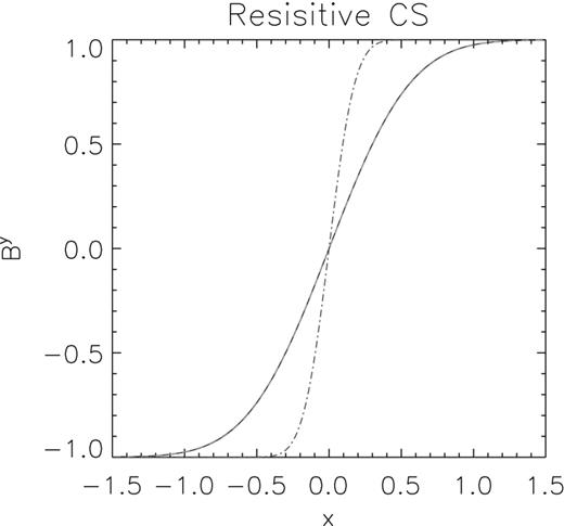
Evolution of the magnetic field in a self-similar current sheet, for η = 0.01. The red dot–dashed line is the initial condition at t = 1. The blue solid line is the numerical solution at t = 10, indistinguishable from the green dashed line representing the exact solution equation (40).

Open in new tab Download slide

5.1.2 Resistive shock tube

This problem was proposed by Dumbser & Zanotti (2009) and differs from the one presented in Palenzuela et al. (2009), which is done in the transverse MHD regime. Shock tubes are excellent tests for monitoring the shock-capturing properties of a numerical scheme. The initial conditions are

\begin{eqnarray} &&\!\!\!(\rho ,p,v^x,v^y,v^z,B^x,B^y,B^z)\nonumber \\ &&\quad =(1.08,0.95,0.4,0.3,0.2,2.0,0.3,0.3)\quad {\rm for}\quad x<0 \nonumber\\ \end{eqnarray}

(41)

and

\begin{eqnarray} &&\!\!\!(\rho ,p,v^x,v^y,v^z,B^x,B^y,B^z)\nonumber \\ &&\quad =(1.0,1.0,-0.45,-0.2,0.2,2.0,-0.7,0.5)\quad {\rm for}\quad x>0,\nonumber\\ \end{eqnarray}

(42)

and the problem is followed to a final time t = 0.55. The initial electric field is set equal to the ideal MHD value Eⁱ = −ϵ^ijkB_jv_k. The computational domain extends in the range x = [ − 0.5, 0.5] and is covered by a uniform grid with 400 cells. The test was repeated with the following values for the resistivity: η = 0, 0.01, 0.1, 1, 1000, where the last value was chosen to be big enough such that the evolution practically corresponds to the zero-conductivity case. The adiabatic coefficient here is γ = 5/3. Results are shown in Fig. 2.

Figure 2.

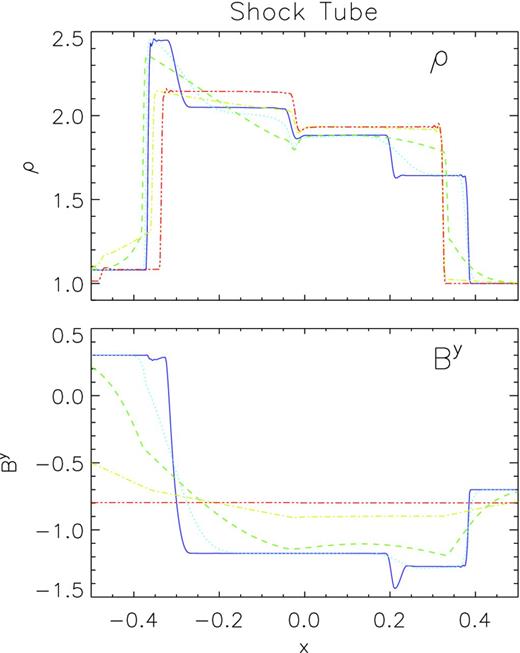
Resistive shock tube problem. The upper panel shows the density and the lower panel shows the y-component of the magnetic field at the final time t = 0.55. The blue solid line is the case η = 0, the dotted cyan line is the case η = 0.01, the green dashed line is the case η = 0.1, the yellow dot–dashed line is the case η = 1, while the red double-dot–dashed line is the case η = 1000.

Open in new tab Download slide

5.1.3 Resistive rotor

This is a fully multidimensional problem. The relativistic ideal MHD version was first proposed by Del Zanna, Bucciantini & Londrillo (2003b), while the resistive version has been presented by Dumbser & Zanotti (2009).

A circular region with radius r = 0.1, uniform density ρ = 10 and rotating with a uniform angular velocity Ω = 8.5 is located within a medium at rest, with a lower density ρ = 1. The pressure p = 1 and the magnetic field (B^x, B^y, B^z) = (1, 0, 0) are uniform in the whole domain. The adiabatic coefficient is γ = 4/3 and the system is followed to a final time t = 0.3. The initial electric field is set equal to the ideal MHD value Eⁱ = −ϵ^ijkB_jv_k. The computational domain is x = [ − 0.5, 0.5], y = [ − 0.5, 0.5], with the rotating region located at the centre, and is covered with a uniform grid of 400 × 400 cells. The problem is solved in the ideal MHD regime η = 0, in the quasi-ideal regime η = 0.001 and in the resistive regime η = 0.1, and the results are shown in Fig. 3. Comparison between the cases η = 0 and 0.001 suggests that, at this resolution, the intrinsic resistivity of the scheme is smaller than η = 0.001. Moreover, the case η = 0, when repeated with a HLL solver (not shown here) does not show any significant improvement with respect to the same case done with LF.

Figure 3.

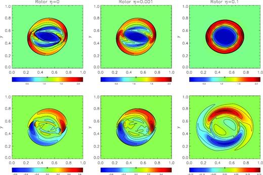
Relativistic rotor. The upper panels show the pressure, while the lower panels show the z-component of the electric field at the final time t = 0.3. Left-hand column: the ideal case η = 0. Central column: quasi-ideal case η = 0.001. Right-hand column: resistive case η = 0.1.

Open in new tab Download slide

5.2 Dynamo tests

Here, we present the tests done using the closure equation (13), leading to the full version in equation (32) of the evolution equation for | $\boldsymbol {E}$ |⁠. The first three are performed in the so-called kinematic regime, where only the induction equation is solved and only the electric and magnetic fields are allowed to change in time. Given the physical nature of mean-field dynamos, related to small-scale turbulence, the kinematic approximation is actually commonly adopted as a suitable approximation. In fact, the magnetic field generated by turbulent dynamo action is often well below equipartition, with respect to the internal energy density, and as such of negligible dynamical consequences. Moreover, kinematic dynamos often allow for simple analytical solutions, whereas the non-linear feedback on the flow can only be dealt with using numerical methods. As for the resistive cases, in all of the following we employ a third-order CENO spatial reconstruction with MC limiter, the maximally diffusive LF solver, and both the usual first-order implicit/second-order explicit and the IMEX time-stepping schemes.

5.2.1 1D steady dynamo

This is a very simple test describing the growth of magnetic field in a stationary medium. It is the dynamo equivalent to the resistive current sheet presented in Section 5.1.1, because it admits an analytical solution (see Appendix A).

We perform a few runs with different resistivity η = 0.05, 0.1, 0.25, different values of the wavenumber k, while ξ = 0.5 is kept fixed. The computational domain x = [ − π, π] is covered with 200 uniformly spaced zones, and the problem is followed to a final time t = 100. Our initial conditions are chosen to correspond to the growing eigenmodes of the problem (see Appendix A):

\begin{eqnarray} B^y&=&0.1\sin {(kx)}, \quad B^x=0, \nonumber \\ B^z&=&-0.1\cos {(kx)}. \end{eqnarray}

(43)

Fig. 4 shows the evolution of the B^y component of the magnetic field, compared with the corresponding analytical expectations, for various values of η and k. It is interesting to note that in the case η = 0.1 and k = 5, the magnetic field is expected to remain unchanged, due to the opposite effects of resistivity and dynamo. Given the nature of the dynamo closure in equation (13), due to round-off and interpolation errors, the evolution of the fastest growing mode however dominates asymptotically. This is what is observed around t = 60: the field starts to grow exponentially, with a growth rate corresponding to the fastest growing mode. The exact time, when this transition happens, depends on roundoff and interpolation errors, and differs for the IMEX scheme.

Figure 4.

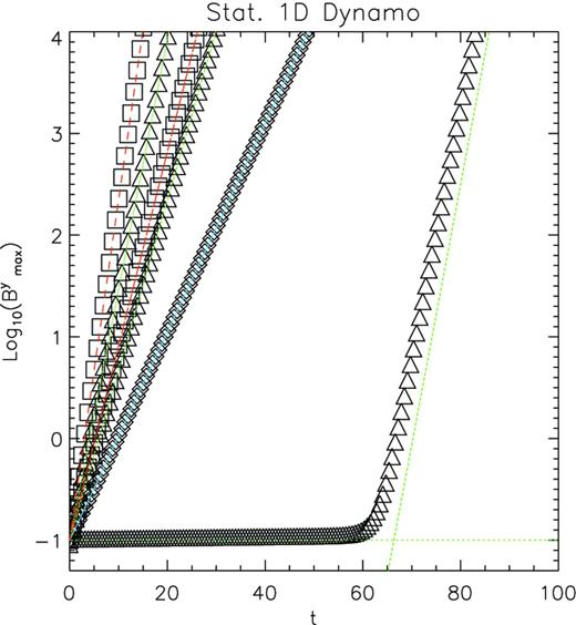
1D steady dynamo. The triangles represent cases with η = 0.1 (and k = 1, 2, 5), the squares η = 0.05 (k = 1, 2) and diamonds η = 0.25 (k = 1). Overplotted is the expected analytical solution with an exponential growth rate Iω: the green dotted lines refer to cases with η = 0.1, corresponding to Iω = 0.385, 0.567, 0.59; the red dashed lines to cases with η = 0.05, corresponding to Iω = 0.44, 0.77; and the solid blue line to η = 0.25, corresponding to Iω = 0.236.

Open in new tab Download slide

In Fig. 5 this property of the dynamo solution is shown for η = 0.05: the initial solution with a wavenumber k = 9 evolves with a slow growth rate until the fastest growing mode, corresponding to k = 5, emerges at t = 12, to dominate the subsequent evolution. Note that, given the exponential nature of the solution, the transition is very sharp. Errors and convergence estimates are presented in Section 5.3 together with a comparison between the first/second scheme and the IMEX scheme.

Figure 5.

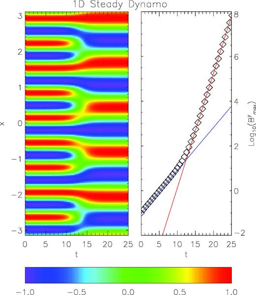
1D steady dynamo, transition to the fastest growing mode. The left-hand panel shows the B^y component of the magnetic field, normalized to its maximum value. The transition from the k = 9 mode to the k = 5 mode happens around t = 12. The right-hand panel shows the evolution of the maximum value of B^y. The solid blue line is the expected growth for a k = 9 mode, the solid red line is the expected growth for the fastest k = 5 mode.

Open in new tab Download slide

5.2.2 Thin shear layer

In this section, we present a 2D shear dynamo problem in the so-called thin-layer approximation, where one of the dimension is assumed to be much smaller than the other, such that higher order variations of all quantities in that direction can be neglected. This is the relativistic equivalent to the 1D problem investigated by Arlt & Rüdiger (1999), where spatial variations of the dynamo coefficient and quenching were also included. The difference between the non-relativistic and the relativistic case is immediately evident. In the former, one just need to add a shear term to the induction equation, proportional to the derivative of the shear velocity along the neglected dimension. However, this is not possible within our relativistic formalism, where the modification due to the dynamo process does not appear in the induction equation, which for us retains the general form given by Maxwell's equations, but instead in the definition of the electric field via the closure of equation (13). For this reason, we adopt the thin-layer approach that allows one to recover the 1D results in the limit of a negligible thickness. This test is representative of typical conditions in accretion discs, in the limit where one models the differential rotation with a shear term in the radial direction and consider modes extending along the vertical direction.

The computational domain is x = [ − π, π], with periodic boundary conditions, and z = [ − δ, δ], with boundary conditions where all quantities are linearly extrapolated. The resistivity is set η = 0.1, while the dynamo term is ξ = 0.2. A shear velocity is imposed to be v^y = 0.9z. The problem is followed to a final time t = 24, corresponding to a dynamo wave period. In Appendix A, the relativistic solution is derived, and we also provide the numerical results for the set of parameters of the present test. Our initial conditions are chosen to correspond to the expected growing eigenmode of the problem

\begin{equation} B^y=0.212\cos (x-0.662), \quad B^x=0, \quad B^z=0.1\sin (x), \end{equation}

(44)

which corresponds to a growth rate ω = −0.238I + 0.261.

The computational domain has 200 equally spaced zones in the x-direction. We have repeated the run varying δ between 0.05 and 0.2, and the number of cells in the z-direction between 5 and 11, and found no appreciable difference in the results. In Fig. 6 we show the evolution and compare the numerical results with the analytical expectations. Both the drifting velocity of the wave and the exponential growth of its amplitude are properly recovered with an accuracy of ∼ 1 per cent. Errors and convergence estimates are presented in Section 5.3 together with a comparison between the first/second scheme and the IMEX scheme, and an estimate of the true growth rate and phase shift.

Figure 6.

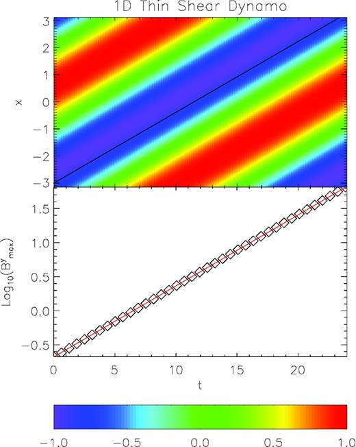
1D thin shear dynamo. The upper panel shows the B^y component of the magnetic field, normalized to its maximum value, as a function of time and space. The solid line represents the analytical phase shift ∝0.261t. The lower panel shows the evolution of the maximum value of B^y. The red solid line is the analytical solution.

Open in new tab Download slide

5.2.3 Kinematic Couette flow

This is a fully 2D dynamo test, on a non-Cartesian grid, corresponding to a Couette flow. We use cylindrical coordinates R, z, with a domain extending in the radial direction in the range R = [0.1, 2], with 100 equally spaced zones, and along the z-direction in the range z = [ − 1, 1], with 100 equally spaced zones. This corresponds to an aspect ratio ∼ 1.

The differential rotation and density (and pressure) stratification are imposed such that the system is in equilibrium, by assuming a polytropic relation p∝ρ^4/3 and requiring that the Bernoulli integral,

\begin{equation} \ln {(h)}+\frac{1}{2}\ln {\big(1-v^\phi v_\phi \big)}-\frac{A}{2}(\Omega -\Omega _0)^2, \end{equation}

(45)

is constant in the domain, where h = 1 + 4p/ρ is the specific enthalpy, v^φ = Ω is the angular velocity, Ω₀ is the angular velocity in R = 0 and the parameter A is an indicator of the amount of differential rotation, since

\begin{equation} v^\phi v_\phi \big/\big(1-v^\phi v_\phi \big)=\Omega A^2 (\Omega -\Omega _0). \end{equation}

(46)

This approach is equivalent to the one used in models of differentially rotating NSs (Komatsu, Eriguchi & Hachisu 1989; Font, Stergioulas & Kokkotas 2000; Bucciantini & Del Zanna 2011). Here, the following values are adopted: Ω₀ = 0.3, ρ(R = 0) = p(R = 0) = 10, A² = 5, which correspond to v^φ(R = 2) = 0.16.

The system is followed to a final time t = 460 corresponding to a dynamo period. Initially a purely toroidal magnetic field is imposed in the computational domain

\begin{eqnarray} B^\phi &=&0.001 \quad {\rm if}\quad \sqrt{(r-1)^2+(Z-0.5)^2} < 0.25, \nonumber \\ B^\phi &=&-0.001 \quad {\rm if}\quad \sqrt{(r-1)^2+(Z+0.5)^2} < 0.25, \end{eqnarray}

(47)

corresponding to two distinct loops, with a zero net magnetic field in the domain. We want to remind here that the shape of the initial magnetic field does not matter, because the system always selects the fastest growing eigenmode of the dynamo equation. The dynamo coefficient is ξ = 0.12, while the resistivity is set to η = 0.03. Periodic boundary conditions are assumed in the z-direction, while a perfect conductor with | $\boldsymbol {E}=0$ | is assumed at the R = 0.1 and 2 boundaries. In Fig. 7 we show the result of the evolution, focusing on the B^φ component. It is evident from the top-right panel that an eigenmode is selected, with a constant drifting speed and an exponential growth.

Figure 7.

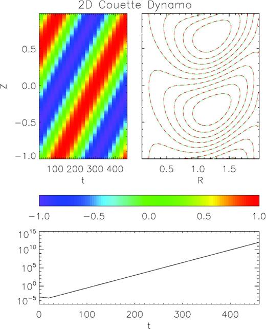
2D Couette flow dynamo. The upper-left panel shows the B^φ component of the magnetic field, in R = 1, normalized to its maximum value, as a function of time. The upper-left panel is a contour plot of B^φ, in the domain at t = 40 (solid cyan lines) and 400 (dashed red lines), after exactly one wavecycle. The lower panel shows the evolution of the maximum value of B^φ.

Open in new tab Download slide

5.2.4 Dynamical NS dynamo in full GRMHD

As a final test we present here the growth of an α² dynamo (no differential rotation or meridional flow) in an NS, in the full dynamical general relativistic regime under the XCFC approximation, as currently employed in the x-echo code. The initial conditions are derived using the xns code by Bucciantini & Del Zanna (2011), to which the reader is referred for a description of parameters characterizing the initial equilibrium configuration. The NS has a central density ρ_c = 1.28 × 10⁻³ (in geometrized units c = G = M_⊙ = 1). The EoS used for the initial settings corresponds to the polytropic relation p = 100ρ²; however, the system is evolved using an ideal gas EoS as done for all NS models in Bucciantini & Del Zanna (2011). The initial magnetic field is purely toroidal and its distribution follows the barotropic law

\begin{equation} \alpha r^2 \sin ^2\theta B^\phi = K_m(\alpha ^2 r^2 \sin ^2\theta \rho h)^m, \end{equation}

(48)

with magnetic parameters K_m = 10⁻⁴ and m = 1. r is the radius and θ is the polar angle.

The 2D simulation is performed in spherical-like coordinates for the conformal flat metric assuming axisymmetry. The computational domain is θ = [ − π, π], with reflecting boundary conditions on the axis, and r = [0, 10], with dipole-like reflecting conditions at the centre and zeroth-order extrapolation at the outer radius. The dipole-like conditions are chosen to allow a dipolar magnetic and electric field where physical quantities like the radial and θ-components of the magnetic field do not vanish in r → 0. The resistivity is set as η = 0.05, while the dynamo coefficient is ξ = 0.1, uniform in the computational domain. The problem is followed to a final time t = 200. The time evolution of the metric is computed once every 100 steps of the MHD part. We want to stress here that these values have been chosen for the sake of having a fast numerical run, and have no physical significance. The scope here is to perform a test of the code in its full dynamical regime, and not to address a particular physical problem in realistic conditions.

In Fig. 8 we show the result of the evolution. The upper panel shows the magnetic configuration that is obtained at the end of the run. The lower panel shows the growth of the maximum value of the poloidal magnetic field during the evolution. Having adopted a uniform ξ term, spurious dynamo action is also present in the atmosphere surrounding the NS. As a consequence a magnetic field develops and grows in the atmosphere too, despite it being completely unmagnetized at the beginning. Again, this is just due to the unphysical choice of a uniform dynamo term. In the figure, for the sake of clarity, we plot the poloidal field just inside the star. It is interesting to note that the growth rapidly approaches an exponential behaviour, but that the slope (the growth rate) changes at around t = 140. This corresponds to the transition to a shorter wavelength. In particular, at the beginning the mode that is excited and grows corresponds to a radial wavelength of the order of twice the stellar radius (given the initial conditions on B^φ). At t = 140 an eigenmode with a shorter radial wavelength of the order of the stellar radius emerges, corresponding to a faster growing mode.

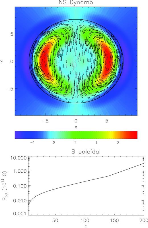
$Dynamical NS dynamo. The upper-panel shows the poloidal magnetic field lines. Colours represent the value of the Bφ component of the magnetic field in units 1015 G. The thick solid line represents the surface of the NS. The lower panel shows the evolution of the maximum value of poloidal magnetic field $\sqrt{B^rB_r+B^{\theta }B_{\theta }}$ .$

Figure 8.

Dynamical NS dynamo. The upper-panel shows the poloidal magnetic field lines. Colours represent the value of the B^φ component of the magnetic field in units 10¹⁵ G. The thick solid line represents the surface of the NS. The lower panel shows the evolution of the maximum value of poloidal magnetic field | $\sqrt{B^rB_r+B^{\theta }B_{\theta }}$ |⁠.

Open in new tab Download slide

5.3 Convergence and comparison between the first/second and IMEX schemes

In this section, we discuss the convergence properties of our scheme and compare the different time-stepping approaches. Despite the simplicity of our first/second scheme, we do expect that, depending on the problem, its accuracy might be closer to first order, as opposed to the IMEX which should preserve second-order accuracy in all cases. We want to stress here that the IMEX scheme we have implemented only acts on the solution of the MHD equations, and it is not integrated with the metric solver. However, in the choice of the XCFC approach, we already assumed that the metric should be slowly varying in time with respect to the plasma. In this case, we do expect that the order of the scheme should not be affected by the metric solver.

We want to point out here that in order to evaluate the convergence of an algorithm, one needs a test problem with a smooth flow structure at all times including the initial conditions, and well-posed boundary conditions that preserve the overall accuracy. If a reference solution, either an analytical solution or a high-resolution run (such that numerical resistivity is smaller than the physical resistivity) for comparison is not available, one can compute the order of convergence using relative errors at different resolutions. In ideal relativistic MHD such a test was designed by Del Zanna et al. (2003b), using a large amplitude, circularly polarized Alfvén wave.

In resistive relativistic MHD no such test has been presented yet. The current sheet problem of Section 5.1.1, admits an exact solution only in the limiting case of infinite pressure. For the value of the pressure that we have used, in line with the previous existing literature, dynamical effects are present, and they dominate the deviations with respect to the solution of equation (40). However, being a 1D problem, it is possible to use a high-resolution run as a reference solution. In Fig. 9, we show the relative error on one component of the magnetic field:

\begin{equation} L_1[B^y(t=\tilde{t})]=\frac{1}{N}\sum _{i=1}^N\frac{\big\Vert B^y(t=\tilde{t})-B^y_{\rm ref}(t=\tilde{t}) \big\Vert }{{\rm max}[B^y (t=\tilde{t})]}, \end{equation}

(49)

where the sum is calculated over the value of the quantity in each of the N cells of the computational domain, and the reference solution at time | $\tilde{t}$ | is obtained interpolating a high-resolution run with 1600 grid points. It is interesting to note that in this test problem the IMEX and our first/second time-stepping algorithm have similar performances, even if the IMEX has a smaller absolute error. This is because the solution is slowly evolving in time and the displacement current is small compared to the conduction current, which is due to spatial gradients of the magnetic field. For this reason, the overall order of the algorithm is dominated by the order of the explicit part of the solver. Moreover, the order seems to be somewhat in between 2 and 3, as expected from the fact that we use a third-order CENO spatial reconstruction.

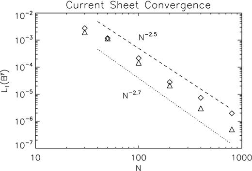
$Convergence test for the resistive current sheet problem. Relative L1 errors on By at $\tilde{t}=10$ , with respect to a high-resolution run with 1600 grid points, in logarithmic scale, as function of the number of grid points. The diamonds represent the first/second scheme and the triangles the IMEX scheme. The dashed and dotted lines represent scaling, respectively, as − 2.5 and − 2.7.$

Figure 9.

Convergence test for the resistive current sheet problem. Relative L₁ errors on B^y at | $\tilde{t}=10$ |⁠, with respect to a high-resolution run with 1600 grid points, in logarithmic scale, as function of the number of grid points. The diamonds represent the first/second scheme and the triangles the IMEX scheme. The dashed and dotted lines represent scaling, respectively, as − 2.5 and − 2.7.

Open in new tab Download slide

For the relativistic dynamo closure, as opposed to the resistive case, the 1D steady dynamos admit analytical solutions. The other multidimensional tests we have presented lack a correct analytical solution and, being multidimensional, it is computationally prohibitive to run a high-resolution reference case; however, as we will show we can use relative errors at different resolutions. In Fig. 10 we show the relative error on one component of the magnetic field, defined as in equation (49) for the 1D steady dynamo with k = 1, η = 0.1, ξ = 0.25. These values have been selected in order for the mode with k = 1 to be the fastest growing mode. 1D steady dynamos are rapidly evolving in time, and with small spatial gradients. The displacement current dominates over the conduction current. The IMEX scheme performs as previously, with an order which is again between 2 and 3 for the same reason as before. The first/second scheme instead reduces to first order as expected.

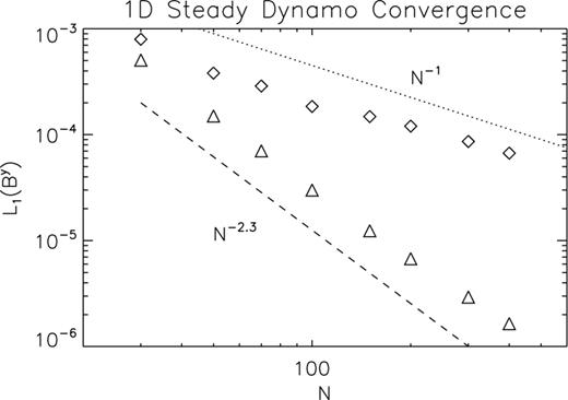
$Convergence test for the 1D steady dynamo problem, with k = 1, η = 0.1 and ξ = 0.25. Relative L1 errors on By at $\tilde{t}=20$ , with respect to the analytical solution, in logarithmic scale, as a function of the number of grid points (per mode wavelength). The diamonds represent the first/second scheme and the triangles the IMEX scheme. The dashed and dotted lines represent scaling, respectively, as − 2.3 and − 1.$

Figure 10.

Convergence test for the 1D steady dynamo problem, with k = 1, η = 0.1 and ξ = 0.25. Relative L₁ errors on B^y at | $\tilde{t}=20$ |⁠, with respect to the analytical solution, in logarithmic scale, as a function of the number of grid points (per mode wavelength). The diamonds represent the first/second scheme and the triangles the IMEX scheme. The dashed and dotted lines represent scaling, respectively, as − 2.3 and − 1.

Open in new tab Download slide

We have also attempted to estimate convergence of the solution and the order of accuracy of our algorithm for the thin shear layer dynamo (Section 5.2.2). We do not have an analytic solution available to use as a reference solution, and it is computationally prohibitive to run a high-resolution case, so we proceed comparing errors in runs of different resolutions. Moreover, we do have an analytic approximated solution and we have an expectation for the functional form of the eigenmode. In particular, we expect the various quantities to evolve as e^−Iωt. So if we assume that the unknown true solution changes in time according to this exponential growth, and that the error of our numerical solutions scales with the number of grid points N as N^−p, we can fit simultaneously for the growth rate, phase shift and accuracy of the scheme. The result is shown in Fig. 11. This is equivalent to estimate the order of accuracy by comparing relative errors. We find that for both the IMEX scheme and our first/second scheme, the best-fitting estimate for ω is ω = −I(0.2383 ± 0.0001) + (0.2626 ± 0.0005), to be compared with the expectation of the approximated analytical solution ω = −0.238I + 0.261. The best fit for the order gives p = 2 ± 0.1 for the IMEX and p = 1.5 ± 0.1 for the first/second scheme. We want to remember here that we use extrapolation for the boundary conditions in the z-direction, and the accuracy of the solution also depends on the boundary conditions that are used.

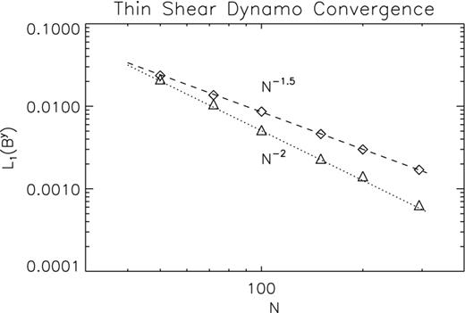
$Convergence fit for the thin shear layer dynamo problem. Relative L1 errors on By at $\tilde{t}=24$ , with respect to the best-fitting reference solution, in logarithmic scale, as function of the number of grid points (per mode wavelength) in the x-direction. The diamonds are for the first/second scheme and the triangles for the IMEX scheme. The dashed and dotted lines represent scaling, respectively, as − 2 and − 1.5.$

Figure 11.

Convergence fit for the thin shear layer dynamo problem. Relative L₁ errors on B^y at | $\tilde{t}=24$ |⁠, with respect to the best-fitting reference solution, in logarithmic scale, as function of the number of grid points (per mode wavelength) in the x-direction. The diamonds are for the first/second scheme and the triangles for the IMEX scheme. The dashed and dotted lines represent scaling, respectively, as − 2 and − 1.5.

Open in new tab Download slide

In all of our tests, we have verified that, at the resolution at which they were performed, the relative errors of the first/second scheme are of the order of a few 10⁻³. Unless one requires higher accuracy, or if the problem involves slowly varying solutions with strong spatial gradients, or for discontinuous solutions, given its easy implementation, we deem this approach satisfactory. The IMEX scheme in general shows better convergence already at 25 points per wavelength of the eigenmode, and should be the algorithm of choice for more demanding cases.

6 CONCLUSION

In this paper, we have presented a fully covariant mean-field α-dynamo closure of the resistive relativistic MHD equations, and shown how it can be implemented within a code for numerical 3 + 1 GRMHD. In particular, we have upgraded the echo code for GRMHD, in its version for dynamical space–times (Bucciantini & Del Zanna 2011). The x-echo scheme employs a fully constrained method for Einstein's equations based on the XCFC, but this particular choice poses no constraint on the applicability of our dynamo closure, which is unchanged in the Cowling approximation (a static GR metric) as well as in other formulations of the Einstein equations. We have shown that our implementation of a dynamo effect is straightforward for any numerical scheme that has already been extended to include resistivity, since the novel generalized Ohm's law is very similar to that for resistive GRMHD and does not pose any additional numerical difficulty. This is true in the simple case proposed here, where an isotropic resistivity and an isotropic α-dynamo term (thus simple proportionality between the electric and magnetic fields in the comoving frame) have been considered. Far more complex closures have been developed for non-relativistic MHD; however, it is not obvious if and how fully covariant equivalent formulations could be found at all. We stress again that determining realistic values for the parameters that are used in the closure, or even finding an appropriate closure, is usually non-trivial, and often requires the use of mesoscale information, and extrapolation of flow properties to small unresolved scales. It rests to be proved that a mean-field approach can achieve full resolution of microscopic physics on the macroscale.

This is the first numerical implementation of a fully covariant dynamo closure for relativistic MHD in the general dynamical regime. Instead of starting with the simpler Minkowskian case, we have directly proposed and applied our model to full GRMHD, exploiting the 3 + 1 formalism, in both static and evolving space–times. We have adopted a fully constrained strategy, to retain the general philosophy of the echo and x-echo schemes. The charge density is derived from Gauss theorem, and it is not evolved as an independent quantity like in previous formulations (no appreciable differences are observed in the numerical tests available in the literature). The solenoidal condition on the magnetic field is preserved to machine accuracy using the upwind constrained transport method on a staggered grid. Stiff terms due to small resistivity in the evolution equation for the (spatial) electric field have been treated both with a simple implicit time-stepping procedure, which allows us, contrary to previous works, to obtain the ideal case of a perfectly conducting plasma simply by setting the resistivity coefficient to zero, and not just as a limit for small resistivity, and with a more roboust IMEX scheme. We have shown that depending on the problem, and in particular on the relative importance of spatial versus temporal gradients, a simple first-order implicit scheme can give satisfactory results, while the IMEX scheme tends to give more reliable performances independently of them.

We have presented a set of standard tests, easily implementable and, where possible, we have compared the numerical results with the analytical expectations, confirming the robustness of the implementation. The majority of the tests have been performed in the so-called kinematic regime. This choice has a physical motivation: mean-field dynamo action arises from small-scale motions that are almost always strongly subsonic. Their kinetic energy is negligible with respect to the internal or gravitational energy of the system. Dynamo action is supposed to be quenched once the strength of the magnetic field reaches equipartition with the kinetic energy of the turbulent motions. As such, one expects that dynamo amplified magnetic fields cannot reach values high enough to affect the global dynamics. However, to verify the stability and robustness of the implementation in a more demanding regime, which must be fully dynamic and closer to a physical application, we have also presented a full dynamical case applied to an NS in GRMHD with a time-dependent metric.

Our results show that it is possible to implement within codes for numerical relativity, a closure that in principle can allow one to model effects arising from dynamics at small scales, that would be prohibitive to follow in global simulations. The general idea of subgridding modelling effects has been widely developed in the context of classical fluid dynamics, but is still in its infancy in the field of numerical relativity. There are several outstanding problems of relativistic fluid dynamics, ranging from the origin of relativistic engines, to their characterization to the dissipative evolution of their magnetic fields, that involve extensive dynamical ranges in space and time. The development of a clever subgridding approach offers an interesting possibility to investigate and model physical processes that otherwise would require a resolution that would be computationally prohibitive. This might lead to a different approach and to a rapid advancement in the field.

We plan to apply our code for dynamo in GRMHD to both accreting discs around BHs and in proto-NSs. These two different environments are fundamentally related to the more promising engines for GRBs, and might have important implications for the general modelling of core-collapse supernovae. Strong magnetic fields have also been invoked for short GRBs, which are commonly considered to be a possible electromagnetic counterpart of binary mergers. Indeed, much of the MHD modelling done until now has focused on the large-scale properties, but it has been shown that the expected magnetic configurations can be highly unstable, and a turbulent cascade is expected. Understanding, if and under what conditions a mean-field dynamo can operate, what is its efficiency, and the geometry and topology of the resulting field, might help to put stronger constraints on to the environment within which they are supposed to operate.

The authors wish to thank A. Bonanno, O. Zanotti, C. Palenzuela and A. Bandenburg for fruitful discussions on issues relating to dynamos, numerical relativity and the solution of the implicit stiff equations. We thank the referee for his fruitful suggestions and comments.

REFERENCES

Anile

A. M.

Anile

A. M.

,

Relativistic Fluids and Magneto-Fluids: With Applications in Astrophysics and Plasma Physics.

,

1989

Cambridge and New York

Cambridge University Press

Google Scholar

Google Preview

OpenURL Placeholder Text

WorldCat

Arlt

R.

Rüdiger

G.

,

A&A

,

1999

, vol.

349

pg.

334

Balbus

S. A.

Hawley

J. F.

,

Rev. Mod. Phys.

,

1998

, vol.

70

pg.

1

Crossref

Search ADS

Barkov

M. V.

Komissarov

S. S.

,

MNRAS

,

2008

, vol.

385

pg.

L28

Crossref

Search ADS

Belvedere

G.

Molteni

D.

,

Phys. Scr.

,

1984

, vol.

7

pg.

163

Crossref

Search ADS

Benson

A. J.

Babul

A.

,

MNRAS

,

2009

, vol.

397

pg.

1302

Crossref

Search ADS

Bisnovatyi-Kogan

G. S.

Moiseenko

S. G.

Ardelyan

N. V.

,

Astron. Rep.

,

2008

, vol.

52

pg.

997

Crossref

Search ADS

Blackman

E. G.

Field

G. B.

,

Phys. Rev. Lett.

,

2002

, vol.

89

pg.

265007

Crossref

Search ADS

PubMed

Blandford

R. D.

Payne

D. G.

,

MNRAS

,

1982

, vol.

199

pg.

883

Crossref

Search ADS

Blandford

R. D.

Znajek

R. L.

,

MNRAS

,

1977

, vol.

179

pg.

433

Crossref

Search ADS

Bonanno

A.

Rezzolla

L.

Urpin

V.

,

A&A

,

2003

, vol.

410

pg.

L33

Crossref

Search ADS

Braithwaite

J.

Spruit

H. C.

,

A&A

,

2006

, vol.

450

pg.

1097

Crossref

Search ADS

Brandenburg

A.

Dobler

W.

,

Astron. Nachr.

,

2002

, vol.

323

pg.

411

Crossref

Search ADS

Brandenburg

A.

Subramanian

K.

,

Phys. Rep.

,

2005

, vol.

417

pg.

1

Crossref

Search ADS

Bucciantini

N.

Del Zanna

L.

,

A&A

,

2011

, vol.

528

pg.

A101

Crossref

Search ADS

Bucciantini

N.

Quataert

E.

Arons

J.

Metzger

B. D.

Thompson

T. A.

,

MNRAS

,

2008

, vol.

383

pg.

L25

Crossref

Search ADS

Bucciantini

N.

Quataert

E.

Metzger

B. D.

Thompson

T. A.

Arons

J.

Del Zanna

L.

,

MNRAS

,

2009

, vol.

396

pg.

2038

Crossref

Search ADS

Cordero-Carrión

I.

Cerdá-Durán

P.

Dimmelmeier

H.

Jaramillo

J. L.

Novak

J.

Gourgoulhon

E.

,

Phys. Rev. D

,

2009

, vol.

79

pg.

024017

Crossref

Search ADS

Cowling

T. G.

,

ARA&A

,

1981

, vol.

19

pg.

115

Crossref

Search ADS

Dedner

A.

Kemm

F.

Kröner

D.

Munz

C.-D.

Schnitzer

T.

Wesenberg

M.

,

J. Comput. Phys.

,

2002

, vol.

175

pg.

645

Crossref

Search ADS

Del Zanna

L.

Bucciantini

N.

Londrillo

P.

,

Mem. Soc. Astron. Ital. Suppl.

,

2003a

, vol.

1

pg.

165

Del Zanna

L.

Bucciantini

N.

Londrillo

P.

,

A&A

,

2003b

, vol.

400

pg.

397

Crossref

Search ADS

Del Zanna

L.

Zanotti

O.

Bucciantini

N.

Londrillo

P.

,

A&A

,

2007

, vol.

473

pg.

11

Crossref

Search ADS

Duez

M. D.

Liu

Y. T.

Shapiro

S. L.

Shibata

M.

Stephens

B. C.

,

Phys. Rev. D

,

2006

, vol.

73

pg.

104015

Crossref

Search ADS

Dumbser

M.

Zanotti

O.

,

J. Comput. Phys.

,

2009

, vol.

228

pg.

6991

Crossref

Search ADS

Duncan

R. C.

Thompson

C.

,

ApJ

,

1992

, vol.

392

pg.

L9

Crossref

Search ADS

Duttan

I.

Biermann

P. L.

Aschenbach

B.

Burwitz

V.

Hasinger

G.

Leibundgut

B.

,

Relativistic Jets in Active Galactic Nuclei: Importance of Magnetic Fields

,

2007

Berlin, Heidelberg

Springer-Verlag

pg.

431

Google Scholar

Google Preview

OpenURL Placeholder Text

WorldCat

Fendt

C.

Memola

E.

,

Ap&SS

,

2001

, vol.

276

pg.

297

Crossref

Search ADS

Font

J. A.

Stergioulas

N.

Kokkotas

K. D.

,

MNRAS

,

2000

, vol.

313

pg.

678

Crossref

Search ADS

Hawley

J.

,

2008

pg.

H3

in APS Meeting Abstracts

Kasen

D.

Bildsten

L.

,

ApJ

,

2010

, vol.

717

pg.

245

Crossref

Search ADS

Khanna

R.

Ferriz-Mas

M. N. A.

,

ASP Conf. Ser. Vol. 178, Stellar Dynamos: Nonlinearity and Chaotic Flows

,

1999

San Francisco

Astron. Soc. Pac.

pg.

57

Google Scholar

Google Preview

OpenURL Placeholder Text

WorldCat

Khanna

R.

Camenzind

M.

,

A&A

,

1992

, vol.

263

pg.

401

Khanna

R.

Camenzind

M.

,

Astrophys. Lett. Commun.

,

1996a

, vol.

34

pg.

53

Khanna

R.

Camenzind

M.

,

A&A

,

1996b

, vol.

307

pg.

665

Komatsu

H.

Eriguchi

Y.

Hachisu

I.

,

MNRAS

,

1989

, vol.

239

pg.

153

Crossref

Search ADS

Komissarov

S. S.

,

MNRAS

,

2007

, vol.

382

pg.

995

Crossref

Search ADS

Komissarov

S. S.

Barkov

M. V.

,

MNRAS

,

2007

, vol.

382

pg.

1029

Crossref

Search ADS

Konigl

A.

Kartje

J. F.

,

ApJ

,

1994

, vol.

434

pg.

446

Crossref

Search ADS

Krause

F.

Raedler

K.-H.

Goodman

L. J.

Love

R. N.

,

Mean-Field Magnetohydrodynamics and Dynamo Theory.

,

1980

Oxford

Pergamon Press

Kulsrud

R. M.

,

Plasma Physics for Astrophysics.

,

2005

Princeton, NJ

Princeton Univ. Press

Google Scholar

Google Preview

OpenURL Placeholder Text

WorldCat

Kulsrud

R. M.

Zweibel

E. G.

,

Rep. Prog. Phys.

,

2008

, vol.

71

pg.

046901

Crossref

Search ADS

Kulsrud

R.

Cowley

S. C.

Gruzinov

A. V.

Sudan

R. N.

,

Phys. Rep.

,

1997

, vol.

283

pg.

213

Crossref

Search ADS

Landi

S.

Londrillo

P.

Velli

M.

Bettarini

L.

,

Phys. Plasmas

,

2008

, vol.

15

pg.

012302

Crossref

Search ADS

Lee

H. K.

Wijers

R. A. M. J.

Brown

G. E.

,

Phys. Rep.

,

2000

, vol.

325

pg.

83

Crossref

Search ADS

Lichnerowicz

A.

Lichnerowicz

A.

,

Relativistic Hydrodynamics and Magnetohydrodynamics.

,

1967

New York

Benjamin

Londrillo

P.

Del Zanna

L.

,

ApJ

,

2000

, vol.

530

pg.

508

Crossref

Search ADS

Londrillo

P.

Del Zanna

L.

,

J. Comput. Phys.

,

2004

, vol.

195

pg.

17

Crossref

Search ADS

Lyons

N.

O'Brien

P. T.

Zhang

B.

Willingale

R.

Troja

E.

Starling

R. L. C.

,

MNRAS

,

2010

, vol.

402

pg.

705

Crossref

Search ADS

Lyutikov

M.

,

MNRAS

,

2003

, vol.

346

pg.

540

Crossref

Search ADS

Lyutikov

M.

,

New J. Phys.

,

2006a

, vol.

8

pg.

119

Crossref

Search ADS

Lyutikov

M.

,

MNRAS

,

2006b

, vol.

367

pg.

1594

Crossref

Search ADS

Lyutikov

M.

Blackman

E. G.

,

MNRAS

,

2001

, vol.

321

pg.

177

Crossref

Search ADS

Marklund

M.

Clarkson

C. A.

,

MNRAS

,

2005

, vol.

358

pg.

892

Crossref

Search ADS

Meszaros

P.

Rees

M. J.

,

ApJ

,

1997

, vol.

476

pg.

232

Crossref

Search ADS

Metzger

B. D.

Thompson

T. A.

Quataert

E.

,

ApJ

,

2007

, vol.

659

pg.

561

Crossref

Search ADS

Metzger

B. D.

Giannios

D.

Thompson

T. A.

Bucciantini

N.

Quataert

E.

,

MNRAS

,

2011

, vol.

413

pg.

2031

Crossref

Search ADS

Miralles

J. A.

Pons

J. A.

Urpin

V. A.

,

ApJ

,

2000

, vol.

543

pg.

1001

Crossref

Search ADS

Miralles

J. A.

Pons

J. A.

Urpin

V. A.

,

ApJ

,

2002

, vol.

574

pg.

356

Crossref

Search ADS

Mizuno

Y.

Pohl

M.

Niemiec

J.

Zhang

B.

Nishikawa

K.-I.

Hardee

P. E.

,

ApJ

,

2011

, vol.

726

pg.

62

Crossref

Search ADS

Moffatt

H. K.

Moffatt

H. K.

,

Magnetic Field Generation in Electrically Conducting Fluids.

,

1978

Cambridge

Cambridge Univ. Press

Google Scholar

Google Preview

OpenURL Placeholder Text

WorldCat

Munz

C.-D.

Omnes

P.

Schneider

R.

Sonnendrcker

E.

Vo

U.

,

J. Comput. Phys.

,

2000

, vol.

161

pg.

484

Crossref

Search ADS

Murakami

T.

,

Astron. Nachr.

,

1999

, vol.

320

pg.

257

Crossref

Search ADS

Obergaulinger

M.

Aloy

M. A.

Dimmelmeier

H.

Müller

E.

,

A&A

,

2006

, vol.

457

pg.

209

Crossref

Search ADS

Palenzuela

C.

Lehner

L.

Reula

O.

Rezzolla

L.

,

MNRAS

,

2009

, vol.

394

pg.

1727

Crossref

Search ADS

Pareschi

L.

Russo

G.

,

J. Sci. Comput.

,

2005

, vol.

25

pg.

129

Pariev

V. I.

Colgate

S. A.

Finn

J. M.

,

ApJ

,

2007

, vol.

658

pg.

129

Crossref

Search ADS

Parker

E. N.

,

ApJ

,

1955

, vol.

122

pg.

293

Crossref

Search ADS

Parker

E. N.

,

Solar Phys.

,

1987

, vol.

110

pg.

11

Crossref

Search ADS

Parker

E. N.

,

Space Sci. Rev.

,

2009

, vol.

144

pg.

15

Crossref

Search ADS

Penna

R. F.

McKinney

J. C.

Narayan

R.

Tchekhovskoy

A.

Shafee

R.

McClintock

J. E.

,

MNRAS

,

2010

, vol.

408

pg.

752

Crossref

Search ADS

Rezzolla

L.

Giacomazzo

B.

Baiotti

L.

Granot

J.

Kouveliotou

C.

Aloy

M. A.

,

ApJ

,

2011

, vol.

732

pg.

L6

Crossref

Search ADS

Roberts

P. H.

Soward

A. M.

,

Annu. Rev. Fluid Mech.

,

1992

, vol.

24

pg.

459

Crossref

Search ADS

Rüdiger

G.

Schultz

M.

Mond

M.

Shalybkov

D. A.

,

Astron. Nachr.

,

2009

, vol.

330

pg.

12

Crossref

Search ADS

Sato

T.

,

J. Plasma Fusion Res.

,

1999

, vol.

75

pg.

7

Crossref

Search ADS

Sauty

C.

Tsinganos

K.

Trussoni

E.

Guthmann

A. W.

Georganopoulos

M.

Marcowith

A.

Manolakou

K.

,

Lecture Notes in Physics, Vol. 589, Relativistic Flows in Astrophysics

,

2002

Berlin

Springer-Verlag

pg.

41

Shukurov

A.

,

Astrophys. & Space Sci.

,

2002

, vol.

281

pg.

285

Crossref

Search ADS

Tchekhovskoy

A.

Narayan

R.

McKinney

J. C.

,

MNRAS

,

2011

, vol.

418

pg.

L79

Crossref

Search ADS

Thompson

C.

,

MNRAS

,

1994

, vol.

270

pg.

480

Crossref

Search ADS

Thompson

C.

Duncan

R. C.

,

ApJ

,

1996

, vol.

473

pg.

322

Crossref

Search ADS

Tomimatsu

A.

,

ApJ

,

2000

, vol.

528

pg.

972

Crossref

Search ADS

Uzdensky

D. A.

,

Space Sci. Rev.

,

2011

, vol.

160

pg.

45

Crossref

Search ADS

Uzdensky

D. A.

MacFadyen

A. I.

,

Phys. Plasmas

,

2007a

, vol.

14

pg.

056506

Crossref

Search ADS

Uzdensky

D. A.

MacFadyen

A. I.

,

ApJ

,

2007b

, vol.

669

pg.

546

Crossref

Search ADS

van Putten

M. H. P. M.

Levinson

A.

,

ApJ

,

2003

, vol.

584

pg.

937

Crossref

Search ADS

Vlahakis

N.

Königl

A.

,

ApJ

,

2001

, vol.

563

pg.

L129

Crossref

Search ADS

Woosley

S. E.

,

ApJ

,

2010

, vol.

719

pg.

L204

Crossref

Search ADS

Yu

C.

,

ApJ

,

2011

, vol.

738

pg.

75

Crossref

Search ADS

Zanotti

O.

Dumbser

M.

,

MNRAS

,

2011

, vol.

418

pg.

1004

Crossref

Search ADS

Zeldovich

Y. B.

Ruzmaikin

A. A.

,

Sov. Phy. Usp.

,

1987

, vol.

30

pg.

494

Crossref

Search ADS

Zhang

W.

MacFadyen

A.

Wang

P.

,

ApJ

,

2009

, vol.

692

pg.

L40

Crossref

Search ADS

APPENDIX A: DYNAMO SOLUTION FOR A RELATIVISTIC THIN SHEAR LAYER

We present here an approximated analytical solution for a simple relativistic shear layer (see problems in Sections 5.2.1 and 5.2.2). It is the relativistic generalization of a problem presented by Arlt & Rüdiger (1999). Let us consider a shear layer, with an extension in the z-direction much smaller than in the x-direction, where we assume that all quantities do not depend on y. Within this layer the velocity has the following profile: v^x = v^z = 0, v^y = Sz, where S is the shear parameter, and does not change in time.

We look for solutions of the form f(z)e^{I(ωt − kx)}, where | $I=\sqrt{-1}$ |⁠. Symmetry tells us that the electric and magnetic fields must have the following parities:

\begin{eqnarray} B^x, E^x &\propto& \bigg [\sum _{i=0}^n a_i z^{2i+1}\bigg ] {\rm e}^{I(\omega t - kx)}, \nonumber \\ B^y, B^z, E^y, E^z &\propto& \bigg [\sum _{i=0}^n a_i z^{2i}\bigg ] {\rm e}^{I(\omega t - kx)}, \end{eqnarray}

(A1)

where the coefficients a_i = B^x_i, E^x_i, B^y_i, … , complex numbers, differ for the various quantities. We will look for a solution up to a z² order.

First, the divergence-free condition on the magnetic field implies B^z₁ = IkB^x₁/2. We start from equation (32) and from the induction equation for the magnetic field, which yield

\begin{eqnarray} &\gamma ^{-1/2}\partial _t (\gamma ^{1/2}B^i) = \epsilon ^{ijk}\partial _j \big(\alpha E_k+ \epsilon _{klm}\beta ^lB^m\big). \end{eqnarray}

(A2)

In the special case of a flat metric in Cartesian coordinates we have α = γ = 1 and βⁱ = 0, then

\begin{eqnarray} &&\!\!\! \xi \left(2 S \left(E^z_1 z^2+E^z_0\right)-2 B^x_0\right)+{\rm i} B^x_0 k S z^2\nonumber \\ &&\quad +\; 4 B^y_1 \eta +2 B^z_0 S+2 I \eta E^x_0 \omega +2 E^x_0=0 \end{eqnarray}

(A3)

\begin{eqnarray} &&\!\!\!\xi \left(2 B^z_0+z^2 \big(2 E^x_0 S+I B^x_0 k\big)\right)\nonumber \\ &&\quad -\;2 I \big(z^2 \big(I B^x_0 S+B^y_1 \eta k+\eta E^z_1 \omega -I E^z_1\big) \nonumber \\ &&\quad +\; B^y_0 \eta k+E^z_0 (\eta \Omega -I)\big)=0 \end{eqnarray}

(A4)

\begin{eqnarray} &&\!\!(-2 \xi (S^2 z^2-1) \left(B^y_1 z^2+B^y_0\right)-B^x_0 \eta (k^2 z^2-2)\nonumber \\ &&\quad -\;2 \big(-I B^z_0 \eta k+z^2 \big(-I \eta E^x_0 k S+{\rm i} \eta E^y_1 \omega +2 \eta E^z_1 S\nonumber \\ &&\quad -\; E^y_1 S^2 z^2+E^y_1)+E^y_0 \big(I \eta \omega -S^2 z^2+1)\big)\big)=0 \end{eqnarray}

(A5)

\begin{eqnarray} &\!\!2E^y_1-I B^x_0 \omega =0 \end{eqnarray}

(A6)

\begin{eqnarray} &\!\!\! \big(-I E^x_0 + E^z_0 k + B^y_0 \omega + E^z_1 k z^2 + B^y_1 \omega z^2 \big)=0 \end{eqnarray}

(A7)

\begin{eqnarray} &\!\!\big(2 I E^y_0 k - 2 I B^z_0 \omega + k \big(2 I E^y_1 + B^x_0 \omega \big) z^2\big)=0. \end{eqnarray}

(A8)

If we impose these relations to be satisfied both at the | ${\cal O}(1)$ | and | ${\cal O} (z^2)$ | order we can get a set of four linear equations for the variables B^x₀, B^y_{0, 1}, B^z₀:

\begin{eqnarray} &-&\!\!I B^x_0 \omega + 1/(-I + \eta \omega )^4 \big(4 a^3 B^z_0 \eta S^3 + B^x_0 \eta (-I + \eta \omega )^2 \nonumber \\ &&(2 S^2 + k^2 (1 + I \eta \omega )) + 2 a^2 \eta S^2 \big(B^x_0 (-2 - 2 I \eta \omega ) \nonumber \\ &&+\; k \big(-2 I B^y_0 \eta S + B^z_0 (-I + \eta \omega )\big)\big) + 2 I a (-I + \eta \omega ) \nonumber \\ &&\big(B^y_1 (1 + 2 I \eta \omega + \eta ^2 (4 S^2 - \omega ^2)) + \eta S^2 (2 B^z_0 S \nonumber \\ &&+ B^y_0 (-\eta k^2 - I \omega + \eta \omega ^2)\big)\big)\big)=0 \end{eqnarray}

(A9)

\begin{eqnarray} 1/(-I &+& \eta \omega )^2 \big(-\xi ^2 B^z_0 S - I (-I + \eta \omega ) \big(2 B^y_1 \eta - B^y_0 \eta k^2 \nonumber \\ &&+\; B^z_0 S - I B^y_0 \omega + B^y_0 \eta \omega ^2\big) + \xi (B^x_0 + I B^x_0 \eta \omega \nonumber \\ &&+\;I k \big(B^z_0 + B^y_0 \eta S + I B^z_0 \eta \omega \big)\big)=0 \end{eqnarray}

(A10)

\begin{eqnarray} B^z_0 \omega + \big(I k \big(\xi B^y_0 + \eta \big(B^x_0 + I B^z_0 k\big)\big)\big)\big/(-I + \eta \omega )=0 \end{eqnarray}

(A11)

\begin{eqnarray} &&\!\!\!B^y_1 \omega + 1/(2 (-I + \eta \omega )^3) k \big(-2 I a^3 B^z_0 S^2 - 2 \big(B^y_1 \eta k \hphantom\nonumber \\ &&\quad +\; I B^x_0 S\big) (-I + \eta \omega )^2 - 2 \xi ^2 S \big(B^y_0 \eta k S + B^x_0 (-I + \eta \omega )\big) \nonumber \\ &&\quad +\; a (-I + \eta \omega ) \big(2 S \big(2 B^y_1 \eta + B^z_0 S\big) + B^x_0 k (-I + \eta \omega \big))\big)\big)\nonumber\\ &&\quad =0. \end{eqnarray}

(A12)

Imposing that the determinant of the matrix representative of this system vanishes provides us with a fifth-order equation for ω as a function of k, η, ξ, S which is our dispersion relation.

For example, in the case ξ = 0.2, η = 0.1, k = 1 and S = 0.9 we find a growing mode solution with ω = 0.261 − 0.238I. To this mode it corresponds an eigenvector with |B^y₀|/|B^x₀| = 2.13 and with a phase difference between these two components δφ = 0.66. The non-relativistic case, instead, where displacement currents and charge densities are neglected, and where an exact analytical solution can be found, gives ω = 0.254 − 0.240I.

In the case S = 0, it is possible to find an exact analytical solution for the dispersion relation and the eigenmodes

\begin{eqnarray} I (-\xi k - \eta k^2 - I \omega + \eta \omega ^2)/(-I + \eta \omega )=0, \end{eqnarray}

(A13)

which gives

\begin{eqnarray} \omega = I[1 \pm \sqrt{1 + 4 \eta k (\xi -\eta k)}]/(2 \eta ). \end{eqnarray}

(A14)

Exponentially growing modes are possible only for k < ξ/η. The quantity ξ/ηk is the dynamo number. The fastest growing mode has k = ξ/(2η) and a growth rate | $\omega _{{\rm max}} = (\sqrt{1+\xi ^2} -1)/(2\eta )$ |⁠. The eigenmode corresponding to the growing solution is

\begin{eqnarray} B^y &=& IB^z,\quad B^x=0,\quad E^x=0\nonumber \\ E^y&=&\frac{I(\xi B^y +IB^z\eta k)}{I-\eta \omega }\nonumber \\ E^z&=&\frac{I\xi B^z +B^y\eta k}{I-\eta \omega }. \end{eqnarray}

(A15)

This solution can be compared with the non-relativistic case, where the displacement current is neglected

\begin{eqnarray} \omega &=&Ik(a-\eta k)\nonumber \\ B^y &=& IB^z,\quad B^x=0.\nonumber \\ E^y&=&\xi B^y +IB^z\eta k\nonumber \\ E^z&=&\xi B^z -IB^y\eta k. \end{eqnarray}

(A16)

Download all slides

Month:	Total Views:
January 2017	8
February 2017	3
March 2017	10
April 2017	3
June 2017	22
July 2017	6
August 2017	4
September 2017	1
October 2017	7
November 2017	1
December 2017	11
January 2018	9
February 2018	18
March 2018	22
April 2018	12
May 2018	18
June 2018	9
July 2018	24
August 2018	8
September 2018	24
October 2018	16
November 2018	27
December 2018	24
January 2019	14
February 2019	15
March 2019	15
April 2019	24
May 2019	25
June 2019	14
July 2019	12
August 2019	30
September 2019	7
October 2019	13
November 2019	21
December 2019	13
January 2020	15
February 2020	14
March 2020	13
April 2020	12
May 2020	16
June 2020	11
July 2020	19
August 2020	9
September 2020	9
October 2020	12
November 2020	10
December 2020	9
January 2021	8
February 2021	29
March 2021	28
April 2021	21
May 2021	23
June 2021	8
July 2021	17
August 2021	14
September 2021	16
October 2021	10
November 2021	20
December 2021	13
January 2022	12
February 2022	9
March 2022	16
April 2022	12
May 2022	6
June 2022	15
July 2022	17
August 2022	22
September 2022	17
October 2022	25
November 2022	10
December 2022	14
January 2023	27
February 2023	19
March 2023	25
April 2023	28
May 2023	19
June 2023	9
July 2023	10
August 2023	11
September 2023	14
October 2023	15
November 2023	12
December 2023	17
January 2024	18
February 2024	22
March 2024	27
April 2024	11
May 2024	23
June 2024	26
July 2024	24
August 2024	17
September 2024	12
October 2024	26
November 2024	21
December 2024	31
January 2025	25
February 2025	23
March 2025	30
April 2025	9
May 2025	20

Article Contents

A fully covariant mean-field dynamo closure for numerical 3 + 1 resistive GRMHD

Abstract

1 INTRODUCTION

2 THE COVARIANT OHM's LAW AND ITS MEAN-FIELD DYNAMO CLOSURE

3 THE DYNAMO CLOSURE IN 3 + 1 GRMHD

4 IMPLEMENTATION IN THE echo CODE

4.1 Primitive variables

4.2 Time-stepping and constrained transport

5 TEST PROBLEMS

5.1 Resistive tests

5.1.1 Self-similar current sheet

5.1.2 Resistive shock tube

5.1.3 Resistive rotor

5.2 Dynamo tests

5.2.1 1D steady dynamo

5.2.2 Thin shear layer

5.2.3 Kinematic Couette flow

5.2.4 Dynamical NS dynamo in full GRMHD

5.3 Convergence and comparison between the first/second and IMEX schemes

6 CONCLUSION

REFERENCES

APPENDIX A: DYNAMO SOLUTION FOR A RELATIVISTIC THIN SHEAR LAYER

Citations

Views

Altmetric

Email alerts

Astrophysics Data System

Citing articles via

Latest

Most Read

Most Cited

Article Contents

A fully covariant mean-field dynamo closure for numerical 3 + 1 resistive GRMHD Free

Abstract

1 INTRODUCTION

2 THE COVARIANT OHM's LAW AND ITS MEAN-FIELD DYNAMO CLOSURE

3 THE DYNAMO CLOSURE IN 3 + 1 GRMHD

4 IMPLEMENTATION IN THE echo CODE

4.1 Primitive variables

4.2 Time-stepping and constrained transport

5 TEST PROBLEMS

5.1 Resistive tests

5.1.1 Self-similar current sheet

5.1.2 Resistive shock tube

5.1.3 Resistive rotor

5.2 Dynamo tests

5.2.1 1D steady dynamo

5.2.2 Thin shear layer

5.2.3 Kinematic Couette flow

5.2.4 Dynamical NS dynamo in full GRMHD

5.3 Convergence and comparison between the first/second and IMEX schemes

6 CONCLUSION

REFERENCES

APPENDIX A: DYNAMO SOLUTION FOR A RELATIVISTIC THIN SHEAR LAYER

Citations

Views

Altmetric

Email alerts

Astrophysics Data System

Citing articles via

Latest

Most Read

Most Cited

This Feature Is Available To Subscribers Only

A fully covariant mean-field dynamo closure for numerical 3 + 1 resistive GRMHD