


Abstract
Using Very Large Telescope/Fibre Large Array Multi Element Spectrograph optical integral field unit observations, we present a detailed study of UM 448, a nearby blue compact galaxy (BCG) previously reported to have an anomalously high N/O abundance ratio. New Technology Telescope/Superb-Seeing Imager images reveal a morphology suggestive of a merger of two systems of contrasting colour, whilst our Hα emission maps resolve UM 448 into three separate regions that do not coincide with the stellar continuum peaks. UM 448 exhibits complex emission line profiles, with most lines consisting of a narrow [full width at half-maximum (FWHM) ≲ 100 km s−1], central component, an underlying broad component (FWHM ∼ 150–300 km s−1) and a third, narrow blueshifted component. Radial velocity maps of all three components show signs of solid body rotation across UM 448, with a projected rotation axis that correlates with the continuum morphology of the galaxy. A spatially resolved, chemodynamical analysis, based on the [O iii] λλ4363, 4959, [N ii] λ6584, [S ii] λλ6716, 6731 and [Ne iii] λ3868 line maps, is presented. Whilst the eastern tail of UM 448 has electron temperatures (Te) that are typical of BCGs, we find a region within the main body of the galaxy where the narrow and broad [O iii] λ4363 line components trace temperatures differing by 5000 K and oxygen abundances differing by 0.4 dex. We measure spatially resolved and integrated ionic and elemental abundances for O, N, S and Ne throughout UM 448, and find that they do not agree, possibly due the flux weighting of Te from the integrated spectrum. This has significant implications for abundances derived from long-slit and integrated spectra of star-forming galaxies in the nearby and distant universe. A region of enhanced N/O ratio is indeed found, extended over a ∼0.6 kpc2 region within the main body of the galaxy. Contrary to previous studies, however, we do not find evidence for a large Wolf–Rayet (WR) population, and conclude that WR stars alone cannot be responsible for producing the observed N/O excess. Instead, the location and disturbed morphology of the N-enriched region suggest that interaction-induced inflow of metal-poor gas may be responsible.
1 INTRODUCTION
Observations of blue compact galaxies (BCGs) in the nearby Universe provide a means for studying chemical evolution and star formation (SF) processes in chemically unevolved environments. Their low metallicities make them attractive as analogues to the young ‘building-block’ galaxies thought to exist in the high-z primordial universe (Searle & Sargent 1972). BCGs are thought to have experienced only very low level SF in the past, but are currently undergoing bursts of SF in relatively pristine environments, ranging from 0.02 to 0.5 solar metallicity (Kunth & Östlin 2000). Thus understanding the chemical evolution within BCGs can impact upon our understanding of primordial galaxies and galaxy evolution in general.
The distribution of nitrogen as a function of metallicity in SF galaxies has often been a cause for debate, especially at intermediate metallicities [7.6 ≤ 12+log(O/H) ≤ 8.3]. Within this metallicity range the N/O abundance ratio indicates that nitrogen behaves neither as a primary element (i.e. N/O independent of O/H) nor as a secondary element (i.e. N/O proportional to O/H); instead a large scatter is observed. In particular, several BCGs exist whose N/O abundance ratios are up to three times those expected for their O/H values, as highlighted by e.g. Pustilnik et al. (2004). Several of these galaxies have been the focus of our spectroscopic studies using integral field unit (IFU) observations (James et al. 2009; James, Tsamis & Barlow 2010), aimed at understanding the source of such abundance peculiarities.
James et al. (2009) performed a detailed abundance analysis of the N/O-outlier BCG, Mrk 996, whose X-ray properties have been studied by Georgakakis et al. (2011). Previous long-slit observations of this galaxy (Thuan, Izotov & Lipovetsky 1996; Pustilnik et al. 2004) had shown it to have N/O ratio values at least ∼4 times higher than those of other BCGs of similar metallicity. Using IFU observations, James et al. (2009) performed a spatially resolved multi-component emission line analysis of Mrk 996, which revealed a 20-fold N/O and N/H enrichment factor in the broad component [400–500 km s−1 full width at half-maximum (FWHM)] versus the narrow component line emission. The narrow component gas on the other hand has an N/O ratio which is typical for the galaxy's metallicity. In this respect, Mrk 996 is similar to NGC 5253, a starburst galaxy for which an enhanced N/O ratio has also been isolated to broad component gas (López-Sánchez & Esteban 2010). In Mrk 996, the spatial morphology of the broad line component is highly correlated with Wolf–Rayet (WR) wind-feature emission arising from a population of WNL (‘late’ type, nitrogen-rich) stars, strongly suggesting the enhanced nitrogen to be the result of chemical enrichment by the N-rich winds of WN-type WR stars. This supports the postulate of nitrogen self-enrichment due to WR stars that had been suggested by Walsh & Roy (1987) and Pagel, Terlevich & Melnick (1986) to explain elevated N/O levels.
James et al. (2010) also presented an integral field spectroscopic study of the interacting dwarf galaxy UM 420 for which the long-slit spectroscopic study of Izotov & Thuan (1999) had reported log(N/O) = −1.08. By performing a spatially resolved analysis of its physical and chemical conditions, James et al. (2010) found an average ratio applicable to the whole galaxy of log(N/O) = −1.64, i.e. 3.6 times lower than previous estimates. The Very Large Telescope (VLT) observations of James et al. (2010) did not confirm previous detections of WR spectral features in UM 420, highlighting the difficulties involved in identifying WR stellar populations in distant dwarf galaxies.
In this paper, we present IFU observations of another member of this subset of potentially N/O-anomalous galaxies, UM 448 (UGC 06665 and Mrk 1304). With a reported factor of ∼3 nitrogen excess (Bergvall & Östlin 2002), this galaxy presents an excellent opportunity to further our understanding of peculiar N/O ratios in some BCGs and the mechanisms responsible. UM 448 is a complex system, with a disturbed morphology possibly due to a merger event (Dopita et al. 2002). Thus the need for spatially resolved spectroscopy is two-fold: first in determining the range of physical properties and chemical compositions that are present, and secondly, in spatially relating any chemical anomalies to environmental factors (e.g. WR populations).
UM 448 is a starburst galaxy (Keel & van Soest 1992; Kewley et al. 2001) consisting of various star-forming knots, diffuse Hα emission in the north and an SE tidal extension (Dopita et al. (2002)). Broad He ii λ4686 emission was detected by Masegosa, Moles & del Olmo (1991) and subsequently by Guseva, Izotov & Thuan (2000), who reported an atypical weakness in this line in comparison with other WR-signature lines. As with Mrk 996 and NGC 5253, a WR population may well be the source of N-enhancement within this BCG.
In this paper we present integral field spectroscopy (IFS) observations obtained with the VLT-Fibre Large Array Multi Element Spectrograph (FLAMES) IFU. Crucially, this instrument is sufficiently blue-sensitive to detect the [O ii] λ3727 doublet line, meaning that we are not required to adopt uncertain ionization correction factors (ICFs) to determine oxygen abundances. These data afford us a new spatiokinematic 3D view of UM 448, with the spatial and spectral resolution to undertake a full multivelocity component analysis. We adopt a distance of 75.9 Mpc for UM 448 from the velocity measured here of +5579 ± 5 km s−1 (z = 0.018660 ± 1.6 × 10⁻⁵), with a Hubble constant of H0 = 73.5 km s−1 Mpc−1 (DeBernardis et al. 2008).
2 OBSERVATIONS AND DATA REDUCTION
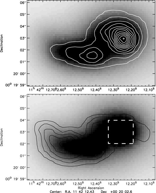
Observations of UM 448 were obtained with the FLAMES (Pasquini et al. 2002) at Kueyen, Telescope Unit 2 of the 8.2-m VLT at ESO’s observatory on Paranal, in service mode on dates specified in Table 1. Observations were made with the Argus IFU, with a field of view (FoV) of 11.5 × 7.3 arcsec2 and a sampling of 0.52 arcsec lens−1. In addition to science fibres, Argus has 15 sky-dedicated fibres that simultaneously observe the sky and that were arranged to surround the IFU FoV at distances of ∼35–58 arcsec. The positioning of the IFU aperture for UM 448 is shown overlaid on Superb-Seeing Imager (SuSI2) images1 in Fig. 1.
![Superb-Seeing Imager [SuSI2, installed on the ESO 3.5-m New Technology Telescope (NTT) at La Silla Observatory, Chile] colour-composite images of UM 448 (red: R band; green: V band; and blue: B band), with the 11.5 × 7.3 arcsec2 FLAMES IFU aperture overlaid. Each image has been scaled to enhance different features within UM 448. The left-hand panel shows two large knots of continuum or ionized gas emission that extend away from the galaxy in a south-westerly direction, outside the IFU FoV. The right-panel shows the two distinct portions of the galaxy, a blue eastern tail and a reddish knot of stellar continuum. SuSI2 images were obtained from the ESO archive, observed as part of programme 078.B-0358(A).](https://oup.silverchair-cdn.com/oup/backfile/Content_public/Journal/mnras/428/1/10.1093/mnras/sts004/2/m_86fig1.jpeg?Expires=1750509854&Signature=EQoVY0DiEdDpWRCka9QpNvi5rPj3zNemF1Qb06NZU~y2OepIVrc6MJ~ErYyFkC1DxYw~HvTXdXaDQTDVWDsau-OuhgqCMuMplLLTgMCRAS7aOlqwNSvrxHfkZBLD54YVsKvK7OrA57LOwnniNSQ12xmsjgjeNGt0DDCFPTCfSj8l6DfoWti-lAu6twATeRrRdrKVrePymqqedGBPX9G4AriniVMleodVrLIgKzLI3S8iNuq-at1rRUT-~kGByEIaWcy~n6SbVdC3W3HXvcb4yATg8QrTaGIEg09bN0ZxEvGP3wbxy2wGrLDzyySig75gjSB91lwtEuAm7h1bJrAosw__&Key-Pair-Id=APKAIE5G5CRDK6RD3PGA)
Superb-Seeing Imager [SuSI2, installed on the ESO 3.5-m New Technology Telescope (NTT) at La Silla Observatory, Chile] colour-composite images of UM 448 (red: R band; green: V band; and blue: B band), with the 11.5 × 7.3 arcsec2 FLAMES IFU aperture overlaid. Each image has been scaled to enhance different features within UM 448. The left-hand panel shows two large knots of continuum or ionized gas emission that extend away from the galaxy in a south-westerly direction, outside the IFU FoV. The right-panel shows the two distinct portions of the galaxy, a blue eastern tail and a reddish knot of stellar continuum. SuSI2 images were obtained from the ESO archive, observed as part of programme 078.B-0358(A).
FLAMES IFU observing log.
| Date | Grism | Wavelength range (Å) | Exp. time (s) | Avg. airmass | FWHM seeing (arcsec) | Standard star |
|---|---|---|---|---|---|---|
| 24/05/2009 | LR1 | 3620–4081 | 3 × 233 | 1.11 | 0.85 | LTT 7379 |
| – | LR2 | 3964–4567 | 3 × 300 | 1.12 | 0.87 | LTT 7379 |
| – | LR3 | 4501–5078 | 3 × 230 | 2.24 | 0.80 | LTT 7379 |
| 18/06/2009 | LR1 | 3620–4081 | 3 × 233 | 1.12 | 0.47 | Feige 110 |
| – | LR2 | 3964–4567 | 3 × 300 | 1.13 | 0.42 | Feige 110 |
| – | LR3 | 4501–5078 | 3 × 230 | 1.16 | 0.50 | Feige 110 |
| 28/07/2009 | LR6 | 6438–7184 | 3 × 400 | 1.75 | 0.47 | EG 21 |
| 26/01/2010 | LR1 | 3620–4081 | 3 × 233 | 1.15 | 0.54 | LTT 4364 |
| – | LR2 | 3964–4567 | 3 × 300 | 1.13 | 0.53 | LTT 4364 |
| – | LR3 | 4501–5078 | 3 × 230 | 1.11 | 0.63 | LTT 4364 |
| 16/03/2010 | LR1 | 3620–4081 | 3 × 233 | 1.10 | 0.57 | LTT 4364 |
| – | LR2 | 3964–4567 | 3 × 300 | 1.11 | 0.50 | LTT 4364 |
| – | LR3 | 4501–5078 | 3 × 230 | 1.12 | 0.56 | LTT 4364 |
| 08/07/2010 | LR6 | 6438–7184 | 8 × 600 | 1.63 | 0.77 | Feige 110 |
| 09/07/2010 | LR1 | 3620–4081 | 3 × 233 | 1.50 | 0.77 | Feige 110 |
| – | LR2 | 3964–4567 | 3 × 300 | 1.60 | 0.72 | Feige 110 |
| – | LR3 | 4501–5078 | 3 × 230 | 1.74 | 0.66 | Feige 110 |
Four different low-resolution (LR) gratings were utilized: LR1 (λλ3620–4081, 24.9 ± 0.3 km s−1 FWHM resolution), LR2 (λλ3964–4567, 24.7 ± 0.1 km s−1), LR3 (λλ4501–5078, 24.6 ± 0.3 km s−1) and LR6 (λλ6438–7184, 21.9 ± 0.4 km s−1). This enabled us to cover all the important emission lines needed for an optical abundance analysis, as detailed in Section 3. The photometric conditions, airmass and exposure time for each data set are detailed in Table 1. In addition to the science frames, spectrophotometric standard star observations (Table 1) as well as continuum and Th–Ar arc lamp exposures were obtained.
The data were reduced using thegirbldrs pipeline (Blecha & Simond 2004)2 in a process which included bias removal, localization of fibres on the flat-field exposures, extraction of individual fibres, wavelength calibration and rebinning of the Th–Ar lamp exposures, and the full processing of science frames which resulted in flat-fielded, wavelength-rebinned spectra. The pipeline recipes ‘biasMast’, ‘locMast’, ‘wcalMast’, and ‘extract’ were used (cf. Tsamis et al. 2008). The frames were then averaged using the ‘imcombine’ task of iraf3 which also performed the cosmic ray rejection. The flux calibration was performed within iraf using the tasks calibrate and standard. Spectra of the spectrophotometric stars quoted in Table 1 were individually extracted with girbldrs and the spaxels containing the stellar emission were summed up to form a 1D spectrum. The sensitivity function was determined using sensfunc and this was subsequently applied to the combined UM 448 science exposures. The sky subtraction was performed by averaging the spectra recorded by the sky fibres and subtracting this spectrum from that of each spaxel in the IFU. Custom-made scripts were then used to convert the row by row stacked, processed CCD spectra to data cubes. This resulted in one science cube per grating, i.e. four science cubes for the source galaxy.
Observations of an object's spectrum through the Earth's atmosphere are subject to refraction as a function of wavelength, known as differential atmospheric refraction (DAR). The direction of DAR is along the parallactic angle at which the observation is made. Following the method described in James et al. (2009), each reduced data cube was corrected for this effect using the algorithm created by Walsh & Roy (1990); this procedure calculates the fractional pixel shifts for each monochromatic slice of the cube relative to a fiducial wavelength (i.e. a strong emission line), shifts each slice with respect to the orientation of the slit on the sky and the parallactic angle and recombines the DAR-corrected cube. All pixel shifts were ≲1 pixel in size, indicating that uncertainties due to extinction or temperature gradients are negligible.
3 MAPPING OF LINE FLUXES AND KINEMATICS
The distribution of H i Balmer line emission across UM 448, which is indicative of current massive SF activity, and the morphology of the system as it appears on the SuSI2 images were used to define three regions of roughly similar Balmer line luminosity. Our analysis of the galaxy is based on properties averaged over each of these three areas whose boundaries are displayed on the Hα map in Fig. 2. Regions 1 and 2 are both contained in the blue eastern tail of UM 448 as seen on Fig. 1 (right-hand panel), containing the bulk of Balmer line emission. Region 3 encompasses the interface of the blue eastern tail with the redder western part of the galaxy, and further contains the peak of the continuum emission in the vicinity of Hα (see Fig. 12). Whilst each of these regions shows a relatively small variation in surface brightness, the composite structure of the emission lines can vary considerably as illustrated by the Hα emission line profiles displayed alongside the monochromatic line map shown in Fig. 2.
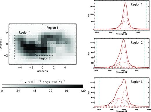
Hα emission per 0.52 × 0.52 arcsec2 spaxel. Three regions were defined across UM 448 over which summed spectra were extracted for analysis. On the right the Hα line profile from each summed region is shown, together with a two-component Gaussian fit. Blue dashed lines demarcate the wavelength range used for summing the flux. North is up and east is to the left.
The high spectral resolution and signal-to-noise ratio (S/N) of the data allow the identification of multiple velocity components in the majority of emission lines seen in the 300 spectra of UM 448 across the IFU aperture. Following the methods outlined in James et al. (2009) and Westmoquette et al. (2007), we utilized an automated fitting procedure called PAN (Peak ANalysis; Dimeo 2005) that allowed us to read in multiple spectra simultaneously, interactively specify initial parameters for a spectral line fit and then sequentially process each spectrum, fitting Gaussian profiles accordingly. The output consists of the χ2 value for the fit, the fit results for the continuum and each line's flux, centroid and FWHM, and the respective errors of these quantities which were propagated in all physical properties derived afterwards.4
Even though some low-S/N lines may in reality be composed of multiple emission components, it is often not statistically significant to fit anything more than a single Gaussian. In order to rigorously determine the optimum number of Gaussians required to fit each observed profile, we followed the likelihood ratio method outlined by Westmoquette, Smith & Gallagher (2011, their appendix A). S/N maps were first made for each emission line, taking the ratio of the integrated intensity of the line to that of the error array produced by the FLAMES pipeline, on a spaxel-by-spaxel basis. Single or multiple Gaussian profiles were then fitted to the emission lines, restricting the minimum FWHM to be the instrumental width (see Section 2). Suitable wavelength limits were defined for each line and continuum level fit. Further constraints were applied when fitting the [S ii] and [O ii] doublets: the wavelength difference between each line in the doublet was taken to be equal to the redshifted laboratory value when fitting the velocity component, and their FWHMs were set equal to one another.
The majority of high-S/N line profiles in the spectra of UM 448 are optimally fitted with a single narrow Gaussian (FWHM < 100 km s−1, hereafter component C1), a single underlying broad Gaussian component (FWHM 150–300 km s−1, hereafter C2) and a third narrow Gaussian which can appear either redshifted or blueshifted with respect to C1 (hereafter C3). In consideration of the different ‘features’ of each component (i.e. FWHM and/or velocity), we consider each component as being real, i.e. arising from gas with different physical conditions. Towards the outer regions of the galaxy, where the S/N decreases, the lines are optimally fitted with only C1 and C2 velocity components. Low-S/N emission lines (e.g. H8+He i λ3888) were optimally fitted with a single narrow Gaussian profile (C1). Fig. 3 shows the complex profile of the Hα line, along with the spatial distribution of its constituent velocity components.
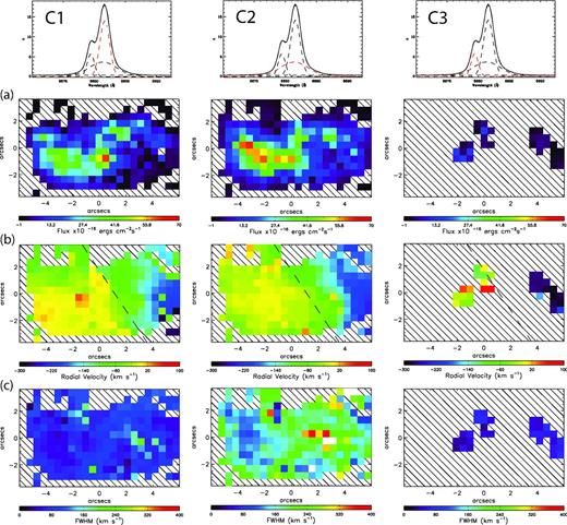
Maps of UM 448 in the Hα velocity components C1–C3: the top row shows an example three-component fit to the Hα line and the structure of the velocity component shown in red is displayed below; (a) flux in units of 10−16 erg s−1 cm−2 arcsec−2 per 0.52 × 0.52 arcsec2 spaxel; (b) radial velocity relative to the heliocentric systemic velocity of +5579 km s−1(the dashed line refers to the PA ∼ 36° rotation axis discussed in the text; (c) FWHM corrected for the instrumental PSF. See text for details. Maps are shown for S/N ≥ 10 in the integrated line profile. North is up and east is to the left.
Tables A1–A3 list measured FWHMs and observed and dereddened fluxes for the fitted Gaussian components of the detected emission lines across the three regions of massive SF defined in Fig. 2. The fluxes are for spectra summed over each region and are quoted relative to the flux of the corresponding Hβ component. They were corrected for reddening using the galactic reddening law of Howarth (1983) using c(Hβ) values derived from the Hα/Hβ and Hγ/Hβ line ratios of their corresponding components, weighted in a 3:1 ratio,5 respectively, in conjunction with theoretical Case B ratios from Storey & Hummer (1995). An extinction map was also derived using the Hα/Hβ and Hγ/Hβ emission line ratio maps and is shown in Fig. 4. This was computed using the integrated line profiles (i.e. C1+C2+C3) to obtain a global extinction view of the galaxy.
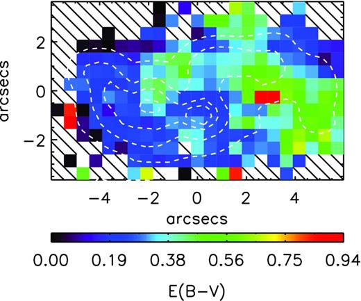
Map of E(B − V) for UM 448, derived from the integrated flux of H i emission lines. Integrated light Hα emission line contours are overlaid. North is up and east is to the left.
A Milky Way reddening of E(B − V) = 0.025 mag in the direction to UM 448 is indicated by the extinction maps of Schlegel, Finkbeiner & Davis (1998), corresponding to c(Hβ) = 0.036. Total c(Hβ) values applicable to the galaxy and its individual emission line components in each main aperture-region are listed in their respective tables (Tables A1–A3).
3.1 Hα maps
The Hα surface brightness of UM 448 (Fig. 3a) displays a horizontal ‘S’-shaped morphology, extending a total of ∼10 arcsec east to west, almost symmetrically about the FoV centre. The lower arm of the galaxy extends ∼5 arcsec to the east and contains the galaxy's peak Hα emission (corresponding to designated region 1). Based on our fitting method, the average surface brightness within region 1 can be decomposed to ∼1.8 × 10⁻¹⁴ and ∼2.8 × 10⁻¹⁴ erg cm−2 s−1 arcsec−2 for line components C1 and C2, respectively. The upper arm is seen to extend ∼5 arcsec in the opposite direction and displays an overall slightly lower surface brightness of ∼1.2 × 10⁻¹⁴ erg cm−2 s−1 arcsec−2 for both components. Component C3 appears in three separate regions: two regions either side of the central boundary region, i.e. between the two stellar components (see Fig. 1), and a third region along the most western part of the upper arm. C3 had an average surface brightness of ∼4.4 × 10⁻¹⁴ erg cm−2 s−1 arcsec−2. The total integrated Hα flux for UM 448 is 9.24 × 10⁻¹³ erg cm−2 s−1, which is in good agreement with the value of ∼11.5 × 10⁻¹³ erg cm−2 s−1 derived by Dopita et al. (2002) from narrow-band Hα imaging. Relative line intensities are listed in Tables A1–A3 for summed spectra over each of the three designated regions, for each separate velocity component.
The Hα velocity map (Fig. 3b) displays a rather similar radial velocity structure for both C1 and C2 components. Both show a smooth velocity distribution between +50 and −180 km s−1, which suggests solid body rotation within the galaxy. These maps can be used to derive an axis of rotation for the gaseous component of UM 448 along position angle (PA) ∼36° (shown as a dashed line in Fig. 3b). Interestingly, the alignment of this axis also divides the blue eastern ‘tail’ from the red, western part of the galaxy (Fig. 1). The radial velocity structure of component C3 is less straightforward than its counterparts. In the two regions near the centre of UM 448, the velocities range from −100 to +100 km s−1, whilst in the extreme west of the galaxy they are consistently negative down to −300 km s−1. The velocity structure there could be the signature of a discrete blueshifted outflow, which is perhaps related to the detached knots of emission present in the SuSI2 images ∼10 arcsec from the southwest corner of the Argus aperture (Fig. 1) – i.e. we are detecting fast-moving gas, kinematically decoupled from the main body of UM 448.
The maps of the Hα FWHM show a slight spatial correlation with the flux distribution (Fig. 3c). The eastern regions display decreased FWHMs for both the C1 and C2 line components, in comparison to the upper arm structure: the average FWHM for the lower arm is ∼40–60 km s−1 for C1 and 120–160 km s−1 for C2, which increases to ∼90–100 km s−1 and 200–240 km s−1, respectively, in the upper arm. Interestingly, the region of low FWHM is co-spatial with the main peak in flux within the eastern arm. If the overall appearance of UM 448 is indicative of a close encounter or merger of two systems, then it would make sense for the gas turbulence, and hence the FWHM, to increase as one approaches the transition region between the two colliding components (the blue/red interface in Fig. 1, right-hand panel). On the other hand, component C3 shows a typical FWHM of 70 km s−1suggesting an association with more orderly gas volumes.
3.2 Forbidden-line maps
Emission line maps of UM 448 in the light of the [O iii] [N ii] and [Ne iii] lines for the various velocity components are shown in Fig. 5. The morphology of [O iii] λ4959 is similar to that of Hα, with the surface brightness of the lower arm being higher by a factor of ∼2 than that of the upper arm (for component C1). In contrast, [N ii] displays a rather constant surface brightness throughout either arm, with a peak in emission within our designated region 2. For both [O iii] and [N ii] line component C2 displays a similar morphology to the C1 counterparts, as was the case with Hα. Component C3 of [O iii] λ4959 has a wider spatial extent than its counterpart in Hα. For [N ii] component C3 is seen to overlap roughly with the central and eastern regions observed for Hα-C3. In the central regions C3 shows symmetry approximately about the rotation axis defined in Fig 3b; this may a signature of an outflow, or it simply reflects the highly disturbed kinematics in the ‘collision zone’ of the merging galactic components at the region1/region2 aperture interface. [O iii] λ4363 has also been detected in velocity components C1 and C2 whose peak surface brightness is found within region 3 (see Fig. 6 for an example fit to the summed spectra across this region), whereas λ4959 peaks in region 1. This is mirrored in the high electron temperature of region 3 versus region 1 (see below). The [Ne iii] λ3868 emission also peaks within region 1, with more diffuse emission extending throughout regions 2 and 3.
![Dereddened intensity maps of UM 448 in [O iii] λ4959, [N ii] λ6584, [O iii] λ4363 and [Ne iii] λ3868 for the separate velocity components C1, C2 and C3. [O iii] λ4363 is shown after being rebinned by 1.5 × 1.5 spaxel and re-mapped on to the original grid (see the text for details). Only spaxels with S/N≥10 are shown for [O iii] λ4959 and [N ii] λ6584, ≥5 for [Ne iii] λ3868 and ≥1 for [O iii] λ4363. North is up and east is to the left.](https://oup.silverchair-cdn.com/oup/backfile/Content_public/Journal/mnras/428/1/10.1093/mnras/sts004/2/m_86fig5.jpeg?Expires=1750509854&Signature=BHnBCqlwedruyo3ugnr8BeN8l9khlNn-OeJViU4Sj6Qnjgz4KB7CvzwvWD9sz502-xqfEWEDhKYhTnTHgy15gkRsU1pc~n1C2t1qYPc-zpfTb24KwfdRZbZbwA6k2hU7522OOJ-Hsu-~6xhdg7PTu5d-JrqjGCCJuSZ5Nk0c40LFiyAOSeB2XT9cZn276DJkJhPBvHZStMHfPvfDJFvlbA1FMt36VImUh2MqwuXIjUY4sAibjBvlQh9R86o~2aRI8AvFsFg81Di19aAxthUAe5Ps1Q1Awa9ePr6kVRmB29fjRNhbh-g97sAh9dfFb5LBU57-LHMl~OF11vG9Ml2HZQ__&Key-Pair-Id=APKAIE5G5CRDK6RD3PGA)
Dereddened intensity maps of UM 448 in [O iii] λ4959, [N ii] λ6584, [O iii] λ4363 and [Ne iii] λ3868 for the separate velocity components C1, C2 and C3. [O iii] λ4363 is shown after being rebinned by 1.5 × 1.5 spaxel and re-mapped on to the original grid (see the text for details). Only spaxels with S/N≥10 are shown for [O iii] λ4959 and [N ii] λ6584, ≥5 for [Ne iii] λ3868 and ≥1 for [O iii] λ4363. North is up and east is to the left.
UM 448 is shown in the light of the [O ii] and [S ii] doublet lines in Fig. 7. Due to their relatively low S/N (compared to the H i Balmer lines and [O iii] λ4959), both doublets could be decomposed to only the C1 and C2 velocity components (Fig. 8). The [O ii] doublet, with a rest-wavelength separation of 2.783 Å was particularly hard to decompose into a narrow+broad component since the large FWHM of the component C2 would effectively merge the doublet into a single line. To alleviate this, each spaxel with a broad component [O ii] line detection was examined and only selected when there was sufficient S/N to allow for a deblended fit (see Fig. 8a). The larger wavelength separation of the [S ii] doublet allowed the broad component (C2) to be also fitted in relatively low-S/N spaxels (e.g. Fig. 8b), and was thus mapped more extensively than [O ii] (compare the bottom panels of Figs 7a and b). The [O ii] λ3727+λ3729 emission has a rather disjointed morphology compared to the integrated Hα surface brightness. The ratio of the [O ii] doublet components commonly used as a density diagnostic (Fig. 7, left-hand panels) displays negligible structure in relation to the overlaid Hα. In contrast to [O ii], the [S ii] λ6716+λ6731 doublet has a morphology that is more akin to Hα with three distinct peaks in flux. The λ6716/λ6731 ratio (Fig. 7, right-hand panels), which is also used as a density diagnostic, decreases in regions that align with the peaks in Hα emission, and this is indicative of increased electron density there.
![[O iii]λ4363 profile observed in the spectra summed over region 3, displaying a narrow (C1) plus broad (C2) component Gaussian profile. Flux, FWHM and velocity parameters for each component are listed in Table A3.](https://oup.silverchair-cdn.com/oup/backfile/Content_public/Journal/mnras/428/1/10.1093/mnras/sts004/2/m_86fig6.jpeg?Expires=1750509854&Signature=N~CXtJ~9587othOSQ7wZH8-DvHBy7OkpoIBN~QDQ7ZsZPjM5bfEd9ucC5Ha~ToN-n2rLeoKb4cvOEp7nGdpjxhgwmKsmwHWfL~bKaymJdQwfTnR~jjlQpr~0rtIeQQs1iuy3SDAFPn4iWUK-EY6DzeU1BDp5k6Z~78tBeb5oLaW4o111YauTOOU4I5Vew4J9NRNPUHEN5R~aQX3O-OHIK79OxwuNmwCHzpsiS3x4iQ-r4Uq8NP86sdn4JJTvBxaUbCwDIj8vDvpBJ388QPyD-SDiVxcTZRJz1PHWNrf3rLFf2bfGhOFBgQSldnDQSFTA43IA7z8BPtZklfeXuxajcQ__&Key-Pair-Id=APKAIE5G5CRDK6RD3PGA)
[O iii]λ4363 profile observed in the spectra summed over region 3, displaying a narrow (C1) plus broad (C2) component Gaussian profile. Flux, FWHM and velocity parameters for each component are listed in Table A3.
![Dereddened emission line maps of UM 448 in doublet ratios [O ii] λ3727/λ3729 (top-panel) and [O ii] λ6716/λ6731(bottom panel), in the separate C1 (narrow) and C2 (broad) velocity components, with integrated Hα emission line flux overlaid in contours. North is up and east is to the left.](https://oup.silverchair-cdn.com/oup/backfile/Content_public/Journal/mnras/428/1/10.1093/mnras/sts004/2/m_86fig7.jpeg?Expires=1750509854&Signature=emwJaP6JolVipcUIw9I2vGCuAfBegYfbogGO1EzwGer8nBVPETneldU6nuZ--1h-meeWfXgKV-jebzWMKvffvzvyM5ICnDuxSREfYsKUVSRlwEtB9NfObZVA8tlcOjrA3qI9wbhgFwKHtQhOrVP-NE-LEtoJaVJQIsOANLCIJZiyJRIuBptwGJXmjL0WAzNALVGH-1QGZSVXVuIeMCuRsibQfq9IVTC2lbdP9hSULP8sdWb-RdaiQWIDsLMZ50cFcU6P2w8cENjSnFgyBiWt7ZQQZWORYwGA0qmVnrnJ9Cht9nxYu~muFDsPlRLKFygnWiV6eWrUBSTYZKGYhu4f0A__&Key-Pair-Id=APKAIE5G5CRDK6RD3PGA)
Dereddened emission line maps of UM 448 in doublet ratios [O ii] λ3727/λ3729 (top-panel) and [O ii] λ6716/λ6731(bottom panel), in the separate C1 (narrow) and C2 (broad) velocity components, with integrated Hα emission line flux overlaid in contours. North is up and east is to the left.
![Example single-spaxel spectra and fits to the [O ii] λλ3727,3729 and [S ii] λλ6716,6731 lines. Flux is in units of ×10−16 erg cm−2 s−1 arcsec−2 Å−1 and wavelengths are in the rest frame.](https://oup.silverchair-cdn.com/oup/backfile/Content_public/Journal/mnras/428/1/10.1093/mnras/sts004/2/m_86fig8.jpeg?Expires=1750509854&Signature=yoyXhvfZx6lDRmzomXRPIAzCnLHrBQq6imjXyGNMKpT35Xq4pzAk847Hj38EyHL1IywTHOmQIktJ1HBrcuEZJkJqQnp0D5QJXpFKGmZnDFnxSwhg9p4FArnwqQd6wtBY0OguaCm~LESoLuxa0VDaCHnR6TZ2eNXO5AZR03vmJUCfqfISWFewMEqRf7kn5aGsK7epHTkliBprSg5ZDSSzaNhDtpINLYi2xfBO-Vpr9OfD7mWQEW8zWt9Sj6-w0stGm2AwXWVx4VtAixd0paR68K0AHfCGss0D4ALwxoLnKDvtFbgqIGiqpvDK2xsRAUu7xDKe3IH0DiPguuNYdyCCFg__&Key-Pair-Id=APKAIE5G5CRDK6RD3PGA)
Example single-spaxel spectra and fits to the [O ii] λλ3727,3729 and [S ii] λλ6716,6731 lines. Flux is in units of ×10−16 erg cm−2 s−1 arcsec−2 Å−1 and wavelengths are in the rest frame.
4 ELECTRON TEMPERATURE AND DENSITY
The [O iii] (λ5007 + λ4959)/λ4363 intensity ratios were used to determine electron temperatures. Two emission line doublets are available to determine the electron density, Ne: namely the [O ii] λ3726/λ3729 and [S ii] λ6716/λ6731 ratios. Te and Ne values were computed using iraf'sZONES task in the nebula package. This makes use of technique that derives both the temperature and the density by making simultaneous use of temperature- and density-sensitive line ratios. Atomic transition probabilities for O2+ and O+ were taken from Wiese, Fuhr & Deters (1996), whilst collision strengths were taken from Lennon & Burke (1994) and McLaughlin & Bell (1993), respectively. For [S ii] we used the transitional probabilities of Keenan et al. (1993) and the collisional strengths of Ramsbottom, Bell & Stafford (1996).
Where possible Te and Ne values were derived for each velocity component within each of the aperture regions defined in Fig. 2 and are listed in Table 2. The mean electron densities from the [S ii] and [O ii] ratios agree to within ∼20 per cent; the [O ii] density map is however significantly more noisy. The [S ii] densities were therefore adopted for the analysis.
Te and Ne maps computed for line components C1 and C2 are shown in Fig. 9, and mean values for each of the aperture regions 1–3 of Fig. 2 are listed in Table 2. Fig. 9 (left-hand panel) shows evidence for a small amount of Te variation throughout UM 448. Aperture regions 1 and 2 show temperatures of ∼12 000–13 000 K. Region 3 shows temperatures of 15 300 K for the narrow line component C1 and 10 200 K for the broad line component C2. Ne variations are also apparent and denser areas are correlated with peaks in Hα emission. Regions 1 and 2 have an average Ne ∼ 120-150 cm−3, whereas region 3 is only marginally denser with 200 cm−3.
![[O iii] electron temperature maps of UM 448 for C1 (narrow) and C2 (broad) velocity components. Overlaid circles represent the size of the Te uncertainty within each spaxel (percentage errors are scaled by the 0.52 arcsec diameter of a spaxel). North is up and east is to the left.](https://oup.silverchair-cdn.com/oup/backfile/Content_public/Journal/mnras/428/1/10.1093/mnras/sts004/2/m_86fig9.jpeg?Expires=1750509854&Signature=QYQocBXfYzeScVJqagO~DfkjlO5us11ah6aXmFA95i~z5MCOtuZMgKUQXOgZB6pejZTDsDE1-c-SPJh6i9od7r7RHVyZ~0aJ6Usvx96cEIWSt6ZPdVdapLqxKAlPYy7YtVFGti5ysJzNlHu3oBAhXD3dWdcpNIDf2umYJQKkaYp0YqndiqDt7H2F-YFuWvPWa3M65IVjX-MEns7l65BlYwAaInoAGw4I~E45bEZKHjDqXfPfXM83txBMDvngzM1ZLpBO7U7YgcoRjiHmoXgnbpn-O60S~WsJT8Ttop82Urz514Jp0xMI-QU93pAnRwk3RORf-2jub5wUj0inA4SR4g__&Key-Pair-Id=APKAIE5G5CRDK6RD3PGA)
[O iii] electron temperature maps of UM 448 for C1 (narrow) and C2 (broad) velocity components. Overlaid circles represent the size of the Te uncertainty within each spaxel (percentage errors are scaled by the 0.52 arcsec diameter of a spaxel). North is up and east is to the left.
5 CHEMICAL ABUNDANCES
Ionic abundance maps relative to H+ were created for the N+, O+, O2+, Ne2+ and S+ ions, using the λλ6584, 3727+3729, 4959, 3868 and 6717+6731 lines, respectively. Examples of the flux maps used in the derivation of these ionic abundance maps can be seen in Fig. 5. Abundances were calculated using the zones task in iraf, using the respective Te and Ne maps described above, with each FLAMES
spaxel treated as a distinct ‘nebular zone’ with its own set of physical conditions. These results were compared with those obtained using the multilevel ionic equilibrium program equib (originally written by I. D. Howarth and S. Adams at University College London), which comprises a different set of atomic data tables. Typical differences in the abundance ratios were found to be 5 per cent or less. To check the validity of using Te([O iii]) for the singularly ionized elements (N+, S+ and O+), we also computed abundance maps using a Te([O ii]) map [created using the relationship with Te([O iii]) described in Izotov et al. 2006. Discrepancies between the two temperatures were found to be low (∼100–400 K) and typical differences in ionic abundance were ∼2–7 per cent. These errors are lower than those caused by uncertainties in Te([O iii]) alone and we therefore do not include it as a source of error.
Ionic nitrogen, neon and sulphur abundances were converted into N/H, Ne/H and S/H abundances using ICFs from Kingsburgh & Barlow (1994). The O/H abundance was obtained by adding the O2+/H+ and O+/H+ abundance maps (i.e. assuming that the O3 +/H+ ratio is negligible). Since the [S iii] λ6312 line was not within the wavelength range of our data, the S2+/H+ abundance was estimated using the empirical relationship between the S2+ and S+ ionic fractions from the corrected equation (A38) of Kingsburgh & Barlow (1994), namely S2+/S+ = 4.677 × (O2 +/O+)0.433. The S/H results should therefore be considered with caution, but they are not at variance with those obtained using the ICF prescriptions of Izotov et al. (2006). O/H, N/H and log(N/O) abundance maps are shown in Fig. 10 and are described below. Regional abundances derived directly from taking error-weighted averages over the abundance maps are listed in Table 2.
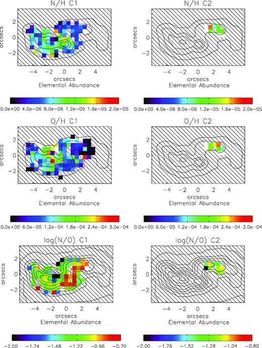
UM 448 nitrogen, oxygen and log(N/O) abundance maps for velocity components C1 and C2, with integrated light Hα emission line contours overlaid in dashed line. North is up and east is to the left.
5.1 Maps
The elemental oxygen abundance map shown in the middle panel of Fig. 10 displays a single peak whose location correlates with the peak in Hα relating to region 1. Minimal abundance variations are seen across UM 448, with a slightly decreasing oxygen abundance as one moves from regions 1–3, with an overall average abundance for C1 of 12 + log (O/H) = 8.15 ± 0.10. Adopting a solar oxygen abundance of 8.71 ± 0.1 relative to hydrogen (Scott et al. 2009), this corresponds to ∼0.28 Z⊙. This is comparable to the value obtained by Izotov & Thuan (1998, hereafter IT98), who measured an abundance of 12 + log(O/H) = 7.99 ± 0.04. The C2 velocity component displays a higher oxygen abundance than the C1 component gas within region 3 by ∼0.4 dex, which, judging from the agreement between C1 and C2 [O iii] 4959 Å flux (Fig. 5), is mostly attributable to the Te being ∼5000 K cooler (if the C1 region was instead much denser but of similar oxygen abundance to the gas sampled by the C2 line component, one might expect the λ4959/Hβ C1 ratio to be much smaller something which is not observed – Table A3).
The top panel of Fig. 10 shows the N/H abundance across UM 448. The C1 peak in nitrogen abundance is offset from that of oxygen, peaking at the location of region 2 with an average N/H ratio of 1.04 ± 0.01 × 10⁻⁵. For region 1 it is slightly lower at 9.40 ± 0.02 × 10⁻⁶ and for region 3 even lower at 7.00 ± 0.03 × 10⁻⁶. The C2 component gas in region 3 has a nitrogen abundance that is higher than its C1 counterpart by a factor of 2. As a result, there is a peak in the N/O ratio within UM 448 located at region 2, which can be seen in the bottom panel of Fig. 10. For C1, regions 1 and 3 agree with an average of log(N/O) ∼ −1.23 ± 0.04, whereas region 2 has an average (N/O) ratio of ∼ −1.03 ± 0.05. The map of log(N/O) shows that this peak actually reaches ∼ −0.80 at the precise location of region 2 (as can be seen from the Hα contours). The N/O ratio of the (broad) C2 component gas in region 3 (∼ −1.26 ± 0.13) is in good agreement with the average N/O of C1 gas in that region. The long-slit study by IT98 measured an N/H ratio of 9.5 ± 2.0 × 10⁻⁶, in agreement with the averages of regions 1 and 2 derived from the N/H map shown in Fig. 10. The average C1 N/O ratios for region 3 is slightly higher (by ∼0.2 dex) than those of other galaxies of similar oxygen metallicity (see López-Sánchez & Esteban 2010, their fig. 11). They are, however, consistent within the uncertainties. Region 2, however, has a higher value than the average value of ∼ −1.4 ± 0.2 expected for its metallicity, even when taking the uncertainties into consideration, for both the averaged value of region 2 and on a spaxel-by-spaxel basis. For this region we do observe the factor of ∼3 nitrogen excess reported by Pustilnik et al. (2004).
The Ne/H and S/H abundance distributions throughout UM 448 for the narrow (C1) emission line component show only minimal abundance variations in relation to the Hα emission. Ne/H values averaged over each region range from ∼2.06 to 6.55 × 10⁻⁵, with the highest Ne/H abundance aligning with region 2. The Ne/O ratios of region 1 and 3 are typical for those expected by BCGs at similar metallicities; the averaged region values lie within the reported range of log(Ne/O) ∼ −0.9 to −0.7 (Izotov et al. 2006). However, the Ne/O ratio for region 2 is ∼0.5 dex higher than the expected Ne/O value. Calculations of Ne/H were also made using the Ne2+ ICF of Izotov et al. (2006); however, the Ne/O ratio for region 2 remained ∼0.2 dex higher than the expected value. The S/H distribution across UM 448 is relatively constant for the C1 and C2 gas components, with each region displaying averages within the range of ∼4.7–7.4 × 10⁻⁶. The C1 S/O ratio for all regions is slightly higher than expected for BCGs, log(S/O) ∼ −1.9 to −1.5 (Izotov et al. 2006), and the S/O value C2 component in region 3 lies at the upper limit of this average.
5.2 Comparison of spatially resolved and global spectra abundances
Also listed in Table 2 are the Te, Ne, ionic and elemental abundances derived from summed spectra over the entire galaxy (using line fluxes listed in Table 3). This particular set of results allows us to assess if global galaxy spectra can reliably represent the physical properties of its interstellar medium (ISM). For example, values derived from long-slit observations may contain luminosity-weighted fluxes and consequently erroneous ratios, or large apertures may include a mixture of gas with different ionization conditions and/or metallicities. This question was addressed by Kobulnicky, Kennicutt & Pizagno (1999) to assess whether global emission-line spectra can be depended upon to reliably recover the chemical properties of distant star-forming galaxies. Overall, they find that when using direct-method techniques, global spectra can give an accurate representation of the oxygen abundances derived from individual H ii regions, but only after applying a correction of Δ(O/H) = 0.1 to the global spectra results. In addition to this, Pilyugin et al. (2012) found that oxygen abundances were systematically underestimated (and N/O consequently overestimated) when using global Sloan Digital Sky Survey (SDSS) spectra of H ii regions with different physical properties.
UM 448 fluxes and dereddened line intensities [both relative to F(Hβ) = I(Hβ) = 100] for summed spectra over all of UM 448. Line fluxes were extinction corrected using the c(Hβ) values shown at the bottom of the table, calculated from the relative Hα, Hβ and Hγ fluxes. The line intensities listed here were used for summed-spectra Te and Ne diagnostics and regional ionic abundance calculations listed in Table 2.
| Fλ | Iλ | |
|---|---|---|
| [O ii] λ3727 | 98.02 ± 1.18 | 125.40 ± 6.20 |
| [O ii] λ3729 | 135.65 ± 1.43 | 173.55 ± 8.52 |
| [Ne iii] λ3868 | 23.41 ± 1.71 | 29.24 ± 2.54 |
| H8+He i λ3888 | 15.47 ± 2.24 | 19.26 ± 2.93 |
| Hδ | 21.57 ± 1.21 | 25.70 ± 1.85 |
| Hγ | 43.33 ± 0.83 | 48.96 ± 2.31 |
| [O iii] λ4363 | 1.90 ± 0.19 | 2.14 ± 0.23 |
| He i λ4471 | 4.50 ± 0.49 | 4.94 ± 0.57 |
| Hβ | 100.00 ± 0.99 | 100.00 ± 3.94 |
| [O iii] λ4959 | 91.86 ± 1.66 | 89.76 ± 3.71 |
| [N ii] λ6548 | 15.83 ± 0.52 | 11.66 ± 0.49 |
| Hα | 407.05 ± 13.27 | 301.47 ± 12.62 |
| [N ii] λ6584 | 58.55 ± 0.51 | 42.91 ± 1.17 |
| He i λ6678 | 2.86 ± 0.06 | 2.07 ± 0.07 |
| [S ii] λ6716 | 49.17 ± 0.44 | 35.38 ± 0.94 |
| [S ii] λ6731 | 36.07 ± 0.34 | 25.95 ± 0.70 |
| c(Hβ) | 0.42 ± 0.02 | |
| F(Hβ) | 24.48 ± 0.17 | |
Ionic and elemental abundances for UM 448, with the corresponding Te and Ne used in their derivation. Columns 2–5 refer to abundances derived from maps, weight-averaged over regions defined in Fig. 2. Column 6 refers to Te, Ne and abundances derived from spectra integrated over UM 448 (corresponding fluxes are listed in Table 3). All ionization correction factors (ICFs) are taken from Kingsburgh & Barlow (1994). S/H ratios were calculated using the ICF(S) values listed along with a predicted value of S2+ (see text for details).
| Region 1 | Region 2 | Region 3 | Integrated spectrum | ||
|---|---|---|---|---|---|
| C1 | C1 | C1 | C2 | All components | |
| (1) | (2) | (3) | (4) | (5) | (6) |
| Te | 12220 ± 60 | 13020 ± 150 | 15340 ± 190 | 10230 ± 210 | 13,610 ± 560 |
| Ne | 100 ± 25 | 80 ± 35 | 115 ± 35 | 95 ± 30 | 40 ± 6 |
| O+/H+ × 105 | 7.24 ± 0.27 | 6.50 ± 0.53 | 5.23 ± 0.53 | 15.49 ± 1.55 | 12.25 ± 0.62 |
| O2+/H+ × 105 | 9.00 ± 0.31 | 4.56 ± 0.31 | 5.24 ± 0.43 | 10.91 ± 0.33 | 9.40 ± 0.48 |
| O/H × 104 | 1.62 ± 0.08 | 1.11 ± 0.12 | 1.05 ± 0.14 | 2.64 ± 0.28 | 2.16 ± 0.16 |
| 12+log(O/H) | 8.21 ± 0.05 | 8.04 ± 0.11 | 8.02 ± 0.13 | 8.42 ± 0.10 | 8.34 ± 0.07 |
| Z/ Z⊙ | 0.32 ± 0.02 | 0.22 ± 0.02 | 0.20 ± 0.03 | 0.51 ± 0.05 | 0.42 ± 0.03 |
| N+/H+ × 106 | 4.19 ± 0.14 | 6.08 ± 0.28 | 3.49 ± 0.21 | 8.45 ± 0.85 | 8.74 ± 0.76 |
| ICF(N) | 2.24 | 1.70 | 2.00 | 1.70 | 1.77 |
| N/H × 106 | 9.40 ± 0.66 | 10.35 ± 1.46 | 7.00 ± 1.24 | 14.40 ± 2.53 | 15.44 ± 1.91 |
| log(N/O) | −1.24 ± 0.05 | −1.03 ± 0.09 | −1.18 ± 0.12 | −1.26 ± 0.14 | −1.15 ± 0.10 |
| Ne2 +/H+ × 105 | 2.10 ± 0.12 | 2.70 ± 0.5 | 1.03 ± 0.13 | – | 3.16 ± 0.63 |
| ICF(Ne) | 1.80 | 2.42 | 2.00 | – | 2.30 |
| Ne/H × 105 | 3.78 ± 0.31 | 6.55 ± 0.1.46 | 2.06 ± 0.41 | – | 7.27 ± 1.59 |
| log(Ne/O) | −0.63 ± 0.10 | −0.23 ± 0.25 | −0.71 ± 0.24 | – | −0.47 ± 0.20 |
| S+/H+ × 106 | 1.11 ± 0.04 | 0.92 ± 0.05 | 1.06 ± 0.06 | 1.43 ± 0.09 | 1.87 ± 0.17 |
| ICF(S) | 1.06 | 1.02 | 1.04 | 1.02 | 1.03 |
| S/H × 106 | 7.23 ± 0.45 | 4.75 ± 0.63 | 6.30 ± 1.05 | 7.35 ± 1.06 | 9.93 ± 0.92 |
| log(S/O) | −1.35 ± 0.08 | −1.37 ± 0.17 | −1.22 ± 0.21 | −1.56 ± 0.18 | −1.34 ± 0.12 |
For UM 448, the temperature derived from the integrated spectrum is in agreement with the flux-weighted mean Te across the three regions (14010 ± 2100 K), suggesting that the integrated [O iii] ratio may have been more heavily weighted by areas of stronger [O iii] λ4363 emission. The oxygen abundance from the integrated spectrum, 12 + log(O/H) = 8.34 ± 0.07, is higher than all C1 component values, suggesting that it may be weighted towards the high O/H abundance seen in the C2 component of region 2. Being +0.18 dex higher than the flux-weighted average of the three regions (12+log(O/H) = 8.16 ± 0.18), the globally derived (i.e. derived from the integrated spectrum) O/H is not fully representative of the emission from the whole galaxy, even after applying the correction suggested by Kobulnicky et al. (1999). Nitrogen, too, displays a higher abundance when derived from the summed spectrum rather than the regional averages, and results in a (log) nitrogen-to-oxygen ratio of −1.15, which is approximately the expected value at this metallicity. The Ne/H abundance ratio from the integrated spectrum is almost a factor of 2 higher than the flux-weighted average of the three regions (∼2.14 × 10⁻⁵), whilst the log(Ne/O) ratio is in good agreement. The same applies for the S/H abundance, although less severe, where the globally derived S/H ratio is a factor of ∼1.5 higher than the flux-weighted average S/H across the three regions, but the log(S/O) value is in agreement between the two methods.
Comparisons can also be made with the results from a long-slit study by IT98, which utilized summed spectra over a 2 × 7 arcsec2 region ‘across the brightest region of the galaxy’. From this spectrum they derive an Te of 12100 ± 500 K (in line with the C1 component values of our region 1), O, N, Ne and S abundances that are systematically lower than those derived from our summed spectrum and abundances relative to oxygen that are in relatively good agreement within the uncertainties. However, without knowing the exact positioning of this slit, a truly meaningful comparison cannot be made.
Overall it can be said that whilst abundance ratios of heavy elements can be reasonably well obtained by summed spectra and/or long-slit observations, the ionic and elemental abundances relative to hydrogen are not well reproduced; this may be because the former properties do not have a very severe sensitivity to Te biases, while the latter do. This is in addition to the fact that, in contrast to IFS, global properties derived from light-averaged methods cannot resolve abundance variations and any potential sites of enrichment are being averaged out. Of course, uncertainties will still exist within IFU observations due to averaging along the line of sight of individual spaxels; this is something that can only be remedied with the development of higher spectral resolution IFUs.
6 STELLAR POPULATIONS
6.1 Age of the stellar population
Fig. 11 shows a combined New Technology Telescope (NTT)-SuSI2 R-, V- and B-band image that shows the stellar continuum within UM 448. Overlaid on the top panel are the contours of the continuum emission in the Hα spectral vicinity (∼6 Å windows either side of the line) that are in good agreement with the morphology of the broad-band images. In the bottom panel we show the same broad-band images with the Hα integrated-light emission line contours. Significant differences between the morphology of the ionized gas emission and that of the stellar continuum are clearly apparent, especially in the top, western ‘arm’. A strong continuum peak can be seen, which is not mirrored by the Hα emission, suggesting that a strong stellar component exists within this region. From the broad-band colour image shown in Fig. 1 it can be seen that this peak in continuum is red in colour, signifying an older stellar population than that seen in the bluer, eastern ‘arm’. Such a distinct, two-component stellar structure, in conjunction with the difference in radial velocity between them (see Fig. 3b), supports the interpretation that UM 448 is a merging system comprised of two galaxies, with very different ages. Spectra summed over this continuum peak region (represented by the white-dashed box overlaid in Fig. 11, bottom panel) do not reveal any stellar absorption features around the Hα, Hβ, Hγ or Hδ lines; however, Ca ii H, K (λλ3970, 3934) interstellar absorption features were detected.
NTT-SuSI2 combined R-, V- and B-band images of UM 448 with contours showing the continuum near Hα (top panel) and integrated Hα emission (bottom panel; see Fig. 3 for maps of the separated emission line components). North is up and east is to the left. Hα contours are shown for the range 35.0–128.6 in steps of 22.0, in flux units of 10−16 erg s−1 cm−2 arcsec−2. The continuum peak region is represented by the white-dashed box; spectra were summed over this region to investigate stellar absorption features and averages in EW(Hβ).
The age of a young population in a galaxy can be estimated using hydrogen recombination lines, since they provide an estimate of the ionizing flux present, assuming a radiation-bounded H ii region (Schaerer & Vacca 1998). In particular, the equivalent width (EW) of Hβ can be used as an age indicator of the ionizing stellar population at a given metallicity. A map of EW(Hβ) for UM 448 can be seen in Fig. 12. Whilst there are no clear peaks in EW(Hβ), the main region of decreased EW correlates with the largest peak in continuum emission (red contours) and that corresponds to region 3.
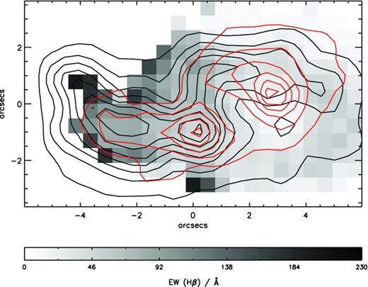
Map of the equivalent width of Hβ across UM 448. Overlaid red lines are contours of Hβ-region continuum; black lines are Hβ flux contours from Fig. 2.
Following the method outlined by James et al. (2010), we can use this map, in conjunction with the metallicity map described in Section 5, to estimate the age of the most recent star-forming episodes throughout UM 448, by comparing the regional observed average EW(Hβ) values with those predicted by the spectral synthesis code starburst99 (Leitherer et al. 1999). For the models we chose a metallicity of 0.2 Z⊙, the closest representative to the weighted average metallicity of UM 448 (∼0.25 Z⊙, derived from regional averages), together with assumptions of an instantaneous burst with a Salpeter initial mass function (IMF), a total starburst mass of 1 × 10⁶ M⊙, a 100 M⊙ stellar upper mass limit (which approximates the classical Salpeter 1955 IMF). Models were run for Geneva tracks with ‘high’ mass loss rates and Padova tracks with thermally pulsing asymptotic giant branch (AGB) stars included. For each of these evolutionary tracks, two types of model atmosphere were used: first the Pauldrach–Hillier (PH) and second Lejeune–Schmutz (LS). The latter was chosen because it incorporates stars with strong winds, which would be representative of the WR population within the galaxy (if present). The stellar ages predicted by each model and the observed average EW(Hβ) within each peak emission region in UM 448 were derived from Fig. 13 and are listed in Table 4.
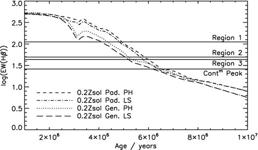
EW(Hβ) as a function of age, as predicted by the starburst99 code for metallicities of 0.2 Z⊙ using a combination of Geneva or Padova stellar evolutionary tracks and Lejeune–Schmutz (LS) or Pauldrach–Hillier (PH) model atmospheres. The observed average EW(Hβ)’s for each star-forming region in UM 448, along with the peak in continuum highlighted in Fig. 11 (bottom panel), are overlaid (solid line).
Age of the latest star formation episode and current star formation rates.
| Starburst ages (Myr) | ||||
|---|---|---|---|---|
| Model | Reg. 1 | Reg. 2 | Reg. 3 | Contm peak |
| Padova-AGB PH | 5.06 ± 0.24 | 5.86 ± 0.13 | 6.36 ± 0.48 | 8.61 ± 0.74 |
| Padova-AGB LH | 4.96 ± 0.24 | 5.66 ± 0.13 | 6.01 ± 0.33 | 8.51 ± 0.79 |
| Geneva high PH | 4.41 ± 0.27 | 5.31 ± 0.16 | 5.91 ± 0.56 | 7.91 ± 0.74 |
| Geneva high LS | 3.86 ± 0.48 | 5.11 ± 0.16 | 5.61 ± 0.50 | 7.76 ± 0.82 |
| Star formation rates (M⊙ yr−1) | ||||
| SFR(Hα)a | 1.49 ± 0.03 | 0.75 ± 0.02 | 0.90 ± 0.02 | 0.34 ± 0.01 |
| SFR(Hα)b | 0.82 ± 0.02 | 0.41 ± 0.01 | 0.50 ± 0.01 | 0.18 ± 0.01 |
The difference between the ages predicted by the Geneva and Padova stellar evolutionary tracks is relatively small, with the Geneva tracks predicting lower ages by up to 23 per cent. The difference in ages predicted by the PH and LS atmospheres is smaller still, with LS predicting lower ages by ∼5 per cent. We cannot comment on which atmosphere model is more appropriate given that the existence of WR stars within UM 448 is not confirmed by the current study; hence we adopt average stellar ages from the four model combinations. The current (instantaneous) star formation rates (SFRs) based on the Hα luminosities were calculated following Kennicutt (1998) and are given in Table 4. SFRs corrected for the subsolar metallicities are also given, derived following the methods outlined by Bicker & Fritze-v. Alvensleben (2005).
Regions 1–3 contain ionizing stellar populations with average ages of 4.6, 5.5 and 6.0 Myr, respectively, and the region of peaked continuum (Fig. 11) has an average age of 8.2 Myr (Table 4). Since region 1 shows the highest ionizing flux, we would expect it to contain the youngest stellar population. It is notable that the ages of the stellar population increase through regions 1–3 as one moves away from the blue continuum peak (Fig. 1). However, the SFR does not show a smooth decrease in the same direction, decreasing slightly for region 2 before increasing again for region 3. Interestingly, and not surprisingly, the main red-coloured stellar continuum peak (Figs 1 and 11) displays an increase in age of almost 4 Myr from the blue continuum peak (region 1) and a much decreased SFR compared to the three main regions of SF. Using narrow-band Hα imaging, Dopita et al. (2002) derived a total SFR of 6.6 M⊙ yr−1, which is in good agreement with that derived from our total Hα flux, 5.0 M⊙ yr−1. Accounting for its ∼0.2 Z⊙ metallicity, this translates to 2.8 M⊙ yr−1. The evidence suggests that UM 448 is made up of two separate bodies undergoing a merger: the first is sampled by our aperture regions 1 and 2, where relatively recent bursts of SF have occurred. The second body with which it is merging may be an older galaxy (represented by the red continuum peak) sampled by aperture region 3, within which the collision could have triggered SF, hence an increased SFR but overall age that is representative of an aggregate old+young population.
6.2 WR stars and N enrichment
Contrary to the conclusions of previous long-slit studies (Masegosa, Moles & del Olmo 1991; Schaerer, Contini & Pindao 1999, and references therein) and in agreement with Guseva et al. (2000), our FLAMES IFU spectra do not reveal evidence of ‘strong’ WR emission bands at ∼4640–4686 Å. Unfortunately, the C iv 5801, 5812 Å feature is not included in our wavelength coverage, although these features are usually significantly weaker than the ∼4686 Å feature. We find no evidence of a WR population in our single spaxel spectra and only minimal evidence in our spectra summed over the entire galaxy. When searching for WR features one must consider the width of the extraction aperture, which can sometimes be too large and dilute weak WR features by the continuum flux (López-Sánchez & Esteban 2008). This has indeed been the case for several other BCGs, where previous reports of detections of WR features in long-slit spectra were not confirmed by IFU spectra (e.g. James et al. 2010; Pérez-Montero et al. 2011). We therefore also examined the spectra summed over each individual region (Fig. 2), which are shown in Fig. 14.
![Sections of continuum-subtracted FLAMES IFU spectra, showing the blue ‘WR bump’ region within summed spectra over the entire galaxy and separate aperture regions 1, 2 and 3 (see Fig. 2). There are minimal detections of WR emission features within both the spectra summed over the entire galaxy and also each of the individual aperture region spectra. Overlaid are the estimates of 4000 ± 1100, 900 ± 600, 300 ± 600 and 1300 ± 400 WN (5–6) stars (solid red line), for the entire galaxy and regions 1–3, respectively, using the templates of Crowther & Hadfield (2006), along with the 1σ errors (dashed red line). Vertical dashed lines indicate the location of [Fe iii] 4658 Å and a weak, narrow, He ii emission line at 4686 Å. The dashed horizontal lines in the plots show the zero flux levels.](https://oup.silverchair-cdn.com/oup/backfile/Content_public/Journal/mnras/428/1/10.1093/mnras/sts004/2/m_86fig14.jpeg?Expires=1750509854&Signature=NO3rNmQNh5aJE7pfkKXAao6Yume8POFwhyp0TlbIVuRHEU503LnlXfgmGwRzjRtNwLLK~rnvSy4QnHlfyXHXdnZZDh7JpezBIWe-6ajIxDh~gs4pU321DyaEDX0vfs8tDH9LGMkmYPr9aomrnzYX0ozL8BxjSpGrLPnqmVbgGzLiZ96L5HROt4AsdNn1rmIAf9HawZxu2EYKueWyzhvF-8wgxcKKIK97sf3PCDCi5hvZmt4B79ijuQl4m4U0LEtLbN3pAhvEqTe0Dyi9z0yURVYpYfBsNYT-D82uC6kWHtTDmUOr89-B3FukFMhZvAf7-IKAXyLQ9viuf2j5xLdtug__&Key-Pair-Id=APKAIE5G5CRDK6RD3PGA)
Sections of continuum-subtracted FLAMES IFU spectra, showing the blue ‘WR bump’ region within summed spectra over the entire galaxy and separate aperture regions 1, 2 and 3 (see Fig. 2). There are minimal detections of WR emission features within both the spectra summed over the entire galaxy and also each of the individual aperture region spectra. Overlaid are the estimates of 4000 ± 1100, 900 ± 600, 300 ± 600 and 1300 ± 400 WN (5–6) stars (solid red line), for the entire galaxy and regions 1–3, respectively, using the templates of Crowther & Hadfield (2006), along with the 1σ errors (dashed red line). Vertical dashed lines indicate the location of [Fe iii] 4658 Å and a weak, narrow, He ii emission line at 4686 Å. The dashed horizontal lines in the plots show the zero flux levels.
In order to determine the number of WR stars from the strength of the 4640–4690 Å feature for the summed spectra over regions 1–3, the local continuum was subtracted. A linear interpolation to the continuum from both sides of the 4640–4686 Å region was employed based on the mean flux in a blue region (rest wavelengths 4609–4640 Å, avoiding the [Fe iii] emission line and possible C iii absorption at 4647 Å) and a red region (4711–4742 Å). Utilizing an Large Magellanic Cloud (LMC) WR (WN 5–6) spectral template from Crowther & Hadfield (2006), the best match of the scaled WR star flux to the flux over the observed broad 4686 Å region was determined by minimizing χ2 over the peak of the WR feature, typically 4670–4900 Å. Since errors were available on the flux points, these were used to generate a series of Monte Carlo realizations of each region spectrum and the WR template flux was best fitted to each. The distribution the WR template flux to each realization was fitted by a Gaussian enabling the 1σ errors to be estimated. The flux of the WR template was then converted into the number of WR stars allowing for the distance of UM 448. We estimate 900 ± 600, 300 ± 600 and 1300 ± 400 WN stars for regions 1–3, respectively. A total population of 4000 ± 1100 WN stars was estimated applying the same procedure for the summed spectrum for the entire galaxy. These error estimates are based purely on the flux errors and do not take into account any systematic error arising from the, necessarily simplified, removal of a linear continuum under the WR line. The WR template fits and the error ranges for the summed spectra over the entire galaxy and the three regions 1–3 are shown in Fig. 14. However, considering the large uncertainties, the existence of a WR population within UM 448 is still considered to be speculative and as a result, we cannot conclude that the Δlog(N/O) ∼ +0.6 dex excess observed in region 2 is due to nitrogen enrichment from WR stars.
However, following the methodology outlined in Pérez-Montero et al. (2011), we can use the size of the N-enriched region in UM 448 (∼1.6 × 1.6 arcsec2 = 0.6 kpc2) in region 2 as a scalelength to assess whether the reported WR stars could be the actual source of this N pollution. Using modelled chemical yields at ∼0.2 Z⊙, those authors study the effects of elements ejected into the ISM via winds as a function of time and pollution radii (see Pérez-Montero et al. 2011, section 4.3 for a full description of the model parameters). After ∼4 Myr, the appearance of WR star winds increases the N/O ratio, where the value of N/O ratio only reaches that of region 2 at radii much lower (e.g. r = 10 or 100 pc) than those measured from our IFU observations. Therefore, although WR stars have been detected in previous long-slit studies, and are tentatively detected here, the high N/O ratio observed within region 2 is not likely produced by the pollution from stellar wind ejecta coming from WR stars. Instead, this enrichment may be related to other global processes occurring within UM 448, namely the likely interaction and/or merger between two bodies as inferred from the SuSI2 images and radial velocity maps. Studies suggest that interacting galaxies fall ≳0.2 dex below the mass–metallicity relation of normal galaxies due to tidally induced large-scale inflow of metal-poor gas to the galaxies’ central regions (e.g. Kewley, Geller & Barton 2006; Michel-Dansac et al. 2008; Peeples, Pogge & Stanek 2009; Rupke, Kewley & Chien 2010; Torrey et al. 2012). In addition, models by Köppen & Hensler (2005) have shown that a rapid decrease in oxygen abundance during an episode of massive and rapid accretion of metal-poor gas is followed by a slower evolution which leads to the closed-box relation, thus forming a loop in the N/O–O/H diagram. Such a scenario, in conjunction with metal-rich gas loss driven by supernova winds, has been suggested by Amorín, Pérez-Montero & Vílchez (2010) to explain the systematically large N/O ratio found within green pea galaxies.
7 SUMMARY AND CONCLUSIONS
We have analysed FLAMES-IFU IFS of the BCG UM 448 and studied its morphology by creating monochromatic emission line maps. This system shows signs of interaction and/or perturbation and it is possibly undergoing a merger. Based on the emission line morphology, we defined three regions of high Hα surface brightness which we use to derive error-weighted averages of the physical and chemical conditions across UM 448. Region 1 is to the east and corresponds to the tidal tail, region 3 extends towards to the upper west and region 2 lies between them. UM 448 exhibits complex emission line profiles, with most lines consisting of a narrow, central component and an underlying broad component, and a third, narrow blueshifted component is also detected in regions 2 and 3.
Abundance ratio maps of O/H, N/H, Ne/H and S/H were created based on the direct method of estimating electron temperatures from the [O iii] λ4363/λ4959 line ratio. Minimal variance in oxygen abundance is seen across UM 448 for the narrow velocity component, with an average abundance of 12+log(O/H) = 8.15 ± 0.1. However, in an area of UM 448 where the [O iii] 4363 Å line is resolved into a narrow+broad component, an ∼0.4 dex increase in oxygen abundance attributable to a decrease in Te of ∼5000 K is found in the broad-line region. We detect the previously reported high N/O ratio, with Δlog(N/O) ∼ +0.4, in our aperture region 2 only, spatially coincident with a peak in nitrogen abundance. Abundances derived from an integrated spectrum of UM 448 are not a reliable representation of the ionic and elemental abundances throughout UM 448, which may be a consequence of the variance in Te throughout the nebular emission line components of UM 448 detected in these integral field spectra. However, abundances relative to oxygen from the two methods (i.e. map-based averages versus integrated spectra) are consistent within the uncertainties. These results are significant when assessing the reliability of abundances derived from long-slit and integrated spectra of both nearby and high-redshift star-forming galaxies that do not contain homogeneous ionization conditions and/or metallicities.
Continuum images of UM 448 display a rather different morphology to those of the emission lines, with a peak in stellar light situated in between the second and third custom-aperture regions. The colour of this continuum peak (from SuSI2 broad-band images) shows signs of a red, older stellar population in contrast to a younger, bluer stellar population situated in the eastern body of UM 448. SFRs were computed from the Hα line luminosities within each sampled star-forming region and the ages of the last major SF episode were estimated by fitting the observed Balmer line EWs with starburst99 models. The two merging sections of UM 448 have SFRs that differ by a factor of ∼5 and starburst episodes separated by 4 Myr, providing evidence of a distinct age gradient between the two components. The latest major SF event took place ∼4.5 Myr ago in the largest merging component, and has been producing stars at a rate of 0.8 M⊙ yr−1.
Finally, we do not detect the previously reported ‘strong’ WR signatures in UM 448, on a single-spaxel, regional or global scale (Masegosa et al. 1991; Schaerer et al. 1999). Using the 4686 Å feature we tentatively estimate that ∼4000 WN stars may be present within UM 448. In consideration of the physical size of increased N/O seen within UM 448 (∼0.6 kpc2), we find that WR stars alone cannot be responsible for the region of N enrichment within UM 448. Thus being, another chemical evolution scenario (e.g. inflow of metal-poor gas due to interaction or merger scenario, as the morphology and dynamics of UM 448 suggest) is required to explain this enhancement. Since there is no strong evidence in support of these scenarios (although broad component emission is suggestive of an outflow, the N enrichment is seen in the narrow component only), more observations, at higher sensitivity, are needed of this intriguing system. In relation to other high N/O BCGs, this chemodynamical study supports its membership within the anomalous subset and, along with other spatially resolved spectroscopic studies of high N/O galaxies, demonstrates the benefits that this method can have in both isolating the enrichment and aiding our understanding of the processes that cause it.
We would like to thank the FLAMES staff at Paranal and Garching for scheduling and taking these service mode observations (programme 083.B-0336B; PI: B. L. James). We appreciate discussions with Alessandra Aloisi regarding theories of primary/secondary nitrogen production. We also thank the referee for the useful comments that have significantly improved the first submitted version of this manuscript. YGT acknowledges the award of a Marie Curie intra-European Fellowship within the Seventh European Community Framework Programme (grant agreement PIEF-GA-2009-236486). BLJ acknowledges support from an STScI-DDRF travel grant used to visit collaborators of this study. This research made use of the NASA ADS and NED data bases.
SuSI2 images were obtained from the ESO archive, with total exposure times of 1200, 1200, 1800 and 2700 s, average airmasses of 1.34, 1.28, 1.22 and 1.17 and image qualities of 0.75, 0.93, 0.87 and 0.56 arcsec FWHM for the R-, V-, B- and U-band images, respectively. The average image quality of the images is ∼0.78 arcsec FWHM. WCS information was assigned via position matching with GSC2. Other than aligning and median-combining the separate frames using iraf’s imalign and imcombine, respectively, no additional reduction was performed on the images.
The girbldrs pipeline is provided by the Geneva Observatory http://girbldrs.sourceforge.net.
iraf (Image Reduction and Analysis Facility) is distributed by the National Optical Astronomy Observatory, which is operated by the Association of Universities for Research in Astronomy.
The uncertainties output by the pipeline were used as the starting point of the error analysis; they also include uncertainties from the flat-fielding and the geometric correction of the spectra and not just photon noise (Blecha & Simond 2004).
An exception was made for region 3 where the low S/N of Hγ prohibited the robust decomposition into the three components observed in Hα and Hβ. Therefore, only the Hα/Hβ line ratio was used for the calculation of c(Hβ) for this region.
REFERENCES
APPENDIX A: REGIONAL OBSERVED FLUXES AND LINE INTENSITIES
Tables A1–A3 list the observed fluxes and dereddened line intensities derived from summed spectra over the regions defined in Fig. 2. Fluxes are given for each separate velocity component (C1–C3), along with its dereddened line intensity and FWHM.
UM 448 regional fluxes and dereddened line intensities [both relative to F(Hβ) = I(Hβ) = 100] and FWHMs (in km s−1) for summed spectra over region 1 (as defined in Fig. 2). Line fluxes were extinction corrected using the c(Hβ) values shown at the bottom of the table, calculated from the relative Hα, Hβ and Hγ fluxes. F(Hβ) is in units of ×10−14 erg s−1 cm−2 arcsec−2.
| C1 | C2 | |||||
|---|---|---|---|---|---|---|
| Fλ | Iλ | FWHM | Fλ | Iλ | FWHM | |
| [O ii] λ3727 | 93.39 ± 1.84 | 108.46 ± 3.62 | 77.07 ± 0.48 | 69.57 ± 2.33 | 100.49 ± 9.06 | 167.96 ± 1.65 |
| [O ii] λ3729 | 110.36 ± 2.38 | 128.17 ± 4.43 | 77.02 ± 0.48 | 129.04 ± 3.49 | 186.39 ± 16.39 | 167.81 ± 1.64 |
| [Ne iii] λ3868 | 8.69 ± 0.35 | 9.94 ± 0.48 | 58.50 ± 14.57 | 35.36 ± 3.74 | 49.28 ± 6.60 | 169.82 ± 15.62 |
| H8+He i λ3888 | 10.69 ± 6.14 | 12.22 ± 7.02 | 70.76 ± 17.14 | 25.16 ± 8.63 | 34.91 ± 12.31 | 172.18 ± 38.13 |
| Hδ | 18.53 ± 1.38 | 20.61 ± 1.63 | 80.58 ± 2.20 | 32.73 ± 2.02 | 42.51 ± 4.25 | 145.87 ± 2.70 |
| Hγ | 43.78 ± 2.10 | 47.16 ± 2.54 | 86.13 ± 1.85 | 40.17 ± 2.72 | 48.21 ± 4.88 | 175.53 ± 4.32 |
| [O iii] λ4363 | 2.93 ± 0.27 | 3.15 ± 0.30 | 104.09 ± 10.38 | |||
| He i λ4471 | 3.40 ± 1.01 | 3.60 ± 1.07 | 74.58 ± 14.14 | 5.02 ± 1.27 | 5.76 ± 1.52 | 236.59 ± 52.09 |
| Hβ | 100.00 ± 2.23 | 100.00 ± 3.09 | 81.32 ± 0.69 | 100.00 ± 3.01 | 100.00 ± 7.31 | 189.73 ± 2.19 |
| [O iii] λ4959 | 91.61 ± 2.46 | 90.34 ± 3.08 | 76.61 ± 0.82 | 100.14 ± 3.49 | 96.75 ± 7.14 | 182.57 ± 2.65 |
| [N ii] λ6548 | 15.15 ± 0.57 | 12.58 ± 0.51 | 69.33 ± 1.26 | 14.51 ± 0.76 | 9.19 ± 0.64 | 156.65 ± 4.10 |
| Hα | 349.49 ± 18.66 | 291.23 ± 16.13 | 104.33 ± 0.35 | 467.65 ± 10.91 | 298.72 ± 15.36 | 235.81 ± 1.00 |
| [N ii] λ6584 | 56.17 ± 1.15 | 46.50 ± 1.17 | 77.19 ± 0.65 | 37.07 ± 1.15 | 23.31 ± 1.28 | 194.92 ± 3.40 |
| He i λ6678 | 0.50 ± 0.16 | 0.41 ± 0.14 | 30.78 ± 6.20 | 9.16 ± 0.29 | 5.65 ± 0.31 | 87.88 ± 1.67 |
| [S ii] λ6716 | 37.41 ± 0.82 | 30.63 ± 0.80 | 71.74 ± 0.55 | 40.41 ± 1.11 | 24.73 ± 1.28 | 155.42 ± 1.32 |
| [S ii] λ6731 | 29.24 ± 0.63 | 23.95 ± 0.62 | 71.59 ± 0.55 | 0.91 ± 0.02 | 0.56 ± 0.03 | 155.08 ± 1.32 |
| c(Hβ) | 0.25 ± 0.01 | 0.62 ± 0.03 | ||||
| F(Hβ) | 5.30 ± 0.08 | 3.83 ± 0.08 | ||||
| C1 | C2 | |||||
|---|---|---|---|---|---|---|
| Fλ | Iλ | FWHM | Fλ | Iλ | FWHM | |
| [O ii] λ3727 | 135.44 ± 4.93 | 165.56 ± 11.27 | 88.05 ± 1.05 | 73.89 ± 3.39 | 97.79 ± 7.94 | 197.23 ± 3.84 |
| [O ii] λ3729 | 160.52 ± 6.28 | 196.21 ± 13.65 | 87.98 ± 1.05 | 117.41 ± 4.18 | 155.40 ± 11.78 | 197.06 ± 3.84 |
| [Ne iii] λ3868 | 30.52 ± 5.22 | 36.59 ± 6.59 | 102.24 ± 10.23 | 14.84 ± 3.93 | 19.11 ± 5.21 | 323.00 ± 92.41 |
| H8+He i λ3888 | 8.18 ± 7.09 | 9.78 ± 8.49 | 60.54 ± 25.61 | 25.41 ± 5.01 | 32.61 ± 6.77 | 152.59 ± 21.87 |
| Hδ | 14.24 ± 3.86 | 16.43 ± 4.54 | 80.17 ± 7.25 | 27.99 ± 2.90 | 34.16 ± 4.14 | 139.71 ± 3.95 |
| Hγ | 42.40 ± 3.00 | 46.84 ± 4.10 | 94.70 ± 4.38 | 41.56 ± 2.73 | 47.76 ± 4.25 | 170.55 ± 7.05 |
| [O iii] λ4363 | 3.10 ± 0.54 | 3.41 ± 0.62 | 124.72 ± 24.87 | |||
| He i λ4471 | 1.43 ± 1.89 | 1.54 ± 2.04 | 56.25 ± 34.72 | 4.60 ± 1.30 | 5.11 ± 1.47 | 140.16 ± 29.63 |
| Hβ | 100.00 ± 3.78 | 100.00 ± 5.94 | 91.60 ± 1.35 | 100.00 ± 3.80 | 100.00 ± 6.55 | 200.23 ± 3.45 |
| [O iii] λ4959 | 102.17 ± 3.89 | 100.26 ± 5.89 | 86.57 ± 1.55 | 67.05 ± 3.16 | 65.31 ± 4.59 | 191.52 ± 4.09 |
| [N ii] λ6548 | 23.57 ± 1.59 | 18.37 ± 1.36 | 81.05 ± 2.43 | 12.88 ± 1.07 | 9.09 ± 0.82 | 165.02 ± 5.90 |
| Hα | 370.44 ± 11.04 | 290.03 ± 12.58 | 103.56 ± 0.57 | 415.93 ± 12.45 | 295.55 ± 13.99 | 278.17 ± 2.12 |
| [N ii] λ6584 | 97.70 ± 2.92 | 75.84 ± 3.27 | 92.68 ± 0.88 | 31.35 ± 1.13 | 22.01 ± 1.12 | 253.20 ± 4.52 |
| He i λ6678 | 9.41 ± 0.33 | 7.23 ± 0.34 | 102.59 ± 2.28 | |||
| [S ii] λ6716 | 53.03 ± 2.02 | 40.55 ± 1.97 | 85.70 ± 1.06 | 29.47 ± 1.24 | 20.26 ± 1.11 | 180.53 ± 2.77 |
| [S ii] λ6731 | 43.70 ± 1.59 | 33.42 ± 1.58 | 85.52 ± 1.06 | 18.79 ± 0.91 | 12.92 ± 0.77 | 180.14 ± 2.76 |
| c(Hβ) | 0.34 ± 0.02 | 0.48 ± 0.02 | ||||
| F(Hβ) | 1.95 ± 0.05 | 2.72 ± 0.07 | ||||
| C1 | C2 | |||||
|---|---|---|---|---|---|---|
| Fλ | Iλ | FWHM | Fλ | Iλ | FWHM | |
| [O ii] λ3727 | 376.20 ± 7.41 | 506.95 ± 52.62 | 199.37 ± 0.73 | |||
| [O ii] λ3729 | 487.54 ± 9.55 | 656.99 ± 68.17 | 212.46 ± 15.14 | |||
| [Ne iii] λ3868 | 65.57 ± 4.66 | 85.82 ± 10.52 | 213.38 ± 19.76 | |||
| H8+He i λ3888 | 55.24 ± 5.09 | 72.05 ± 9.78 | 221.94 ± 2.30 | |||
| Hδ | 9.51 ± 2.11 | 11.76 ± 2.85 | 95.75 ± 9.88 | 26.11 ± 1.09 | 32.67 ± 1.87 | 157.59 ± 5.69 |
| Hγ | 39.89 ± 3.33 | 46.25 ± 5.73 | 113.23 ± 26.08 | 38.99 ± 1.16 | 45.59 ± 2.18 | 220.76 ± 22.26 |
| [O iii] λ4363 | 1.45 ± 0.84 | 1.67 ± 0.97 | 74.34 ± 37.30 | 5.33 ± 0.07 | 6.19 ± 0.24 | 455.65 ± 67.72 |
| He i λ4471 | 13.64 ± 1.33 | 15.25 ± 2.01 | 226.35 ± 22.75 | |||
| Hβ | 100.00 ± 2.71 | 100.00 ± 8.56 | 118.95 ± 8.93 | 100.00 ± 0.96 | 100.00 ± 3.46 | 233.89 ± 7.09 |
| [O iii] λ4959 | 97.79 ± 2.17 | 95.09 ± 7.82 | 94.79 ± 3.52 | 89.70 ± 0.97 | 87.09 ± 2.98 | 255.45 ± 4.99 |
| [N ii] λ6548 | 60.50 ± 2.56 | 41.76 ± 2.91 | 188.97 ± 2.54 | |||
| Hα | 414.10 ± 8.58 | 287.88 ± 17.14 | 111.69 ± 4.90 | 417.95 ± 3.94 | 284.58 ± 7.03 | 249.28 ± 5.71 |
| [N ii] λ6584 | 132.16 ± 2.76 | 90.71 ± 5.33 | 162.09 ± 7.08 | 35.66 ± 3.51 | 23.95 ± 2.42 | 333.30 ± 17.45 |
| He i λ6678 | 14.28 ± 0.71 | 9.66 ± 0.71 | 200.80 ± 7.71 | |||
| [S ii] λ6716 | 176.68 ± 4.77 | 118.61 ± 7.10 | 193.47 ± 0.69 | |||
| [S ii] λ6731 | 135.17 ± 4.06 | 90.75 ± 5.56 | 193.01 ± 0.69 | |||
| c(Hβ) | 0.51 ± 0.04 | 0.53 ± 0.01 | ||||
| F(Hβ) | 1.67 ± 0.03 | 3.54 ± 0.02 | ||||
– continued
| C3 | ||||||
| Fλ | Iλ | FWHM | ||||
| [O ii] λ3727 | ||||||
| [O ii] λ3729 | ||||||
| [Ne iii] λ3868 | ||||||
| H8+He i λ3888 | ||||||
| Hδ | ||||||
| Hγ | 41.93 ± 3.60 | 47.58 ± 5.45 | 106.30 ± 20.01 | |||
| [O iii] λ4363 | ||||||
| He i λ4471 | ||||||
| Hβ | 100.00 ± 5.80 | 100.00 ± 8.88 | 84.49 ± 6.54 | |||
| [O iii] λ4959 | 129.25 ± 8.12 | 126.20 ± 11.47 | 86.50 ± 4.99 | |||
| [N ii] λ6548 | ||||||
| Hα | 401.60 ± 16.70 | 294.40 ± 18.32 | 86.10 ± 4.71 | |||
| [N ii] λ6584 | 77.15 ± 3.50 | 55.94 ± 3.60 | 91.24 ± 6.78 | |||
| He i λ6678 | ||||||
| [S ii] λ6716 | ||||||
| [S ii] λ6731 | ||||||
| c(Hβ) | 0.43 ± 0.03 | |||||
| F(Hβ) | 0.54 ± 0.02 | |||||
