


Abstract
The young X-ray and gamma-ray-bright supernova remnant RX J1713.7−3946 (SNR G347.3−0.5) is believed to be associated with molecular cores that lie within regions of the most intense TeV emission. Using the Mopra telescope, four of the densest cores were observed using high critical density tracers such as CS(J= 1–0, J= 2–1) and its isotopologue counterparts, NH3(1, 1) and (2, 2) inversion transitions and N2H+(J= 1–0) emission, confirming the presence of dense gas ≳104 cm−3 in the region. The mass estimates for Core C range from 40 (from CS) to 80 M⊙ (from NH3 and N2H+), an order of magnitude smaller than published mass estimates from CO(J= 1–0) observations.
We also modelled the energy-dependent diffusion of cosmic ray protons accelerated by RX J1713.7−3946 into Core C, approximating the core with average density and magnetic field values. We find that for considerably suppressed diffusion coefficients (factors χ= 10−3 down to 10−5 the Galactic average), low-energy cosmic rays can be prevented from entering the inner core region. Such an effect could lead to characteristic spectral behaviour in the GeV to TeV gamma-ray and multi-keV X-ray fluxes across the core. These features may be measurable with future gamma-ray and multi-keV telescopes offering arcminute or better angular resolution, and can be a novel way to understand the level of cosmic ray acceleration in RX J1713.7−3946 and the transport properties of cosmic rays in the dense molecular cores.
1 INTRODUCTION
The origin of Galactic cosmic rays (CRs) is mysterious, but popular theories attribute observed fluxes to first-order Fermi acceleration in the shocks of supernova remnants (SNRs; e.g. Blandford & Ostriker 1978). One such potential CR accelerator is RX J1713.7−3946, a young, ∼1600-yr-old (Wang, Qu & Chen 1997) SNR that exhibits shell-like properties at both X-ray (Pfeffermann & Aschenbach 1996; Koyama et al. 1997; Lazendic et al. 2003; Cassam-Chenai et al. 2004; Tanaka et al. 2008; Acero et al. 2009) and TeV gamma-ray energies (Aharonian et al. 2006, 2007).
A void in molecular gas, most likely created by the RX J1713.7−3946 progenitor star–winds (Inoue et al. 2012; Fukui et al. 2012), has previously been observed in CO(J= 1–0) and CO(J= 2–1) with the Nanten and Nanten2 4-m telescope (Fukui et al. 2003; Moriguchi et al. 2005; Fukui et al. 2008), and more recently, H i in the Southern Galactic Plane Survey (SGPS; McClure-Griffiths et al. 2005; Fukui et al. 2012). Three dense clumps, Cores A, B and C (see Fig. 1), to the west of this void, and a fourth clump, Core D, in the remnant’s northern boundary are coincident with regions of high TeV flux. The beam full width at half-maximum (FWHM) of ∼10 arcmin for the detection of gamma-rays with High Energy Stereoscopic System (HESS) would not be able to resolve TeV features of the scale of these molecular cores (∼1 arcmin).

(a) Left: Nanten2 CO(J= 2–1) integrated-intensity image (vLSR=−18 to 0 km s−1) (Sano et al. 2010) with HESS >1.4 TeV gamma-ray excess count contours overlaid (Aharonian et al. 2006). Contour units are excess counts from 20 to 50 in intervals of 5. All core names except ABm were assigned by Moriguchi et al. (2005). The dashed 18 × 18 arcmin2 box marks the area scanned in 7 mm wavelengths by Mopra (Fig. 2). (b) Right: XMM–Newton 0.2–12 keV X-ray image with Nanten2 CO(J= 2–1) (vLSR=−18 to 0 km s−1) contours. CO(J= 2–1) contours span 5–40 K km s−1 in increments of 5 K km s−1. The XMM–Newton image has been exposure corrected and smoothed with a Gaussian of FWHM = 30 arcsec. Two compact objects are indicated: 1WGA J1713.4−3949, which has been suggested to be associated with RX J1713.7−3946 and 1WGA J1714.4−3945, which is likely unassociated (Slane et al. 1999; Lazendic et al. 2003; Cassam-Chenai et al. 2004).
Three of the four stated cores (Cores A, C and D) feature coincident infrared sources commonly associated with star formation (Moriguchi et al. 2005). Core C displays a bipolar nature in CO(J= 3–2) and CO(J= 4–3) that may be attributed to protostellar activity or outflows (Moriguchi et al. 2005; Sano et al. 2010).
RX J1713.7−3946 has a well-defined high-energy structure that is shell like at both keV X-ray and TeV gamma-ray energies (Aharonian et al. 2006). The TeV emission contours displayed in Fig. 1(a) reveal a clear shell-like structure. The highest fluxes originate from an arc-shaped region in the northern, north-western and western parts of the remnant. The keV XMM–Newton image (Cassam-Chenai et al. 2004) consists of extended emission regions that form what appears to be two distinct arced shock fronts in the north, north-west and western parts of Fig. 1(b). Two separate shock structures seen at keV energies towards the north-west, believed to be dominated by synchrotron radiation from electrons within the RX J1713.7−3946 shock, have been considered as an outwards-moving and a reflected, inwards-moving shock (Cassam-Chenai et al. 2004). Various flux enhancements and filaments are evident along these fronts.
The RX J1713.7−3946 keV emission was first thought to originate from a distance of ∼6 kpc due to an assumed association with molecular gas at line-of-sight velocities, vLSR∼−70 to −90 km s−1 (Slane et al. 1999), but later CO observations and discussion by Fukui et al. (2003) placed the remnant inside a void in molecular gas at ∼1 kpc distance (vLSR∼−10 km s−1). This distance was consistent with an initial estimate based on an X-ray spectral fit and a Sedov model (Pfeffermann & Aschenbach 1996), which was itself consistent with the SNR age (Wang et al. 1997).
Interestingly, keV X-ray emission peaks (Fig. 1b) seem to show some degree of anticorrelation with molecular gas peaks and cores at vLSR∼−10 km s−1, as traced by CO (Fig. 1b). Two synchrotron intensity peaks on the border of the densest central region of Core C are suggestive of compressions associated with the shock (Sano et al. 2010), while a dip in non-thermal emission from Core C’s centre may imply that the electron population is unable to diffuse into the core and/or that keV photons cannot escape. A similar scenario may also be applicable to Core D, with an X-ray intensity peak also coincident with Core D’s boundary. Additional gas-keV association may be seen in a line running along an X-ray filament on the eastern border of Core A, Point ABm (midpoint of Cores A and B) and Core B. These structures possibly suggest gas swept-up by the RX J1713.7−3946 shock or progenitor wind. Inoue et al. (2012) modelled a SN shock–cloud interaction and outlined the resultant high energy emission characteristics that were common to both their model and RX J1713.7−3946. These included parsec-scale keV X-ray correlation with CO emission, subparsec X-ray anticorrelation with CO emission peaks, short-term variability of bright X-ray emission and stronger TeV gamma-ray emission in regions with stronger CO emission. Despite this strong evidence for an association, a survey by Cassam-Chenai et al. (2004) that targeted shock-tracing 1720 MHz OH maser emission (Wardle 1999) recorded no detections towards this gas complex. This lack of an indication of a molecular chemistry consistent with a shock may point towards a scenario where the gas does not lie within the SNR shell, but given the weight of evidence to the contrary (outlined in this section), the most probable explanations are, as suggested by Cassam-Chenai et al. (2004), that the density is not sufficiently large to cause OH maser emission or that a non-dissociative C-type shock, like that required, does not exist in this region.
Fermi-Large Area Telescope (LAT) observations (Abdo et al. 2011) have recently shown that RX J1713.7−3946 exhibits a low but hard-spectrum flux of 1–10 GeV gamma-ray emission, not predicted by early hadronic emission models (i.e. pion-producing proton–proton collisions), but consistent with previously published lepton-dominated gamma-ray models (i.e. inverse Compton scattering of TeV electrons) of RX J1713.7−3946 (Porter, Moskalenko & Strong 2006; Aharonian et al. 2007; Berezhko & Volk 2010; Ellison et al. 2010; Zirakashvili & Aharonian 2010). However, a hadronic component is possible towards dense cloud clumps (Zirakashvili & Aharonian 2010), and perhaps more globally if one considers an inhomogeneous interstellar medium (ISM; Inoue et al. 2012) into which the SNR shock has expanded. Further support for a global hadronic component may come from consideration of the molecular and atomic ISM gas together (Fukui et al. 2012). Another novel way to discern the leptonic and/or hadronic nature of the gamma-ray emission is to make use of the potential energy-dependent diffusion of CRs into dense cloud clumps or cores (e.g. Gabici, Aharonian & Blasi 2007), which may lead to characteristic features in the spectrum and spatial distribution of secondary gamma-rays and synchrotron X-rays from secondary electrons. In Section 6 we therefore looked at a simplistic model of the energy-dependent diffusion of CRs into a dense molecular core similar to Core C, in an effort to characterize the penetration depth of CRs in the core and qualitatively discuss the implications for the gamma-ray and secondary X-ray synchrotron emission.
CO observations, such as those already obtained towards RX J1713.7−3946, are ideal for tracing moderately dense gas (∼103 cm−3), but they do not necessarily probe well dense regions and cores (105 cm−3) that may play an important role in the transport and interactions of high-energy particles. Dense gas may also influence SNR shock propagation. To gain a more complete picture, we performed 7 mm observations of high critical density molecules to probe the inner regions of cores and search for evidence of ISM disruption by the SNR shocks and star formation. Towards this goal, we used the Mopra 22-m single dish radio telescope in a 7-mm survey to observe bands containing the dense gas tracer CS(J= 1–0), the shock tracer SiO(J= 1–0) (Schilke et al. 1997; Martin-Pintado et al. 2000; Gusdorf et al. 2008a,b) and star formation tracers CH3OH and HC3N (van Dishoek & Blake 1998). We chose the western region of RX J1713.7−3946 due to the evidence of shock interactions with the molecular gas.
Additionally, a 12-mm observation of NH3 inversion transitions and archival 3-mm observations of CS(J= 2–1) provided further information towards Core C.
2 OBSERVATIONS
An 18 × 18 arcmin2 region (see Fig. 1) centred on (l, b) = (346.991, −0.408) that encompasses Cores A, B and C was mapped by the 22-m Mopra telescope in the 7-mm waveband on the nights of the 2009 April 22 and 23 and 2010 April 11 and 21. The Mopra Spectrometer (MOPS), was employed and is capable of recording 16 tunable, 4096-channel (137.5 MHz) bands simultaneously when in ‘zoom’ mode, as used here. A list of measured frequency bands, targeted molecular transitions and achieved TRMS levels are shown in Table 1.
The window set-up for the MOPS at 7 mm. The centre frequency, targeted molecular line, targeted frequency and total mapping noise (TRMS) are displayed.
| Centre frequency (GHz) | Molecular emission line | Line frequency (GHz) | Map TRMS (K ch−1) |
| 42.310 | 30SiO(J= 1–0, v= 0) | 42.373365 | ∼0.07 |
| 42.500 | SiO(J= 1–0, v= 3) | 42.519373 | ∼0.07 |
| 42.840 | SiO(J= 1–0, v= 2) | 42.820582 | ∼0.07 |
| 29SiO(J= 1–0, v= 0) | 42.879922 | ||
| 43.125 | SiO(J= 1–0, v= 1) | 43.122079 | ∼0.08 |
| 43.395 | SiO(J= 1–0, v= 0) | 43.423864 | ∼0.08 |
| 44.085 | CH3OH(7(0)–6(1) A++) | 44.069476 | ∼0.08 |
| 45.125 | HC7N(J= 40–39) | 45.119064 | ∼0.09 |
| 45.255 | HC5N(J= 17–16) | 45.26475 | ∼0.09 |
| 45.465 | HC3N(J= 5–4, F= 5–4) | 45.488839 | ∼0.09 |
| 46.225 | 13CS(J= 1–0) | 46.24758 | ∼0.09 |
| 47.945 | HC5N(J= 16–15) | 47.927275 | ∼0.12 |
| 48.225 | C34S(J= 1–0) | 48.206946 | ∼0.12 |
| 48.635 | OCS(J= 4–3) | 48.651604 | ∼0.13 |
| 48.975 | CS(J= 1–0) | 48.990957 | ∼0.12 |
In addition to mapping, 7-mm deep ON–OFF switched pointings (pointed observations) were taken on selected regions on the nights of the 2009 April 23 and 2010 March 16–18, and a 12-mm pointed observation was taken on the night of the 2010 April 10. Archival 3-mm Mopra data on Core C were utilized in the analysis and were taken on the 2007 April 30 in the MOPS wide-band mode (8.3-GHz band).
The H2O Southern Galactic Plane Survey (HOPS; Walsh et al. 2008) surveyed the entire Galactic longitudinal extent of RX J1713.7−3946 down to a Galactic latitude of −0°.5, reaching a noise level of TRMS∼ 0.25 K channel (ch)−1. From these data, only a weak NH3(1, 1) detection towards Core C was found. We took deeper 12-mm pointed observations towards this region in response to the HOPS detection, revealing NH3(1, 1) and NH3(2, 2) emission of a sufficient signal-noise ratio to extract some gas parameters.
The velocity resolutions of the 7- and 12-mm zoom-mode and 3-mm wideband-mode data are ∼0.2, ∼0.4 and ∼1 km s−1, respectively. The beam FWHM of Mopra at 3, 7 and 12 mm are 36 ± 3, 59.4 ± 2.4 and 123 ± 18 arcsec, respectively, and the pointing accuracies are ∼6 arcsec. The achieved TRMS values for 7-mm maps and individual 3, 7 and 12 mm pointings are stated in Tables 1 and 2.
Detected molecular transitions from pointed observations. Velocity of peak, vLSR, peak intensity, TPeak, and FWHM, ΔvFWHM, were found by fitting Gaussians before deconvolving with the MOPS velocity resolution. Displayed values include the beam efficiencies (Ladd et al. 2005; Urquhart et al. 2010), after a linear baseline subtraction. Statistical uncertainties are shown, whereas systematic uncertainties are ∼7, ∼2.5 and ∼5 per cent for the 3, 7 and 12 mm calibration, respectively (Ladd et al. 2005; Urquhart et al. 2010). Band noise, TRMS, integrated intensity, ∫Tmb dv, possible counterparts and 12 and 100  m IRAS flux, F12 and F100, respectively, (where applicable), are also displayed.
| Object (l, b) | Detected emission line | TRMS (K ch−1) | Peak vLSR (km s−1) | TPeak (K) | ΔvFWHM (km s−1) | ∫Tmbdv (K km s−1) | Counterparts [F12/F100 (Jy)] |
| Core A | CS(J= 1–0) | 0.06 | −9.82 ± 0.02 | 0.92 ± 0.04 | 1.25 ± 0.06 | 17.0 ± 0.9 | IRAS 17082−3955 |
| (346°.93, −0°.30) | HC3N(J= 5–4, F= 5–4) | 0.04 | −9.76 ± 0.04 | 0.29 ± 0.02 | 1.07 ± 0.11 | 4.6 ± 0.6 | [5.4/138] |
| SiO(J= 1–0) | 0.03 | – | – | – | |||
| Core B | CS(J= 1–0) | 0.06 | – | – | – | – | |
| (346°.93, −0°.50) | SiO(J= 1–0) | 0.03 | – | – | – | – | |
| CS(J= 1–0) | 0.05 | −11.76 ± 0.01 | 2.12 ± 0.02 | 2.08 ± 0.03 | 65.2 ± 0.9 | ||
| Core C | CS(J= 2–1) | 0.10 | −11.62 ± 0.08 | 1.49 ± 0.08 | 2.94 ± 0.21 | 64.8 ± 2.0 | IRAS 17089−3951 |
| (347°.08, −0°.40) | C34S(J= 1–0) | 0.04 | −11.83 ± 0.04 | 0.37 ± 0.02 | 1.40 ± 0.09 | 7.7 ± 0.7 | [4.4/234] |
| C34S(J= 2–1) | 0.07 | −11.78 ± 0.20 | 0.34 ± 0.06 | 1.89 ± 0.49 | 9.5 ± 1.4 | ||
| 13CS(J= 1–0) | 0.03 | −11.70 ± 0.10 | 0.10 ± 0.02 | 0.88 ± 0.22 | 1.3 ± 0.5 | ||
| HC3N(J= 5–4, F= 5–4) | 0.02 | −11.65 ± 0.03 | 0.32 ± 0.01 | 1.74 ± 0.08 | 8.2 ± 0.6 | ||
| CH3OH(7(0)–6(1) A++) | 0.02 | −10.21 ± 0.17 | 0.07 ± 0.01 | 2.13 ± 0.32 | 2.2 ± 0.6 | ||
| CH3OH(2(−1)–1(−1) E) | 0.07 | −11.75 ± 0.17 | 0.33 ± 0.13 | 0.99 ± 0.90 | 4.8 ± 1.7 | ||
| CH3OH(2(0)–1(0) A++) | ″ | −11.86 ± 0.14 | 0.43 ± 0.08 | 1.44 ± 0.46 | 9.2 ± 1.5 | ||
| SO(2,3–1,2) | 0.07 | −11.77 ± 0.09 | 0.65 ± 0.07 | 1.74 ± 0.25 | 16.7 ± 1.4 | ||
| N2H+(J= 1–0) F1= 2–1a | 0.08 | −11.61 ± 0.03 | 1.14 ± 0.03 | 2.18 ± 0.08 | 36.8 ± 1.1 | ||
| F1= 0–1 | ″ | ″ | 0.40 ± 0.04 | 1.58 ± 0.23 | 9.4 ± 1.1 | ||
| F1= 1–1 | ″ | ″ | 0.76 ± 0.03 | 0.87 ± 0.04 | 9.8 ± 0.6 | ||
| NH3((1,1)–(1,1)) F→Fa | 0.03 | −12.04 ± 0.04 | 0.34 ± 0.02 | 1.46 ± 0.09 | 7.3 ± 0.7 | ||
| F→F− 1b | ″ | ″ | 0.07 ± 0.02 | ″ | 1.5 ± 0.5 | ||
| ″ | ″ | 0.13 ± 0.02 | ″ | 2.8 ± 0.5 | |||
| F→F+ 1c | ″ | ″ | 0.13 ± 0.02 | ″ | 2.8 ± 0.5 | ||
| ″ | ″ | 0.12 ± 0.02 | ″ | 2.6 ± 0.5 | |||
| NH3((2,2)–(2,2)) F→Fa | ″ | −11.69 ± 0.10 | 0.16 ± 0.02 | 2.02 ± 0.26 | 4.8 ± 0.8 | ||
| SiO(J= 1–0) | 0.03 | – | – | – | – | ||
| Core D | CS(J= 1–0) | 0.10 | −9.06 ± 0.11 | 0.47 ± 0.04 | 2.50 ± 0.29 | 17.4 ± 1.3 | IRAS 17078−3927 |
| (347°.30, 0°.00) | 0.10 | −71.25 ± 0.46 | 0.15 ± 0.04 | 3.38 ± 0.36 | 7.5 ± 1.2 | [2.0/739] | |
| SiO(J= 1–0) | 0.06 | – | – | – | – | ||
| Point ABm | CS(J= 1–0) | 0.04 | −8.89 ± 0.43 | 0.09 ± 0.02 | 4 ± 1 | 5.3 ± 1.1 | |
| (346°.93, −0°.38) | SiO(J= 1–0) | 0.06 | – | – | – | – |
aCentre line; bOuter satellite lines; cInner satellites lines.
Detected molecular transitions from pointed observations. Velocity of peak, vLSR, peak intensity, TPeak, and FWHM, ΔvFWHM, were found by fitting Gaussians before deconvolving with the MOPS velocity resolution. Displayed values include the beam efficiencies (Ladd et al. 2005; Urquhart et al. 2010), after a linear baseline subtraction. Statistical uncertainties are shown, whereas systematic uncertainties are ∼7, ∼2.5 and ∼5 per cent for the 3, 7 and 12 mm calibration, respectively (Ladd et al. 2005; Urquhart et al. 2010). Band noise, TRMS, integrated intensity, ∫Tmb dv, possible counterparts and 12 and 100 m IRAS flux, F12 and F100, respectively, (where applicable), are also displayed.
| Object (l, b) | Detected emission line | TRMS (K ch−1) | Peak vLSR (km s−1) | TPeak (K) | ΔvFWHM (km s−1) | ∫Tmbdv (K km s−1) | Counterparts [F12/F100 (Jy)] |
| Core A | CS(J= 1–0) | 0.06 | −9.82 ± 0.02 | 0.92 ± 0.04 | 1.25 ± 0.06 | 17.0 ± 0.9 | IRAS 17082−3955 |
| (346°.93, −0°.30) | HC3N(J= 5–4, F= 5–4) | 0.04 | −9.76 ± 0.04 | 0.29 ± 0.02 | 1.07 ± 0.11 | 4.6 ± 0.6 | [5.4/138] |
| SiO(J= 1–0) | 0.03 | – | – | – | |||
| Core B | CS(J= 1–0) | 0.06 | – | – | – | – | |
| (346°.93, −0°.50) | SiO(J= 1–0) | 0.03 | – | – | – | – | |
| CS(J= 1–0) | 0.05 | −11.76 ± 0.01 | 2.12 ± 0.02 | 2.08 ± 0.03 | 65.2 ± 0.9 | ||
| Core C | CS(J= 2–1) | 0.10 | −11.62 ± 0.08 | 1.49 ± 0.08 | 2.94 ± 0.21 | 64.8 ± 2.0 | IRAS 17089−3951 |
| (347°.08, −0°.40) | C34S(J= 1–0) | 0.04 | −11.83 ± 0.04 | 0.37 ± 0.02 | 1.40 ± 0.09 | 7.7 ± 0.7 | [4.4/234] |
| C34S(J= 2–1) | 0.07 | −11.78 ± 0.20 | 0.34 ± 0.06 | 1.89 ± 0.49 | 9.5 ± 1.4 | ||
| 13CS(J= 1–0) | 0.03 | −11.70 ± 0.10 | 0.10 ± 0.02 | 0.88 ± 0.22 | 1.3 ± 0.5 | ||
| HC3N(J= 5–4, F= 5–4) | 0.02 | −11.65 ± 0.03 | 0.32 ± 0.01 | 1.74 ± 0.08 | 8.2 ± 0.6 | ||
| CH3OH(7(0)–6(1) A++) | 0.02 | −10.21 ± 0.17 | 0.07 ± 0.01 | 2.13 ± 0.32 | 2.2 ± 0.6 | ||
| CH3OH(2(−1)–1(−1) E) | 0.07 | −11.75 ± 0.17 | 0.33 ± 0.13 | 0.99 ± 0.90 | 4.8 ± 1.7 | ||
| CH3OH(2(0)–1(0) A++) | ″ | −11.86 ± 0.14 | 0.43 ± 0.08 | 1.44 ± 0.46 | 9.2 ± 1.5 | ||
| SO(2,3–1,2) | 0.07 | −11.77 ± 0.09 | 0.65 ± 0.07 | 1.74 ± 0.25 | 16.7 ± 1.4 | ||
| N2H+(J= 1–0) F1= 2–1a | 0.08 | −11.61 ± 0.03 | 1.14 ± 0.03 | 2.18 ± 0.08 | 36.8 ± 1.1 | ||
| F1= 0–1 | ″ | ″ | 0.40 ± 0.04 | 1.58 ± 0.23 | 9.4 ± 1.1 | ||
| F1= 1–1 | ″ | ″ | 0.76 ± 0.03 | 0.87 ± 0.04 | 9.8 ± 0.6 | ||
| NH3((1,1)–(1,1)) F→Fa | 0.03 | −12.04 ± 0.04 | 0.34 ± 0.02 | 1.46 ± 0.09 | 7.3 ± 0.7 | ||
| F→F− 1b | ″ | ″ | 0.07 ± 0.02 | ″ | 1.5 ± 0.5 | ||
| ″ | ″ | 0.13 ± 0.02 | ″ | 2.8 ± 0.5 | |||
| F→F+ 1c | ″ | ″ | 0.13 ± 0.02 | ″ | 2.8 ± 0.5 | ||
| ″ | ″ | 0.12 ± 0.02 | ″ | 2.6 ± 0.5 | |||
| NH3((2,2)–(2,2)) F→Fa | ″ | −11.69 ± 0.10 | 0.16 ± 0.02 | 2.02 ± 0.26 | 4.8 ± 0.8 | ||
| SiO(J= 1–0) | 0.03 | – | – | – | – | ||
| Core D | CS(J= 1–0) | 0.10 | −9.06 ± 0.11 | 0.47 ± 0.04 | 2.50 ± 0.29 | 17.4 ± 1.3 | IRAS 17078−3927 |
| (347°.30, 0°.00) | 0.10 | −71.25 ± 0.46 | 0.15 ± 0.04 | 3.38 ± 0.36 | 7.5 ± 1.2 | [2.0/739] | |
| SiO(J= 1–0) | 0.06 | – | – | – | – | ||
| Point ABm | CS(J= 1–0) | 0.04 | −8.89 ± 0.43 | 0.09 ± 0.02 | 4 ± 1 | 5.3 ± 1.1 | |
| (346°.93, −0°.38) | SiO(J= 1–0) | 0.06 | – | – | – | – |
aCentre line; bOuter satellite lines; cInner satellites lines.
On-the-fly (OTF) mapping and pointed observation data were reduced and analysed using the ATNF analysis programs, livedata, gridzilla, kvis, miriad and asap.1
livedata was used to calibrate each OTF-map scan (row/column) using the intermittently measured background as a reference. A linear baseline subtraction was also applied. gridzilla then combined corresponding frequency bands of multiple OTF mapping runs into 16 three-dimensional data cubes, converting frequencies into line-of-sight velocities. Data were weighted by the Mopra system temperature and smoothed in the Galactic l–b plane using a Gaussian of FWHM 1.25 arcmin.
miriad was used to correct for the efficiency of the instrument (Urquhart et al. 2010) for map data and create line-of-sight velocity-integrated intensity images (moment 0) from data cubes.
asap was used to analyse pointed observation data. Data were time-averaged, weighted by the system temperature and had fitted polynomial baselines subtracted. Like mapping data, deep pointing spectra were corrected for the Mopra efficiency (Ladd et al. 2005; Urquhart et al. 2010).
3 LINE DETECTIONS
This investigation involved six different species of molecule and all detections are displayed in Table 2. Our 7-mm survey found the dense gas tracers CS, C34S and 13CS in the J= 1–0 transition and HC3N(J= 5–4) (C34S(J= 1–0) and HC3N(J= 4–5) emission maps are in Section A1). Various detections of CH3OH are indicative that these cores have a warm chemistry. Deep 12-mm observations measured two lines of rotational NH3 emission. In addition to these molecules, archival 3-mm data revealed detections of the J= 2–1 transitions of CS and C34S, transitions of SO and N2H+ and further detections of CH3OH.
3.1 CS(![formula]() ) detections
) detections
Fig. 2 is a CS(J= 1–0) map of the Core A–B–C region of RX J1713.7−3946. CS(J= 1–0) emission can be seen to be originating from the two most CO(J= 2–1)-intense regions, Cores A and C at line-of-sight-velocities of ∼− 10 and ∼− 12 km s−1, respectively, consistent with CO emission line-of-sight-velocities. The Core C CS(J= 1–0) emission is coincident with the Core C infrared source, but the Core A CS(J= 1–0) emission peak is offset from the Core A infrared source. This discrepancy of ∼1 arcmin, similar to the size of the 7-mm beam FWHM, is not evident for CO(J= 2–1) emission.
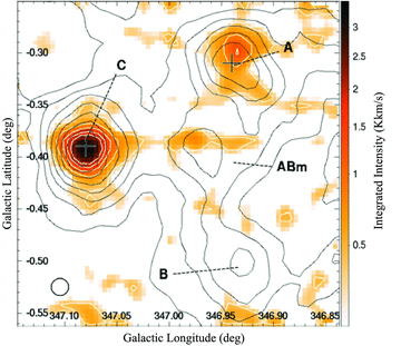
Mopra CS(J= 1–0) integrated-intensity image (vLSR=−13.5 to −9.5 km s−1) with Nanten2 CO(J= 2–1) (vLSR=−18 to 0 km s−1) contours (black) and two 8  m point sources indicated by crosses. CO(J= 2–1) contours span 5–40 K km s−1 in increments of 5 K km s−1. CS(J= 1–0) contours (white) are also shown, spanning from 0.4 to 2.0 K km s−1 in increments of 0.4 K km s−1. The beam FWHM of Mopra at 49 GHz is displayed in the bottom left-hand corner.
Figs 3–9 show CS(J= 1–0) spectra from pointed observations towards Cores A, B, C and D, and Point ABm. Corresponding CO(J= 1–0) spectra (Moriguchi et al. 2005) are also shown in these figures, but the CO beam FWHM of ∼180 arcsec, corresponding to ∼9× the 7-mm solid angle, means that neighbouring gas is probably included in the beam average.
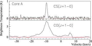
Core A: CS(J= 1–0) spectrum (top) and CO(J= 1–0) spectrum (bottom) towards Core A. The position of Core A is that displayed in Table 2.
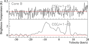
Core B: CS(J= 1–0) spectrum (top) and CO(J= 1–0) spectrum (bottom) towards Core B. The position of Core B is that displayed in Table 2.
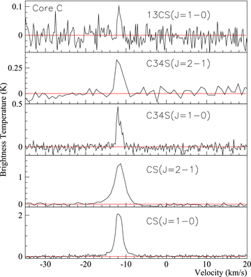
Core C: CS isotopologue spectra towards Core C. The position of Core C is that displayed in Table 2.
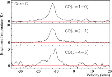
Core C: various CO spectra towards Core C (Fukui et al. 2003; Moriguchi et al. 2005; Fukui et al. 2008; Sano et al. 2010). The position of Core C is that displayed in Table 2.
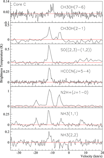
Core C: various spectra towards Core C. The position of Core C is that displayed in Table 2.
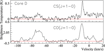
Core D: CS(J= 1–0) spectrum (top) and CO(J= 1–0) spectrum (bottom) towards Core D. CS(J= 1–0) emission has been box-car-smoothed over six channels. The position of Core D is that displayed in Table 2.
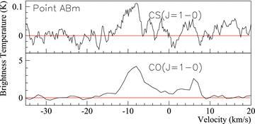
Point ABm: CS(J= 1–0) spectrum (top) and CO(J= 1–0) spectrum (bottom) towards Point ABm. CS(J= 1–0) emission has been box-car-smoothed over six channels. The position of Point ABm is that displayed in Table 2.
Core A exhibits symmetric narrow line CS(J= 1–0) emission, of ΔvFWHM∼ 1.25 km s−1, suggesting that the inner, dense core is not under the influence of an exterior shock. Fig. 1(b) shows that the forward shock is coincident with the outskirts of Core A such that the inner CS(J= 1–0)-emitting region probably remains unaffected by the RX J1713.7−3946 shock, consistent with our observations.
Core C displays the strongest CS(J= 1–0) emission of this survey, implying that this region probably harbours the largest mass dense core. CO(J= 4–3) observations by Sano et al. (2010) suggested that Core C contains a bipolar outflow, but we find no obvious asymmetries in the CS(J= 1–0) emission line profile or map data. We do, however find a significant difference between the red and blueshifted sides of CS(J= 2–1) emission. For deep switched pointing spectra, fitted Gaussians were subtracted from the observed spectra of CS(J= 1–0, J= 2–1) emission, and the resultant spectra were integrated over velocity ranges chosen, by eye, to represent red and blue-shifted line wings. Integrating CS(J= 2–1) emission over 4.1 km s−1 wide bands, 3.0 km s−1 either side of the peak emission, highlights a 2–2.5σ intensity difference between red- and blueshifted sides, possibly tracing manifestations of the Core C bipolar outflow seen by Sano et al. (2010) in CO emission lines. No significant asymmetry (<1σ) is viewed in CS(J= 1–0) emission spectra, while in the plane of the sky, there is no significant offset between the red- and blueshifted CS(J= 1–0) emission peaks.
In the northern part of the remnant, Core D exhibits a CS(J= 1–0) emission line with a FWHM of 2.5 ± 0.3 km s−1, slightly larger than that for Cores A and C. This might be expected given that Core D harbours an IRAS point source more luminous than that of the other cores associated with RX J1713.7−3946 (Moriguchi et al. 2005), but Core D also lies on the northern shock front, another possible source of disruption. Towards Core D, a second peak at vLSR=∼−70 km s−1 (∼6 kpc) was detected. This Norma-arm gas, initially suggested by Slane et al. (1999) to be associated with RX J1713.7−3946, is probably unassociated, given the preference for a 1 kpc distance (see Section 1).
Deep observations on a location at the midpoint of Cores A and B, Point ABm, revealed weak and moderately broad CS(J= 1–0) emission of FWHM, ΔvFWHM= 4 ± 1, possibly indicating the existence of a passing shock, as there is no evidence to support star-formation towards this location. This scenario is qualitatively supported by the positional coincidence of Point ABm with the western shock-front (see Section 1), but the low signal-to-noise ratio means that any conclusions drawn from this are low confidence. Alternatively, small-scale unresolved clumps (perhaps from star formation) may be responsible for the detection.
3.2 Other molecular species
No emission from the shock tracer, SiO, was seen in maps or pointed observations. The RX J1713.7−3946 shock-front likely exceeds 1000 km s−1, which may dissociate molecules in the region, but also initiate non-dissociative subsidiary shocks in dense gas, as discussed by Uchiyama et al. (2010) for older SNRs. Given the existence of dense gas in the region, as indicated by this study, one might indeed expect such secondary shocks if the gas lies within the SNR shell. In such scenarios, it may be expected that Si is sputtered from dust grains, increasing the gas-phase abundance of SiO in the post-shock region (see for example Schilke et al. (1997)). As we do not detect SiO towards this region of RX J1713.7-3946, we conclude that, if the SN shock is indeed interacting with the surveyed gas as indicated by high energy emissions (see Section 1), it has not produced SiO at detectable levels.
Detections of the organic molecules HC3N and CH3OH were recorded from Core C and HC3N from Core A. CH3OH is believed to be the product of grain-surface reactions. Weak emission from this molecule suggests that conditions within the core are capable of evaporating a significant amount of the ice mantles of grains into gas phase.
N2H+ and NH3 were both detected inside Core C. NH3 is generally thought to be a tracer of cool, quiescent gas, as its main reaction pathways do not require high temperatures (Le Bourlot 1991). The main reaction pathway of N2H+ is through molecular nitrogen interacting with H (Hotzel, Harjul & Walmsley 2004), so N2H+ can be thought as a tracer of molecular nitrogen.
4 MILLIMETRE EMISSION-LINE ANALYSES
Local thermodynamic equilibrium (LTE) analyses using NH3(1,1), NH3(2,2), CS(J= 1–0), CS(J= 2–1) and N2H+(J= 1–0) were applied to estimate gas parameters. For brevity, the mathematics of our molecular emission analyses is not presented here, but in Appendix B. Optical depths were found by taking intensity ratios of emission line pairs. Rotational (or excitation in the case of N2H+) temperatures could then be estimated from LTE assumptions allowing total column densities to be calculated. The methods used are only briefly described here, but details are presented in references. After making some assumptions about core structure, masses and densities were estimated.
Gaussian functions were fitted to all emission lines using a χ2 minimization method. Lines with visible hyperfine structure (NH3 and N2H+) had each ‘satellite’ line constrained to be a fixed distance (in vLSR space) from the ‘main’ line. In addition to this, for simplicity, all NH3(1,1) emission lines were assumed to have equal FWHM.
4.1 Optical depth
The NH3(1,1) inversion transition has five distinctly resolvable peaks and the N2H+(J= 1–0) rotational transition has three (further splitting is present in both molecular transitions, but remain unresolved due to line overlap). The relative strengths of these lines (increasing in velocity space) are [0.22, 0.28, 1, 0.28, 0.22] for NH3(1,1) (Ho & Townes 1983) and [0.2, 1, 0.6] for N2H+(J= 1–0) (Womack, Ziurys & Wychoff 1992). Here, we refer to the centre lines as ‘main’ lines and all others as ‘satellite’ lines.
To estimate optical depths, τ, of NH3(1,1) and N2H+(J= 1–0), any deviations from the aforementioned relative line strengths of main and satellite emission peaks were assumed to be due to optical depth effects, allowing the use of the standard analysis presented in Barrett, Ho & Myers (1977). Note that the optical depths quoted for these two molecular transitions are those of the central emission lines, which in both cases have unresolved structure.
By assuming abundance ratios between CS and rarer isotopologue partners, C34S and 13CS, a similar method can be used to estimate the optical depth of CS emission lines. Values of 22.5 and 75 were assumed for the abundance ratios [CS]/[C34S] and [CS]/[13CS], respectively. CS emission without detected isotopologue pairs were approximated as being optically thin.
Where multiple optical depth values were calculated (4 for NH3(1,1), 2 for N2H+(J= 1–0), 3 for CS(J= 1–0,2–1), respectively), an average was taken, weighting by the inverse of the optical depth variance.
4.2 Temperature and column density
Upper-state column densities, NU, for NH3(1,1), N2H+(J= 1–0) and CS(J= 1–0, J= 2–1) were calculated via equation (9) of Goldsmith & Langer (1999).
NH3
The LTE analysis outlined in Ho & Townes (1983) and summarized in Ungerechts, Winnewisser & Walmsley (1986) was used to find rotational temperature, Trot, and total column density, Ntot, of NH3 from the NH3(1,1) and NH3(2,2) emission lines. Kinetic temperature, Tkin, was calculated from an approximation presented in Tafalla et al. (2004).
N2H+
Given the smaller beam FWHM of the 3-mm observations with Mopra (36 arcsec < 0.2 pc at 1 kpc), a filled-beam assumption for the measured N2H+(J= 1–0) lines was used to estimate the excitation temperature, Tex, in order to find the total column density assuming an approximation of a linear, rigid rotator in LTE (Hotzel et al. 2004).
CS
Because of the small separation in energy (∼4.7 K), where both CS J= 1 and J= 2 column densities were calculated, a weighted average was taken and assumed to represent the CS(J= 1) column density (after a beam-dilution correction, see Section 4.3). Where possible, an NH3-derived temperature would be assumed, otherwise a temperature of 10 K was assumed and applied in an LTE approximation to calculate the total CS column density.
4.3 Beam dilution
4.4 LTE mass and density
LTE masses, MLTE, were calculated assuming a spherical, homogeneous core of radius, R, composed of molecular hydrogen. Average abundances with respect to H2 for CS, N2H+ and NH3 were assumed to be 1 × 10⁻⁹ (Frerking et al. 1980), 5 × 10⁻¹⁰ (Pirogov et al. 2003) and 2 × 10⁻⁸ (Stahler & Palla 2005), respectively.
4.5 Virial mass
As the virial mass is not always consistent with LTE mass, the molecular abundances that give an LTE mass equal to that of the virial mass was calculated in each case.
5 CORE PARAMETERS
The critical density of the J= 1–0 transition of CS is ∼8 × 104 cm−3, implying that the density of regions traced by this emission, in this case, Cores A, C and D, is probably distributed around this value. Cores A, C and D are coincident with infrared sources (Moriguchi et al. 2005), so the detection of CS(J= 1–0) emission from these regions supports the notion that these cores harbour dense warm gas.
5.1 Core C
The 3, 7 and 12 mm observations on Core C revealed emission from six different molecular species (see Table 2). Using three of these molecular species, detailed analyses were performed. Results are displayed in Table 3, and discussed in the following subsections.
Core C parameters derived from three different molecular species assuming a core radius 0.12 pc. Optical depth, rotational temperature, kinetic temperature, molecular column density, H2 column density, LTE mass, LTE density, virial mass and molecular abundance are denoted by τ, Trot, Tkin, NX,  , MLTE, nH, Mvir and χvir. Statistical errors (rounded to the nearest significant figure) for all variables independent of virial equilibrium assumptions are shown. Systematic errors are not displayed, but are discussed in the text.
| Emission lines | τ a | Trot (K) | NX b, c (×1013 cm−2) |  (×1022 cm−2) (×1022 cm−2) | MLTE b, c, d (M⊙) | nH b, c, d (×105 cm−3) | Mvir b (M⊙) | χvir a, b, c [X]/[H2] |
| NH3(1,1) | 1.81 ± 0.51 | 21 ± 6e | 210 ± 40 | 11 ± 2 | 80 ± 10 | 3 ± 0.5 | 30 | 5 × 10⁻⁸ |
| NH3(2,2) | 0.40 ± 0.08 | |||||||
| N2H+(J= 1–0) | 1.06 ± 0.23 | 4.5 ± 0.2b, f | 5 ± 1 | 11 ± 3 | 80 ± 20 | 3 ± 1 | 70 | 5 × 10⁻¹⁰ |
| CS(J= 1–0) | 2.71 ± 0.29 | 5.5 ± 0.4g | 55 ± 4 | 40 ± 3 | 2 ± 1 | 30h | 1 × 10⁻⁹ h | |
| CS(J= 2–1) | 50h | 7 × 10⁻¹⁰ h |
| Emission lines | τ a | Trot (K) | NX b, c (×1013 cm−2) | (×1022 cm−2) | MLTE b, c, d (M⊙) | nH b, c, d (×105 cm−3) | Mvir b (M⊙) | χvir a, b, c [X]/[H2] |
| NH3(1,1) | 1.81 ± 0.51 | 21 ± 6e | 210 ± 40 | 11 ± 2 | 80 ± 10 | 3 ± 0.5 | 30 | 5 × 10⁻⁸ |
| NH3(2,2) | 0.40 ± 0.08 | |||||||
| N2H+(J= 1–0) | 1.06 ± 0.23 | 4.5 ± 0.2b, f | 5 ± 1 | 11 ± 3 | 80 ± 20 | 3 ± 1 | 70 | 5 × 10⁻¹⁰ |
| CS(J= 1–0) | 2.71 ± 0.29 | 5.5 ± 0.4g | 55 ± 4 | 40 ± 3 | 2 ± 1 | 30h | 1 × 10⁻⁹ h | |
| CS(J= 2–1) | 50h | 7 × 10⁻¹⁰ h |
aEqual excitation temperature assumption; bAssuming a source of radius 25 arcsec (∼0.12 pc); cLTE assumption; dAssuming abundance ratios stated in Section 4.4; eTkin= 26 ± 8; fTex; gAssuming the temperature calculated from NH3; hUsing the optically thin isotopologue C34S.
Core C parameters derived from three different molecular species assuming a core radius 0.12 pc. Optical depth, rotational temperature, kinetic temperature, molecular column density, H2 column density, LTE mass, LTE density, virial mass and molecular abundance are denoted by τ, Trot, Tkin, NX, , MLTE, nH, Mvir and χvir. Statistical errors (rounded to the nearest significant figure) for all variables independent of virial equilibrium assumptions are shown. Systematic errors are not displayed, but are discussed in the text.
| Emission lines | τ a | Trot (K) | NX b, c (×1013 cm−2) | (×1022 cm−2) | MLTE b, c, d (M⊙) | nH b, c, d (×105 cm−3) | Mvir b (M⊙) | χvir a, b, c [X]/[H2] |
| NH3(1,1) | 1.81 ± 0.51 | 21 ± 6e | 210 ± 40 | 11 ± 2 | 80 ± 10 | 3 ± 0.5 | 30 | 5 × 10⁻⁸ |
| NH3(2,2) | 0.40 ± 0.08 | |||||||
| N2H+(J= 1–0) | 1.06 ± 0.23 | 4.5 ± 0.2b, f | 5 ± 1 | 11 ± 3 | 80 ± 20 | 3 ± 1 | 70 | 5 × 10⁻¹⁰ |
| CS(J= 1–0) | 2.71 ± 0.29 | 5.5 ± 0.4g | 55 ± 4 | 40 ± 3 | 2 ± 1 | 30h | 1 × 10⁻⁹ h | |
| CS(J= 2–1) | 50h | 7 × 10⁻¹⁰ h |
aEqual excitation temperature assumption; bAssuming a source of radius 25 arcsec (∼0.12 pc); cLTE assumption; dAssuming abundance ratios stated in Section 4.4; eTkin= 26 ± 8; fTex; gAssuming the temperature calculated from NH3; hUsing the optically thin isotopologue C34S.
5.1.1 Core C size
Using CS(J= 1–0) map data, we can estimate the core size by deconvolving the intensity distribution with a Gaussian of FWHM equal to the 7-mm beam FWHM. We assume that the Core C radial density profile is well approximated by a Gaussian and assume the relation r2=s2+r′2, where r, s and r′ are the observed radius, beam half width at half-maximum (HWHM)and deconvolved radius, respectively. By extending the definition of s to be the quadrature sum of both the 7 mm HWHM (29.7 arcsec) and the Gaussian smoothing HWFM of our maps (37.5 arcsec), we obtained a dense core radius of ∼25 arcsec. Thus, we assumed a core radius of 0.12 pc (25 arcsec at a distance of 1 kpc) in our calculations, yielding correction factors, fK, of 1.3, 1.3, 2.5 and 9.1 for CS(J= 2–1), N2H+(J= 1–0), CS(J= 1–0) and NH3 lines, respectively. There is a ∼50 per cent systematic uncertainty associated with our calculated radius that propagates into LTE mass (MLTE), density ( ), virial mass (Mvir) and virial abundance (χvir). We do not account for this systematic in Table 3, but discuss it in Section A2.
5.1.2 Mass and molecular abundances
The adoption of molecular abundance ratios is probably the dominant source of systematic uncertainty. It is not uncommon for molecular abundances to vary by an order of magnitude between different Galactic regions, but given the order-of-magnitude agreement between the calculated LTE masses (40–80 M⊙), the assumed abundances are probably valid. Under the assumption that turbulent energy balances gravitational energy within Core C (which may not be valid in a core that is shock disrupted), virial masses (30–70 M⊙) for these three molecular species allowed abundances with respect to molecular hydrogen to be calculated. We saw no significant deviation in CS, N2H+ and NH3 abundance (∼1×, ∼1× and ∼2.5×, respectively).
Systematic uncertainties in beam efficiency, beam dilution and beam shape corrections are difficult to account for, but propagating published systematic error estimates leads to greater than 30 per cent systematic error in N2H+ and CS LTE mass and density estimates, but has only a ∼5 per cent effect on NH3-derived mass and density estimates, since many such effects cancel-out in the analysis.
In our CS analysis of Core C, several assumptions were made. The use of an NH3-derived temperature introduces some uncertainty, as NH3 emission may trace a region of different temperature to that of CS emission. Tafalla et al. (2004) examined the starless cores L1498 and L1517B in detail and found significant variation in CS and NH3 molecular abundances with radius. NH3 (para-NH3) abundance peaked at ∼1.4 and 1.7 × 10⁻⁸ towards the core centres and dropped to ∼5 × 10⁻⁹ at ∼0.05 pc, while CS (and C34S) abundances decreased towards the centre, with models assuming a central ∼0.05 pc hole, likely due to CS depletion on to dust grains, providing a better fit to observations than constant-abundance models. It follows that it is feasible that the region emitting in CS(J= 1–0) and CS(J= 2–1) is different to that emitting in NH3(1,1). The systematic error caused by this effect is difficult to quantify, but given the factor 2 agreement between CS and NH3-derived core mass under a ‘perfect-correspondence’ assumption, it is expected to be small.
The CS J= 1 and J= 2 states are separated by only 2.35 K and a comparison of the two emission lines to retrieve a rotational temperature would likely be dominated by uncertain systematics since the two measurements were taken with different spectrometers and were separated by 2 yr. As we expect the J= 1 and J= 2 states of CS to be roughly equally populated, the optical depths and upper-state column densities were averaged to minimize instrumental systematic uncertainties (deemed to be larger than errors introduced by the equal-population assumption).
Of course, all analyses thus far have assumed LTE, which may not be valid, as suggested by CS J= 1–0 and J= 2–1 intensities. We investigate how the calculated gas parameters may differ from a more accurate non-LTE statistical equilibrium treatment using the freely available software radex (van der Tak et al. 2007). Through radex modelling, we conclude that for a CS column density of 1 × 1014 cm−2, the molecular hydrogen density may not exceed ∼6 × 104 cm−3 at a temperature of 10 K, and may be smaller for increasing temperature. This solution would have implications for the calculated mass and abundance, being ∼75 per cent smaller and ∼3 × 10⁻⁹, respectively. We note that in order to correctly simulate the observed 13CS intensity using the gas parameters outlined above (which were consistent with CS and C34S emission), the assumed value of [CS]/[13CS] must be adjusted to ∼110. Although a limited investigation of CS isotopologue abundance is presented in Section A4, we leave a more detailed examination of this for later work.
We note that our measurements seem to trace less mass than CO(J= 1–0) observations by Moriguchi et al. (2005), who calculate a Core C mass of ∼400 M⊙. This suggests that CS(J= 1–0), NH3 and N2H+ are tracing different regions of the molecular cloud to CO, most likely a denser, inner component. The Core C radial density profile is discussed further in Section A3.
5.2 Cores A and D
Table 4 shows gas parameters derived for Cores A and D. We estimate the Core A radius to be ∼0.3 pc (60 arcsec at 1 kpc) via the method described in Section 5.1.1. Core A, being more extended than Core C, and having an infrared source possibly offset from the CS(J= 1–0) peak emission (see Section 3.1), may be composed of two smaller clumps including one emitting in infrared. These inhomogeneities may even be the result of an outflow originating from IRAS 17082−3955, but this scenario remains as speculation. As our maps do not encompass Core D, we cannot estimate its radius and assume a radius of 0.12 pc for Core D (see Section A2 for alternate radius assumptions).
CS(J= 1–0) parameters for Cores A and D assuming a kinetic temperature of 10 K. No emission from a rarer isotopologue of CS is detected for these cores, so the maximum optical depth is calculated from the 1 TRMS noise in the C34S (J= 1–0) band. We display derived values for both optically thin and thick assumptions for parameters that depend on optical depth, giving a range of solutions. Optical depth, molecular column density, H2 column density, LTE mass, LTE density, virial mass and molecular abundance are denoted by τ, NCS,  , MLTE, nH, Mvir and χvir.
| Core | τ | NCS a, b (×1012 cm−2) |  (×1021 cm−2) (×1021 cm−2) | MLTE a, b, c (M⊙) | nH a, b, c (×103 cm−3) | Mvir (M⊙) | χvir [CS]/[H2] |
| Core A | 0–0.44 | 3–4 | 3–4 | 12–15 | 3–4 | 60 | 2–3 × 10⁻¹⁰ |
| Core D | 0–4.1 | 40–170 | 40–170 | 30–120 | 100–500 | 100 | 3–10 × 10−10 |
| Core | τ | NCS a, b (×1012 cm−2) | (×1021 cm−2) | MLTE a, b, c (M⊙) | nH a, b, c (×103 cm−3) | Mvir (M⊙) | χvir [CS]/[H2] |
| Core A | 0–0.44 | 3–4 | 3–4 | 12–15 | 3–4 | 60 | 2–3 × 10⁻¹⁰ |
| Core D | 0–4.1 | 40–170 | 40–170 | 30–120 | 100–500 | 100 | 3–10 × 10−10 |
aAssumed rotational temperature of 10 K.
bCorrected for beam dilution assuming a source of radius of 60 arcsec (∼0.30 pc) for Core A and 25 arcsec (∼0.12 pc) for Core D.
cAssuming abundance ratios stated in Section 4.4.
CS(J= 1–0) parameters for Cores A and D assuming a kinetic temperature of 10 K. No emission from a rarer isotopologue of CS is detected for these cores, so the maximum optical depth is calculated from the 1 TRMS noise in the C34S (J= 1–0) band. We display derived values for both optically thin and thick assumptions for parameters that depend on optical depth, giving a range of solutions. Optical depth, molecular column density, H2 column density, LTE mass, LTE density, virial mass and molecular abundance are denoted by τ, NCS, , MLTE, nH, Mvir and χvir.
| Core | τ | NCS a, b (×1012 cm−2) | (×1021 cm−2) | MLTE a, b, c (M⊙) | nH a, b, c (×103 cm−3) | Mvir (M⊙) | χvir [CS]/[H2] |
| Core A | 0–0.44 | 3–4 | 3–4 | 12–15 | 3–4 | 60 | 2–3 × 10⁻¹⁰ |
| Core D | 0–4.1 | 40–170 | 40–170 | 30–120 | 100–500 | 100 | 3–10 × 10−10 |
| Core | τ | NCS a, b (×1012 cm−2) | (×1021 cm−2) | MLTE a, b, c (M⊙) | nH a, b, c (×103 cm−3) | Mvir (M⊙) | χvir [CS]/[H2] |
| Core A | 0–0.44 | 3–4 | 3–4 | 12–15 | 3–4 | 60 | 2–3 × 10⁻¹⁰ |
| Core D | 0–4.1 | 40–170 | 40–170 | 30–120 | 100–500 | 100 | 3–10 × 10−10 |
aAssumed rotational temperature of 10 K.
bCorrected for beam dilution assuming a source of radius of 60 arcsec (∼0.30 pc) for Core A and 25 arcsec (∼0.12 pc) for Core D.
cAssuming abundance ratios stated in Section 4.4.
Given our assumptions, LTE and viral mass solutions for Core A and D range from 12 to 120 M⊙. We calculate CS abundances a factor of 0.2 to 1 of that assumed, and, like in Core C, we note that CS(J= 1–0) seems to trace less of the total mass than CO(J= 1–0). Core A and D CO-derived masses are ∼700 and ∼300 M⊙, respectively (Moriguchi et al. 2005). Similar to Core C, CS likely traces the denser, inner components of Cores A and D.
6 HIGH-ENERGY PARTICLE PROPAGATION INTO DENSE CORES
In the context of understanding the nature of the TeV gamma-ray emission from SNRs, of considerable interest is the energy-dependent propagation of high-energy protons (CRs) and electrons into dense cores, which may lead to characteristic gamma-ray spectra from GeV to TeV energies. This effect could offer a new way to identify the parent particles (hadronic versus leptonic) responsible for gamma-ray emission, provided such cores can be spatially resolved in gamma-rays. Gabici et al. (2007) investigated the propagation of CR protons into molecular clouds and found that in some models, suppressed diffusion of low-energy CRs resulted in a gamma-ray spectrum towards the cloud centre that is harder than that towards the cloud edges. This effect became more pronounced for more centrally condensed gas distributions. Similar phenomena may in fact be occurring towards the dense cores associated with RX J1713.7−3946.
We therefore investigated CR diffusion into a molecular core located adjacent to a CR accelerator. Our model is a simplistic approach that only aims to show in principle the effects that dense gas could have on the spatial distribution of CR protons of different energies, which will have knock-on effects on the gamma-ray and X-ray spectra from various parts of the core. The model configuration is based on the Core C molecular core, and its apparent location with respect to RX J1713.7−3946 as an assumed CR accelerator. CR transport in this region is expected to be in the diffusion regime, since CR (proton) gyro radii at TeV energies are expected to be <10−4 pc for typical magnetic field strengths of 10  G or more.
Our model core is placed 5 pc from the centre of RX J1713.7−3946, which has an outer shock radius growing with time to eventually reach the core, as in the situation assumed for Core C. We then calculated the propagation distance (via diffusion) of CR protons of energy, EP, from the outer shock of the SNR, towards the centre of this molecular core, applying time limits based on assumptions concerning the age of RX J1713.7−3946, and the escape time of CRs from the SNR outer shock.
The molecular core
 . If we assume the relation stated in Crutcher (1999):
 G.
G.6.1 Cosmic ray proton transport
In the hadronic scenario for gamma-ray production, CR protons diffuse from acceleration sites and collide with matter to create TeV emission. The rate of diffusion of CRs is governed by magnetic turbulence, the characteristics of which are somewhat uncertain.
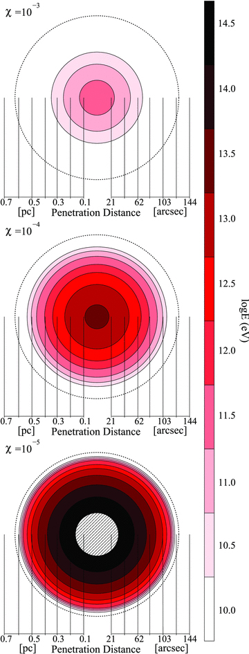
The logarithm of the minimum energy CR proton able to penetrate into different radii of our simulated core. The results, presented as 2D slices, from three different diffusion suppression coefficients χ are displayed. Note that the arcsec scale for penetration distance assumes a distance of 1 kpc. Hatching indicates a lack of CR inhabitance of CRs.
 ) and density (n≲ 1 cm−3) environment.
Escape time
Diffusion

Interactions
Diffusion suppression and results
Diffusion-suppression coefficients χ= 0.1, 0.01, 10−3, 10−4 and 10−5 were trialled for proton energies 1010, 1010.5, up to 1014 eV. This wide range of χ values were chosen to investigate the level of CR penetration with results from the smaller χ values displayed in Fig. 10.
For χ= 0.1 and 0.01, all CR energies were able (on average) to reach the inner core within the age of the system. For χ= 10−3, some energy-dependent penetration could be seen, as CRs of energies 1010 and 1010.5 eV did not reach the inner core. Energy separation became more prominent with smaller values of χ, as illustrated in Fig. 10. For χ= 10−4 and 10−5, CRs of energy 1012.5 to >1014 are now excluded from the central regions of the core. This effect would have implications for the spectrum of gamma-ray emission, with the TeV gamma-ray spectrum becoming progressively harder towards the core’s centre.
It is unclear whether such extreme cases of diffusion suppression down to χ= 10−5 required to produce these energy-dependent penetration effects on such small scales are plausible. Radio continuum measurements by Protheroe et al. (2008) when compared to the GeV gamma-ray emission have suggested upper limits for χ < 0.02 to <0.1 (dependent of the assumed magnetic field) inside the Sgr B2 molecular cloud (see also Jones et al. 2011). Suppressed CR diffusion (χ∼ 0.01–0.1) is also indicated when explaining the GeV to TeV gamma-ray spectral variation seen in the vicinity of several evolved SNRs (e.g. Gabici et al. 2010). Moreover it has been recognized that suppressed diffusion could be expected in turbulent magnetic fields likely to be found in and around shock-disrupted regions (e.g. Ormes, Ozel & Morris 1988). Overall, we regard these uncertainties in particle transport properties as motivation for investigating the effects of a wide range of diffusion suppression coefficients, as applied to our model core which may also be similarly shocked and turbulent.
From a more theoretical standpoint, the level of CR diffusion suppression that may be expected is still somewhat unclear. Yan, Lazarian & Schlickeiser (2012) recently investigated the effect of CR-induced streaming instabilities, distortions of magnetic field lines caused by the flow of CRs, on CR acceleration within SNRs. The authors expressed interest in solving for a diffusion coefficient in the region surrounding SNRs by incorporating both streaming instabilities and background turbulence. Their future work will help to constrain the level of CR diffusion suppression that can be plausibly expected inside gas associated with SNRs.
We also note that an additional CR component from the Galactic diffuse background ‘sea’ of CRs will be incident on the core. Given this is an ever-present component, the penetration of these diffuse CRs will not be limited by SNR age, but by the age of the core, and possibly by the energy loss time-scale τpp due to proton–proton collisions (equation 8). For our model core with average density n= 300 cm−3, τpp will not be the dominant loss mechanism, but will become more significant in the central region (τpp∼ 600 yr for n= 105 cm−3). The dynamical age of Core C is estimated at ∼105 yr (Moriguchi et al. 2005) which is similar to the energy loss time-scale for our averaged-density model core. For most of the χ values we consider, these time-scales are significantly larger than the time taken for CRs to diffuse into the core centre. For an example extreme case, it takes ∼5 × 10⁵ yr for a 1010 eV CR to reach the core centre for χ= 10−5, so diffuse CRs will likely penetrate the core. However, the energy density of diffuse CRs, assumed to be approximately similar to the Earth-like level of CRs, would be considerably smaller (a factor of ∼10−4) than the local CR component due to an adjacent SNR (e.g. Aharonian & Atoyan 1996), so we can therefore neglect it here.
Our core model reflects only average values of density and magnetic field as so will have limitations in comparison to a core where these quantities vary with radius. Compared to the case for a varying diffusion coefficient resulting from a radially dependent density (see equations 3 and 7), our homogenous core model may underestimate the CR penetration depth in the outer region of the core, and overestimate the penetration depth towards the inner region of the core. In future work we will consider CR propagation into a core with a radially varying diffusion coefficient based on the measured power-law radial density profile from CO measurements n(r) ∼ 105/(1 + (r/0.1 pc)2.2) cm−3 (Sano et al. 2010). This model should be three-dimensional and predict a line-of-sight view of gamma/X-ray emission morphology towards the core.
Another limitation concerns the implications of the extremely low values of diffusion suppression we have used down to χ= 10−5. For such cases, which represent highly turbulent magnetic fields, the possibility of second-order Fermi reacceleration of the CRs might apply as discussed by Dogiel & Sharov (1990). Uchiyama et al. (2010) have in fact considered this effect in accounting for the GeV to TeV gamma-ray spectra towards several evolved SNRs (W51C, W44 and IC 443) by considering the reacceleration of diffuse CRs inside clouds disturbed by a supernova shock. Such effects may occur in molecular cores associated with RX J1713.7−3946, particularly those contacted by the SNR shock but at this stage we leave this as an open question. Finally, there may be a regular (or ordered) magnetic field component, which if present may either assist or hamper the penetration of CRs depending on the strength and orientation of this field component. Such modelling is beyond the scope of this investigation, but should be considered in more detailed models.
6.2 Gamma-rays from Core C
We can expect broad-band GeV to TeV gamma-ray emission from CRs penetrating the core as they interact with core protons. The level of the gamma-ray emission will reflect the energy and spatial distribution of CRs within the core coupled to the mass of protons they interact with (see e.g. Aharonian 1991; Gabici et al. 2007). Variations in the gamma-ray spectrum will reflect the energy-dependent penetration depth of CRs, and would be a feature only resolvable in gamma-rays with an angular resolution of 1 arcmin or better according to the size of the cores. The ∼6 arcmin angular resolution offered by HESS is at present not sufficient to probe for such spectral variations.
For a wide range of diffusion suppression factors χ= 10−5 to 10−3, our simple model of Core C suggests that lower energy CRs can be prevented from reaching its centre. For the more severe values of χ= 10−4 and 10−5, the CR penetration to the core centre can be limited to CRs of TeV or greater energies, which could lead to considerable differences in the gamma-ray spectra seen towards the centre and edge of the core.
The overall gamma-ray flux expected from dense cores towards RX J1713.7−3946 has been discussed by Zirakashvili & Aharonian (2010) (see their fig. 14). They suggested an enhanced TeV hadronic component towards molecular cloud cores (with combined mass ∼1000 M⊙) may be found at a level of ∼6 × 10⁻¹² erg cm−2 s−1 for energies above ∼10 TeV, which would result from CRs of energy above ∼100 TeV entering the core, which could be the case for most levels of diffusion suppression. For these gamma-ray energies the dense-core hadronic component may reach or even exceed the SNR-wide leptonic inverse-Compton component. The >10 TeV gamma-ray flux from the central regions of Core C, which is 40–80 M⊙ based on our measurements, may therefore reach a few ×10−13 erg cm−2 s−1, possibly making it detectable by future more sensitive gamma-ray telescopes such as the Cherenkov Telescope Array (CTA; The CTA Consortium 2010). With its expected 1 arcmin or better angular resolution, CTA could also potentially probe for energy-dependent penetration of the parent CRs, by examining the flux and spectra from the inner to outer regions of the core.
6.3 Electron transport and X-ray emission towards Core C
As discussed in Section 1, two synchrotron X-ray emission peaks can be observed towards the boundary of Core C (Fig. 1b). These peaks are perhaps due to increased shock interaction with the dense gas (see Sano et al. 2010; Inoue et al. 2012) giving rise to a region of enhanced magnetic field and/or electron acceleration. The observed synchrotron X-ray emission can be produced either by electrons accelerated directly by the SNR shocks outside of Core C or, by the secondary electrons from CR proton interactions with ambient gas. In the latter case, the X-ray emission spectrum could be influenced by the energy-dependent penetration of CRs into the core and for strong CR diffusion suppression (χ≤ 10−4), one might expect an X-ray spectral hardening towards the core centre, in the same way as for gamma-rays discussed in Section 6.2.
The dense gas and high column density from Core C will also suppress the X-ray flux for energies less than ∼5 keV via photoelectric absorption. Thus some X-ray emission may actually originate from within or behind Core C. The X-ray flux decrease seen in going from the boundary of Core C to its centre is ∼95 per cent. Assuming the cross-section for photoelectric absorption by hydrogen, σν∼ 10−23 cm2 (at ∼1 keV), a flux decrease of 95 per cent corresponds to a traversed column density of NH∼ 3 × 1023 cm−2, similar to the column density towards Core C from our CS, N2H+ and NH3 observations which pertain to the core centre (see Table 3). Therefore it is possible that keV X-ray emission, either from secondary electrons produced deep within Core C from penetrating CRs or from external electrons directly accelerated outside and then entering Core C, is absorbed by gas within the core.
A potential way to discriminate between these two scenarios would be to have arcmin angular resolution imaging of >10 keV X-rays, for which photoelectric absorption is negligible. Forthcoming hard X-ray telescopes such as Astro-H (Takahashi et al. 2010) and NuSTAR (Harrison et al. 2010) are expected to have such performance. Any >10 keV X-ray emission centred on or peaking towards the centre of Core C may indicate the presence of penetrating high-energy CRs, particularly if the energy spectrum of the X-rays hardens towards the core. If this effect results from suppression of CR diffusion as discussed in Section 6.1 the same suppression effect will apply to external electrons accelerated outside the core. Strong synchrotron radiative losses on the increasing magnetic field towards the core centre may further limit the X-ray component and/or alter the spectrum from these external electrons, to the effect that X-ray emission may appear somewhat edge- or limb brightened in contrast to a more centrally peaked component from secondary electrons inside the core. For example the synchrotron cooling time  yr of electrons of energy E responsible for X-ray photons of energy ε, where
  TeV, can be compared with the diffusion time
  yr into the core with radius R= 0.62 pc. For hard X-ray photons ε∼ 10 keV and suppressed diffusion χ < 10−3, we find that tsync can become similar to or considerably less than td as B increases beyond
  G towards the centre of the core. For smaller values of χ, tsync becomes less than td for even smaller values of B.
7 SUMMARY AND CONCLUSION
We used the Mopra 22-m telescope to map in 7-mm lines a region of gas towards the western rim of the gamma-ray-emitting SNR RX J1713.7−3946, encompassing the molecular cores A, B and C (labelled by Moriguchi et al. 2005). Deep 7- and 12-mm pointed observations were also taken towards several of these regions (including Core D in the eastern rim) and we analysed archival 3-mm data towards Core C. Our goals were to investigate the extent and properties of the dense gas components towards RX J1713.7−3946 and to complement previous CO studies of the low to moderately dense gas (Fukui et al. 2003; Moriguchi et al. 2005; Fukui et al. 2008; Sano et al. 2010). The major conclusions from our observations are summarized as follows.
Detection of CS(J= 1–0) emission towards three of the four cores sampled (Cores A, C and D which have coincident infrared emission) confirming the presence of high-density (>104 cm−3) gas.
Detection of moderately broad CS(J= 1–0) emission towards a position in between Cores A, B and C (labelled Point ABm) which is towards the X-ray outer shock. This broad gas may result from the SNR shock passing through, although no shock-tracing SiO emission was observed at this position.
The LTE mass for the brightest core, Core C, was estimated using three different molecular species, with results ranging from ∼40 M⊙ from CS observations to 80 M⊙ from NH3 and N2H+ observations. The range of masses is most likely attributed to uncertainty in molecular abundances with respect to molecular hydrogen. Virial assumptions allowed molecular abundances with respect to molecular hydrogen of ∼5 × 10⁻⁸, ∼5 × 10⁻¹⁰ and ∼0.7 to 1 × 10⁻⁹ for NH3, N2H+ and CS, respectively, to be calculated for Core C. Preliminary non-LTE radex modelling suggests a factor of 2 lower density than our LTE results.
Cores A and D were found to have LTE masses of 12–15 and 30–120 M⊙, respectively, as traced by CS(J= 1–0) emission, although these values are subject to core–radius uncertainties.
The inferred column density of our CS and N2H+ measurements towards Core C could lead to considerable photoelectric absorption (∼95 per cent) of the <5 keV X-ray emission. The small-scale keV X-ray features on the border of Core C therefore might not represent the complete X-ray emission towards this core.
We investigated energy-dependent diffusion of TeV cosmic ray protons into Core C using a simple model for the core based on average values of density and magnetic field. For the cases of suppressed diffusion coefficients with factors ∼χ= 10−3 down to 10−5, lower than the Galactic average, considerable differences in the penetration depths between GeV and TeV CRs were found, with GeV CRs preferentially excluded. This effect could lead to a characteristic hardening of the TeV gamma-ray and hard X-ray emission spectrum peaking towards the core centre. Such features may be detectable and resolvable with future gamma-ray and X-ray telescopes and therefore offer a novel way to probe the level of accelerated CRs from RX J1713.7−3946 and the strength and structure of the magnetic field within the core. A more detailed diffusion model assuming a variable density and magnetic field is left for later work. We would also finally note that mapping in tracers of cosmic ray ionization such as DCO+ and HCO+ (Indriolo et al. 2010; Montmerle 2010) could be a highly valuable link between RX J1713.7−3946 and the observed gas and provide complementary information on the level of low-energy MeV to GeV CRs impacting the molecular cores.
We would like to thank Stefano Gabici and Felix Aharonian for useful discussions about the diffusion of CRs, and Malcolm Walmsley for his insightful comments. This work was supported by an Australian Research Council grant (DP0662810). The Mopra Telescope is part of the Australia Telescope and is funded by the Commonwealth of Australia for operation as a National Facility managed by the CSIRO. The University of New South Wales Mopra Spectrometer Digital Filter Bank used for these Mopra observations was provided with support from the Australian Research Council, together with the University of New South Wales, University of Sydney, Monash University and the CSIRO.
Footnotes
REFERENCES
Appendices
APPENDIX A: THE MOLECULAR CORES IN FURTHER DETAIL
A1 C![formula]() S and HC
S and HC![formula]() N emission
N emission
C34S(J= 1–0) emission can be viewed towards Core C (Fig. A1, top). This is further evidence of the existence of a dense molecular core and, with the CS(J= 1–0) spectral line, allows the calculation of the optical depth and column density. HC3N(J= 5–4) emission from Cores A and C (Fig. A1, middle and bottom) are also indicative of dense cores.
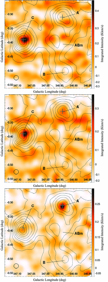
Top: C34S(J= 1–0) vLSR=−13.5 to −9.5 km s−1. Middle: HC3N(J= 5–4) vLSR=−13.5 to −9.5 km s−1. Bottom: HC3N(J= 5–4) vLSR=−11.0 to −9.0 km s−1.
A2 Scaling factors
In this investigation, the Core C radius of 0.12 pc, as calculated from CS(J= 1–0) emission, has an uncertainty of ∼50 per cent and may not necessarily be representative of core sizes traced by NH3(1,1) and N2H+(J= 1–0) emission. This radius was also assumed for Core D. We therefore provide scaling factors (Table A1) normalized to a core radius of 0.12 pc to allow parameter estimates derived from the three molecular species to be readily scaled to represent different source size assumptions. These were derived by simply calculating gas parameters for other core radius assumptions and dividing this by the result for a core radius of 0.12 pc.
Mass, M, density, nH, and abundance, χvir, scaling factors versus assumed Core C radius. Gas parameters derived from an assumed radius of 0.12 pc can be readily converted to be for other assumed core radii by multiplying the value by the appropriate correction.
| Core radius (pc) | 0.05 | 0.1 | 0.15 | 0.2 | 0.25 | 0.3 |
| M | Mass scaling factors | |||||
| LTE 12 mm | 5.7 | 1.5 | 0.68 | 0.41 | 0.28 | 0.22 |
| LTE 7 mm | 5.3 | 1.4 | 0.72 | 0.50 | 0.41 | 0.37 |
| LTE 3 mm | 3.7 | 1.2 | 0.85 | 0.76 | 0.75 | 0.74 |
| Virial | 0.42 | 0.83 | 1.25 | 1.67 | 2.08 | 2.50 |
 | Density scaling factors | |||||
| LTE 12 mm | 83 | 2.7 | 0.37 | 0.09 | 0.03 | 0.01 |
| LTE 7 mm | 77 | 2.6 | 0.39 | 0.11 | 0.05 | 0.03 |
| LTE 3 mm | 53 | 2.3 | 0.46 | 0.17 | 0.09 | 0.05 |
| χvir | Molecular abundance scaling factors | |||||
| 12 mm (NH3) | 14 | 1.8 | 0.56 | 0.25 | 0.14 | 0.09 |
| 7 mm (CS) | 13 | 1.7 | 0.59 | 0.30 | 0.20 | 0.15 |
| 3 mm (N2H+) | 8.9 | 1.5 | 0.69 | 0.47 | 0.36 | 0.30 |
| Core radius (pc) | 0.05 | 0.1 | 0.15 | 0.2 | 0.25 | 0.3 |
| M | Mass scaling factors | |||||
| LTE 12 mm | 5.7 | 1.5 | 0.68 | 0.41 | 0.28 | 0.22 |
| LTE 7 mm | 5.3 | 1.4 | 0.72 | 0.50 | 0.41 | 0.37 |
| LTE 3 mm | 3.7 | 1.2 | 0.85 | 0.76 | 0.75 | 0.74 |
| Virial | 0.42 | 0.83 | 1.25 | 1.67 | 2.08 | 2.50 |
| Density scaling factors | |||||
| LTE 12 mm | 83 | 2.7 | 0.37 | 0.09 | 0.03 | 0.01 |
| LTE 7 mm | 77 | 2.6 | 0.39 | 0.11 | 0.05 | 0.03 |
| LTE 3 mm | 53 | 2.3 | 0.46 | 0.17 | 0.09 | 0.05 |
| χvir | Molecular abundance scaling factors | |||||
| 12 mm (NH3) | 14 | 1.8 | 0.56 | 0.25 | 0.14 | 0.09 |
| 7 mm (CS) | 13 | 1.7 | 0.59 | 0.30 | 0.20 | 0.15 |
| 3 mm (N2H+) | 8.9 | 1.5 | 0.69 | 0.47 | 0.36 | 0.30 |
Mass, M, density, nH, and abundance, χvir, scaling factors versus assumed Core C radius. Gas parameters derived from an assumed radius of 0.12 pc can be readily converted to be for other assumed core radii by multiplying the value by the appropriate correction.
| Core radius (pc) | 0.05 | 0.1 | 0.15 | 0.2 | 0.25 | 0.3 |
| M | Mass scaling factors | |||||
| LTE 12 mm | 5.7 | 1.5 | 0.68 | 0.41 | 0.28 | 0.22 |
| LTE 7 mm | 5.3 | 1.4 | 0.72 | 0.50 | 0.41 | 0.37 |
| LTE 3 mm | 3.7 | 1.2 | 0.85 | 0.76 | 0.75 | 0.74 |
| Virial | 0.42 | 0.83 | 1.25 | 1.67 | 2.08 | 2.50 |
| Density scaling factors | |||||
| LTE 12 mm | 83 | 2.7 | 0.37 | 0.09 | 0.03 | 0.01 |
| LTE 7 mm | 77 | 2.6 | 0.39 | 0.11 | 0.05 | 0.03 |
| LTE 3 mm | 53 | 2.3 | 0.46 | 0.17 | 0.09 | 0.05 |
| χvir | Molecular abundance scaling factors | |||||
| 12 mm (NH3) | 14 | 1.8 | 0.56 | 0.25 | 0.14 | 0.09 |
| 7 mm (CS) | 13 | 1.7 | 0.59 | 0.30 | 0.20 | 0.15 |
| 3 mm (N2H+) | 8.9 | 1.5 | 0.69 | 0.47 | 0.36 | 0.30 |
A3 Core C radial density profile
Sano et al. (2010) used CO measurements to derive a power-law radial density profile of index −2.2 ± 0.4 (Fig. A2). Extrapolating the model to R < 0.12 pc yields a number density value of ∼2 × 104 cm−3. Our LTE results indicate a density of 2–3 × 105 cm−3 and virial densities are 1–4 × 105 cm−3, all an order of magnitude larger than that indicated by CO.
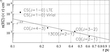
Average density within radius, as traced by CO (Sano et al. 2010) and CS (this work). A −2.2 power-law function is also displayed for comparison (not fitted). Uncertainties are not displayed and are discussed in the text.
It follows that the Core C density profile may increase beyond the CO-derived power law at smaller radii, but this discrepancy could be due to abundance uncertainties discussed in Section 5.1.2. This would not account for the discrepancy in virial-derived densities, which may simply be due to the virial assumption being invalid for Core C. If the apparent core radius varies between different molecular transitions, densities derived from different emission lines could be scaled independently (see Table A1), potentially changing estimates by an order of magnitude.
A4 CS isotopologues
A key assumption in the optical depth calculations is that of the sulphur and carbon isotope ratio values, [CS]/[C34S] ∼ [32S]/[34S] ∼ 22.5 and [CS]/[13CS] ∼ [12C]/[13C] ∼ 75, respectively. These assumptions can be investigated by comparing the emission of 13CS and C34S. The 13CS(J= 1–0)/C34S(J= 1–0) peak intensity ratio from Core C is 0.26 ± 0.06, which would appear to be consistent with the adopted abundance ratios (22.5/75 = 0.3). On the other hand, the integrated intensity ratio is 0.16 ± 0.05, somewhat inconsistent with our abundance assumptions. This is of concern as integrated intensity is more relevant than peak intensity when calculating molecular abundances. We reviewed 13CS(J= 1–0)/C34S(J= 1–0) integrated intensity ratios in published literature towards a variety of cores.
Fig. A3 presents a histogram of the ratio of integrated intensities of 13CS and C34S emission from this sample. The graph suffers from low number statistics, but it can be seen that there is a large range of recorded [13CS]/[C34S] values, and although the Core C RX J1713.7−3946 data point is at the low end of the distribution, it represents only a ∼1σ deviation from the average value of 0.55 (excluding the Sickle sources). Noteworthy in Fig. A3 are two Galactic centre sources that recorded [13CS]/[C34S] values of over 4σ from the mean. More data would be useful to compare the [13CS]/[C34S] ratio of Core C to that of other cores.
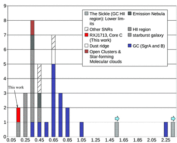
13CS/C34S integrated intensity ratios for the J= 1–0, J= 2–1 and J= 3–2 transitions. Data taken from Frerking et al. (1980), Martin et al. (2008), Martin et al. (2005) and Nicholas et al. (2011). Typical statistical error in data values is 25 per cent.
APPENDIX B: THE LTE ANALYSES IN DETAIL
B1 Ammonia analysis
B1.1 Optical depth
B1.2 Rotational and kinetic temperature
B1.3 Column density
B2 N2H+ analysis
B2.1 Optical depth

B2.2 Excitation temperature

B2.3 Column density
B3 CS
B3.1 Optical depth
B3.2 Column density
B3.3 Rotational temperature
B4 LTE mass, density and virial abundance


