


Abstract
The photospheres of about 10–20 per cent of main-sequence A- and B-type stars exhibit a wide range of chemical peculiarities, often associated with the presence of a magnetic field. It is not exactly known at which stage of stellar evolution these chemical peculiarities develop. To investigate this issue, in this paper we study the photospheric compositions of a sample of Herbig Ae and Be stars, which are considered to be the pre-main-sequence progenitors of A and B stars. We have performed a detailed abundance analysis of 20 Herbig stars (three of which have confirmed magnetic fields), and one dusty young star. We have found that half the stars in our sample show λ Boötis (λ Boo) chemical peculiarities to varying degrees, only one star shows weak Ap/Bp peculiarities and all the remaining stars are chemically normal. The incidence of λ Boo chemical peculiarities we find in Herbig stars is much higher than what is seen on the main sequence. We argue that a selective accretion model for λ Boo star formation is a natural explanation for the remarkably large number of λ Boo stars in our sample. We also find that the magnetic Herbig stars do not exhibit a range of chemical compositions remarkably different from the normal stars: one magnetic star displays λ Boo chemical peculiarities (HD 101412), one displays weak Ap/Bp peculiarities (V380 Ori A) and one (HD 190073) is chemically normal. This is completely different from what is seen on the main sequence, where all magnetic A and cool B stars show Ap/Bp chemical peculiarities, and this is consistent with the idea that the magnetic field precedes the formation of the chemical peculiarities typical of Ap and Bp stars.
1 INTRODUCTION
In main-sequence A and B stars a wide range of peculiar chemical abundances is observed. While much study has been devoted to these peculiar objects, a lot remains to be learnt about the physical processes behind these chemical peculiarities. An avenue of study that has not yet been properly investigated is to examine the chemistry in the pre-main-sequence progenitors of main-sequence peculiar stars.
Herbig Ae and Be (HAeBe) stars are pre-main-sequence A and B stars, and thus evolve into the wide range of different main-sequence A and B stars. Observationally, Herbig stars are generally identified by optical emission lines, infrared excess, and are usually associated with nebulous regions (Vieira et al. 2003). Chemically, these stars are thought to possess approximately solar abundances (Acke & Waelkens 2004), similar to most young, nearby main-sequence stars.
A small number of HAeBe stars have recently been found to have strong, globally ordered magnetic fields (Donati et al. 1997; Wade et al. 2005, 2007; Catala et al. 2007; Alecian et al. 2008a,b). The strength and morphology of these magnetic fields are very similar to those seen in the magnetic chemically peculiar Ap and Bp stars (Alecian et al. 2008a, 2009; Folsom et al. 2008), making these magnetic HAeBe stars strong candidates for the progenitors of Ap and Bp stars (Wade et al. 2005). This discovery in particular raises the question of whether any sign of chemical peculiarity can be found on the pre-main sequence.
In main-sequence A and cooler B stars, magnetic fields are always seen together with the characteristic chemical peculiarities of Ap and Bp stars (Aurière et al. 2007). Hotter magnetic B stars also usually show chemical peculiarities, such as He-weak or He-strong stars. Consequently, if magnetic HAeBe stars evolve into Ap and Bp stars, then at some point they must develop chemical peculiarities. Detecting such peculiarities on the pre-main sequence would provide new constraints on the time-scales on which, and the conditions under which, these peculiarities evolve.
A few detections of chemical peculiarities in very young stars near or on the zero-age main-sequence (ZAMS) provide tantalizing hints that chemical peculiarities may be common in magnetic HAeBe stars. Some notable cases of this are V380 Ori (Alecian et al. 2009), HD 72106 A (Folsom et al. 2008), NGC 6611 W601 (Alecian et al. 2008b) and perhaps NGC 2244−334 (Bagnulo et al. 2004) which is a very young main-sequence star. Recent modelling by Vick et al. (2011) of chemical diffusion in the presence of modest mass loss suggest it is possible for chemical peculiarities to form during the pre-main-sequence phase. Interestingly, Cowley et al. (2010) found a different form of chemical peculiarities, λ Boötis (λ Boo) peculiarities, in the Herbig Ae star HD 101412.
λ Boo stars are mostly main-sequence A stars, with strong underabundances of many metals, particularly iron peak elements. Lighter elements, specifically C, N, O, S and in some cases Na, have normal abundances, while iron peak elements are usually depleted by ∼1 dex (e.g. Venn & Lambert 1990; Andrievsky et al. 2002; Heiter 2002). This is in contrast to almost all other chemically peculiar A and B stars, which are characterized by strong overabundances of iron peak elements. λ Boo stars have not been found to have magnetic fields, unlike Ap and Bp stars (Bohlender & Landstreet 1990). λ Boo stars have a distribution of vsin i values that is the same as for normal A and B stars (e.g. Abt & Morrell 1995), unlike Ap or Am stars.
The cause of the peculiar abundances seen in λ Boo stars remains unknown, though a number of hypotheses have been suggested. The most popular hypothesis is that the peculiarities are a result of a selective accretion process (Venn & Lambert 1990; Waters, Trams & Waelkens 1992). In this scenario, gas depleted in heavier elements is accreted preferentially, building up a layer of relative underabundance in heavier elements at the surface of the star. A proposed mechanism for this suggests that heavier elements are bound into dust grains, which are then preferentially driven away from the star by its radiation, while gas, which is depleted in heavier elements as a consequence of dust formation, is more readily accreted (e.g. Andrievsky & Paunzen 2000). Thus, because of the lack of significant convective mixing in the atmospheres of A-type stars, a layer that is underabundant in heavier elements is quickly built up at the surface of the star.
A variation on this hypothesis is that the λ Boo peculiarities result from selective accretion of gas in the interstellar medium, rather than pre-existing circumstellar material (Kamp & Paunzen 2002). In this scenario the star passes through a diffuse interstellar cloud, in which heavier elements are already preferentially bound into dust grains. The star then accretes the metal-poor gas, while driving away the dust by radiation pressure.
Other hypotheses have been put forward to explore the origins of λ Boo stars. For example it has been suggested that λ Boo stars are actually spectroscopic binaries (Faraggiana & Bonifacio 2005), thus the apparent underabundances would be due to continuum emission from a secondary, but this hypothesis is largely discounted (Stütz & Paunzen 2006). Radiatively driven atomic diffusion, which is the most widely accepted mechanism for forming peculiarities in most chemically peculiar A and B stars, has been considered for λ Boo stars with the addition of mass loss (Michaud & Charland 1986). However, any turbulent or rotational mixing impedes the process sufficiently to prevent it from forming λ Boo peculiarities (Charbonneau 1993). Since λ Boo stars rotate with similar vsin i to normal A stars, they potentially can have significant rotational mixing. Thus atomic diffusion is generally considered to be insufficient to cause λ Boo peculiarities.
Numerical models of λ Boo star atmospheres including the accretion of material depleted in heavier elements, together with atomic diffusion, have been made by Turcotte & Charbonneau (1993) and Turcotte (2002). They find that those models can produce λ Boo peculiarities quickly (∼0.1 Myr) for gas accretion rates of ∼10−13 M⊙ yr−1, but the peculiarities in these models do not last long after accretion has stopped (∼1 Myr). The peculiarities in these models appear to persist despite rotational mixing (Turcotte & Charbonneau 1993), but larger surface convection zones require larger accretion rates to produce the same peculiarities (Turcotte 2002).
In order to help address the question of λ Boo star formation, and to investigate when Ap/Bp stars develop chemical peculiarities, we have analysed high-resolution spectra of 20 HAeBe stars, and one dusty young star. We have determined atmospheric parameters and performed a detailed abundance analysis for these stars, with the goal of detecting chemical peculiarities. Three of these stars have confirmed magnetic field detections, and thus may be the progenitors of Ap/Bp stars. The other 18 stars have been carefully searched for magnetic fields, but no confirmed magnetic fields have been found.
2 OBSERVATIONS
Observations for this study were obtained with the Echelle Spectropolarimetric Device for the Observation of Stars (ESPaDOnS) instrument at the Canada–France–Hawaii Telescope (CFHT). ESPaDOnS is a high-resolution échelle spectropolarimeter, providing nearly continuous wavelength coverage from 3700 to 10 500 Å at a resolution of R= 65 000. All observations were obtained in spectropolarimetric mode, which provides circularly polarized Stokes V spectra, as well as total intensity Stokes I spectra. Data reduction was performed with the libre-esprit (Donati et al. 1997) package, which is optimized for the ESPaDOnS instrument, and performs calibrations and optimal spectrum extraction.
The observations were obtained over several years, between 2004 and 2006 as part of an extended campaign investigating the presence of magnetic fields in HAeBe stars. This study is discussed as a whole by Alecian et al. (2012a), and individual results are reported by Wade et al. (2005), Catala et al. (2007), Alecian et al. (2008a), Alecian et al. (2008b), Folsom et al. (2008) and Alecian et al. (2009). The observations that were analysed for this paper are reported in Table 1. Additional observations from Alecian et al. (2012a) were used to check for variability in spectral lines. The high resolution and high signal-to-noise ratio (S/N) necessary for the detection of magnetic fields in metallic lines also makes these observations very well suited to a detailed abundance analysis, thus we have an excellent data set for our study.
List of observations for which an abundance analysis was performed. The heliocentric Julian date, total integration time and peak S/N (per 1.8 km s−1 spectral pixel) in Stokes I are presented for each observation.
| Object | HJD | Integration time (s) | Peak S/N I |
| HD 17081 | 245 3422.7286 | 480 | 878 |
| HD 31293 | 245 3423.8512 | 2400 | 471 |
| HD 31648 | 245 3423.8840 | 2400 | 334 |
| HD 36112 | 245 3421.7718 | 2400 | 239 |
| HD 68695 | 245 3423.9585 | 2400 | 112 |
| HD 139614 | 245 3422.0790 | 3600 | 222 |
| HD 141569 | 245 4167.0581 | 5400 | 877 |
| HD 142666 | 245 3424.0544 | 3600 | 288 |
| HD 144432 | 245 3423.1169 | 3200 | 312 |
| HD 163296 | 245 3607.7370 | 1200 | 538 |
| HD 169142 | 245 3606.8006 | 2000 | 394 |
| HD 176386 | 245 3607.7587 | 1600 | 479 |
| HD 179218 | 245 3608.8447 | 1600 | 532 |
| HD 244604 | 245 3607.0733 | 3600 | 276 |
| HD 245185 | 245 3421.8207 | 4800 | 146 |
| HD 278937 | 245 3422.7664 | 4800 | 167 |
| T Ori | 245 3607.1183 | 3600 | 204 |
| HD 101412 | 245 4194.9520 | 7200 | 150 |
| HD 190073 | 245 4167.1543 | 2700 | 496 |
| V380 Ori | 245 3609.0940 | 4800 | 256 |
The stars analysed in this study are only a subset of the full set of targets observed by Alecian et al. (2012a). The stars selected for our study were chosen to cover a range of Teff and vsin i values. The stars were also selected to generally have only modest amounts of emission in their optical spectra, which allows for a more complete and accurate abundance analysis. Preference was given to stars that were not clearly spectroscopic binaries, and to observations with a peak S/N over 200. Stars with a confirmed magnetic field and a Teff below 15000 K were all included (except for HD 72106 A, which was studied in detail by Folsom et al. 2008).
Observations of one star (HD 101412) were obtained from the Anglo-Australian Telescope (AAT) with the University College London Echelle Spectrograph (UCLES) together with SEMPOL polarimeter. This instrument consists of a bench mounted cross-dispersed échelle spectrograph (UCLES) fibre fed from a Cassegrain mounted polarimeter unit (SEMPOL), and is fundamentally a similar instrument to ESPaDOnS. Details of the instrument can be found in Semel, Donati & Rees (1993) and Donati et al. (1997, 2003), and the observing run that the observations of HD 101412 were obtained in is described by Marsden et al. (2011). Data reduction and optimal spectral extraction were performed with a generic version of esprit (Donati et al. 1997).
Supplemental archival observations from the Focal Reducer and Spectrograph 1 (FORS1) instrument at the Very Large Telescope (VLT) were used for examining Balmer lines in many stars, and are listed in Table 2. FORS1 is a low-resolution spectropolarimeter, which produces an observed spectrum entirely in one order. This is useful as it reduces the possibility of normalization errors across Balmer lines. The observations were obtained from the study of Wade et al. (2007), and a detailed description of the observations and data reduction techniques can be found therein. While Wade et al. (2007) focused on detecting magnetic fields, we only concern ourselves with Balmer line profile shapes.
FORS1 observations used for Balmer line fitting, obtained by Wade et al. (2007). The heliocentric Julian date, total integration time and peak S/N (per 64 km s−1 spectral pixel) in Stokes I are presented for each observation.
| Object | HJD | Integration time (s) | Peak S/N I |
| HD 17081 | 245 3331.5530 | 12 | 3800 |
| HD 31293 | 245 3331.6774 | 140 | 4050 |
| HD 31648 | 245 3331.6929 | 319 | 4225 |
| HD 36112 | 245 3331.7097 | 320 | 3725 |
| HD 68695 | 245 3332.7761 | 640 | 1950 |
| HD 141569 | 245 3062.8424 | 1295 | 5650 |
| HD 142666 | 245 3063.8535 | 2800 | 2775 |
| HD 144432 | 245 3062.8983 | 2100 | 4575 |
| HD 244604 | 245 3331.6217 | 1600 | 4150 |
| HD 245185 | 245 3331.6527 | 1600 | 3925 |
| HD 278937 | 245 3330.6795 | 1860 | 2550 |
| T Ori | 245 3332.6371 | 1440 | 1900 |
| HD 101412 | 245 3062.7977 | 1350 | 1575 |
| HD 190073 | 245 3330.5153 | 215 | 3700 |
| V380 Ori | 245 3330.7576 | 480 | 1450 |
3 FUNDAMENTAL PARAMETERS
Temperature and surface gravity were first measured by fitting Balmer lines, and then confirmed and, if possible, refined by enforcing local thermodynamic equilibrium (LTE) ionization and excitation balances in the metallic line spectra of the stars during the modelling procedure.
Balmer line fitting was performed on FORS1 spectra when available, since it is easier to normalize broad spectral features when they are recorded entirely in one spectral order. When FORS1 spectra were not available, ESPaDOnS spectra were used and careful attention was paid to the normalization of Balmer lines. Continuum points well outside the wings on both sides of a Balmer line were carefully chosen, a low-order polynomial was then fit through these points, and the polynomial was checked to ensure it varied only a small amount over the Balmer line. In the ESPaDOnS spectra, careful data reduction and the absence of instrumental artefacts produced an excellent correspondence between spectral orders in regions where the orders overlap. These overlap regions were used to evaluate and minimize errors in normalization across spectral orders. For stars with both FORS1 and ESPaDOnS spectra available the normalized Balmer lines were compared to ensure the accuracy of the normalization procedure for ESPaDOnS spectra. A good agreement between the normalized ESPaDOnS and FORS1 Balmer lines was consistently found. In all cases potential normalization errors are included in the quoted uncertainties of physical parameters.
Careful attention was paid to avoid contamination of the Balmer lines by emission. In our observations the cores of most Balmer lines were partially infilled by emission. Hα was often heavily contaminated by emission, and in many stars was avoided entirely. Despite this, the wings of Hγ and Hδ generally remain free from emission. The wavelength range of possible contamination in the higher Balmer lines can usually be assessed by the more prominent emission in Hα. As a consequence of these complications, the fitting procedure was performed by hand and rather conservative uncertainties were adopted. Synthetic Balmer lines were computed from atlas9 (Kurucz 1993) model atmospheres using solar chemical abundances.
Problematically, for many of our stars there is a substantial degeneracy in effective temperature and surface gravity when fitting only the wings of Balmer lines. As a result there is a large covariance between Teff and log g, and our uncertainties often represent long ellipses in the two-dimensional parameter space. Typically these degenerate regions have a slope of +250 K in Teff for +0.1 dex in log g, though the slope generally becomes steeper towards hotter temperatures.
When good quality fits to the observations were obtainable, fitting of Teff and log g for the metallic spectra was included in our determination. The fitting procedure is described in Section 4. This method relies on the ionization and excitation balance in the star assuming LTE, but a number of potential problems can occur. Lines with any emission infilling must be avoided. Poor quality atomic data, undiagnosed line blends and non-LTE effects may also be problematic. This also requires lines with a wide range of excitation energies and multiple ionization states. Consequently, this technique could not successfully be applied to all stars in our sample. In a number of cases the excitation potential could not provide a useful constraint, but the ionization potential was still useful. In these cases the constraint provided by Balmer line fits, combined with the ionization balance could still provide fairly precise Teff and log g values.
In order to place the stars of our sample on the H–R diagram, we needed to determine accurate luminosities. Photometric Johnson V magnitudes and B−V colours were derived from the HipparcosV magnitudes using the conversion from ESA (1997). For stars without Hipparcos observations, Johnson magnitudes and colours were taken from Vieira et al. (2003), Herbst & Shevchenko (1999) and de Winter et al. (2001). These magnitudes and colours are consistent with those used by Alecian et al. (2012a).
Distance was derived using Hipparcos parallaxes, when available, from the new reduction by van Leeuwen (2007). When no parallax was available, the star was associated with an OB association or star-forming region, and a literature distance to that was taken. Associations were taken from Alecian et al. (2012a), which agree with Vieira et al. (2003). Uncertainties for these distances were taken to be the spatial extent of the associations, which were estimated from their angular size on the sky, assuming the associations are approximately spherical. For HD 169142 no association could reliably be made, and thus a literature photometric distance from Sylvester et al. (1996) was used, and generous uncertainties were assumed. Literature sources for individual distances, along with the distances themselves, can be found in Table 3.
Fundamental parameters derived for the stars in this study. τ is the fractional pre-main-sequence age. The ‘Magnetic’ column lists which stars have confirmed magnetic field detections (M), and which stars we consider to be non-magnetic (N). The references for distances are the following: avan Leeuwen (2007, Hipparcos ); bde Zeeuw et al. (1999); cSylvester et al. (1996); dBrown, de Geus & de Zeeuw (1994); eDolan & Mathieu (2001); fVieira et al. (2003). The luminosity for HD 190073 was taken from Catala et al. (2007) (indicated by *).
| ID | Teff(K) | log g | Distance (pc) | log (L/L⊙) | M/M⊙ | R/R⊙ | Age (Myr) | τ | Magnetic |
| HD 17081 | 12 900 ± 400 | 3.8 ± 0.2 | 120 ± 3a | 2.67 ± 0.04 | 4.4 ± 0.2 | 4.3 ± 0.3 |  | 0.48 | N |
| HD 31293 | 9800 ± 700 | 3.9 ± 0.3 | 139 ± 19a | 1.77 ± 0.13 | 2.55 ± 0.2 | 2.7 ± 0.5 |  | 0.65 | N |
| HD 31648 | 8800 ± 190 | 4.1 ± 0.2 | 137 ± 25a | 1.27 ± 0.16 | 2.1 ± 0.25 | 1.9 ± 0.4 |  | 0.84 | N |
| HD 36112 | 8190 ± 150 | 4.1 ± 0.4 | 279 ± 70a | 1.82 ± 0.22 | 2.8 ± 0.5 | 4.0 ± 1.0 |  | 0.52 | N |
| HD 68695 | 9000 ± 300 | 4.3 ± 0.3 | 410 ± 36b | 1.34 ± 0.08 | 2.2 ± 0.15 | 1.9 ± 0.2 |  | 0.76 | N |
| HD 139614 | 7600 ± 300 | 3.9 ± 0.3 | 147 ± 37b | 0.88 ± 0.22 | 1.7 ± 0.1 | 1.6 ± 0.4 |  | 0.82 | N |
| HD 141569 | 9800 ± 500 | 4.2 ± 0.4 | 116 ± 8a | 1.52 ± 0.07 | 2.4 ± 0.2 | 2.0 ± 0.3 |  | 0.83 | N |
| HD 142666 | 7500 ± 200 | 3.9 ± 0.3 | 145 ± 18b | 1.28 ± 0.11 | 1.95 ± 0.15 | 2.5 ± 0.3 |  | 0.63 | N |
| HD 144432 | 7400 ± 200 | 3.9 ± 0.3 | 160 ± 29a | 1.27 ± 0.16 | 1.95 ± 0.2 | 2.6 ± 0.5 |  | 0.58 | N |
| HD 163296 | 9200 ± 300 | 4.2 ± 0.3 | 119 ± 11a | 1.49 ± 0.08 | 2.3 ± 0.1 | 2.2 ± 0.2 |  | 0.71 | N |
| HD 169142 | 7500 ± 200 | 4.3 ± 0.2 | 145 ± 50c | 1.01 ± 0.30 | 1.7 ± 0.2 | 1.9 ± 0.7 |  | 0.52 | N |
| HD 176386 | 11 000 ± 400 | 4.1 ± 0.3 | 128 ± 13a | 1.79 ± 0.09 | 2.8 ± 0.2 | 2.2 ± 0.3 |  | 0.93 | N |
| HD 179218 | 9640 ± 250 | 3.9 ± 0.2 | 254 ± 38a | 2.04 ± 0.13 | 3.1 ± 0.3 | 3.7 ± 0.6 |  | 0.55 | N |
| HD 244604 | 8700 ± 220 | 4.0 ± 0.2 | 380 ± 79d | 1.83 ± 0.18 | 2.75 ± 0.4 | 3.6 ± 0.8 |  | 0.61 | N |
| HD 245185 | 9500 ± 750 | 4.0 ± 0.4 | 450 ± 50e | 1.44 ± 0.11 | 2.3 ± 0.2 | 1.9 ± 0.4 |  | 0.90 | N |
| HD 278937 | 8000 ± 250 | 4.1 ± 0.2 | 318 ± 43b | 1.04 ± 0.12 | 1.8 ± 0.1 | 1.7 ± 0.3 |  | 0.76 | N |
| T Ori | 8500 ± 300 | 4.2 ± 0.3 | 380 ± 44d | 1.67 ± 0.10 | 2.45 ± 0.15 | 3.1 ± 0.4 |  | 0.75 | N |
| HD 101412 | 8600 ± 300 | 4.0 ± 0.5 | 600 ± 100f | 1.92 ± 0.14 | 3.0 ± 0.3 | 4.2 ± 0.8 |  | 0.50 | M |
| HD 190073 | 9230 ± 260 | 3.7 ± 0.3 | >340a | 1.92 ± 0.12* | 2.9 ± 0.3 | 3.6 ± 0.5 |  | 0.62 | M |
| V380 Ori A | 12 600 ± 1000 | 4.0 ± 0.5 | 398 ± 91d | 2.66 ± 0.20 | 4.4 ± 0.7 | 4.5 ± 1.2 |  | 0.55 | M |
| V380 Ori B | 5800 ± 350 | 4.1 ± 0.3 | 398 ± 91d | 1.62 ± 0.27 | 3.3 ± 0.8 | 6.4 ± 2.2 |  | 0.0 | N |
| ID | Teff(K) | log g | Distance (pc) | log (L/L⊙) | M/M⊙ | R/R⊙ | Age (Myr) | τ | Magnetic |
| HD 17081 | 12 900 ± 400 | 3.8 ± 0.2 | 120 ± 3a | 2.67 ± 0.04 | 4.4 ± 0.2 | 4.3 ± 0.3 | | 0.48 | N |
| HD 31293 | 9800 ± 700 | 3.9 ± 0.3 | 139 ± 19a | 1.77 ± 0.13 | 2.55 ± 0.2 | 2.7 ± 0.5 | | 0.65 | N |
| HD 31648 | 8800 ± 190 | 4.1 ± 0.2 | 137 ± 25a | 1.27 ± 0.16 | 2.1 ± 0.25 | 1.9 ± 0.4 | | 0.84 | N |
| HD 36112 | 8190 ± 150 | 4.1 ± 0.4 | 279 ± 70a | 1.82 ± 0.22 | 2.8 ± 0.5 | 4.0 ± 1.0 | | 0.52 | N |
| HD 68695 | 9000 ± 300 | 4.3 ± 0.3 | 410 ± 36b | 1.34 ± 0.08 | 2.2 ± 0.15 | 1.9 ± 0.2 | | 0.76 | N |
| HD 139614 | 7600 ± 300 | 3.9 ± 0.3 | 147 ± 37b | 0.88 ± 0.22 | 1.7 ± 0.1 | 1.6 ± 0.4 | | 0.82 | N |
| HD 141569 | 9800 ± 500 | 4.2 ± 0.4 | 116 ± 8a | 1.52 ± 0.07 | 2.4 ± 0.2 | 2.0 ± 0.3 | | 0.83 | N |
| HD 142666 | 7500 ± 200 | 3.9 ± 0.3 | 145 ± 18b | 1.28 ± 0.11 | 1.95 ± 0.15 | 2.5 ± 0.3 | | 0.63 | N |
| HD 144432 | 7400 ± 200 | 3.9 ± 0.3 | 160 ± 29a | 1.27 ± 0.16 | 1.95 ± 0.2 | 2.6 ± 0.5 | | 0.58 | N |
| HD 163296 | 9200 ± 300 | 4.2 ± 0.3 | 119 ± 11a | 1.49 ± 0.08 | 2.3 ± 0.1 | 2.2 ± 0.2 | | 0.71 | N |
| HD 169142 | 7500 ± 200 | 4.3 ± 0.2 | 145 ± 50c | 1.01 ± 0.30 | 1.7 ± 0.2 | 1.9 ± 0.7 | | 0.52 | N |
| HD 176386 | 11 000 ± 400 | 4.1 ± 0.3 | 128 ± 13a | 1.79 ± 0.09 | 2.8 ± 0.2 | 2.2 ± 0.3 | | 0.93 | N |
| HD 179218 | 9640 ± 250 | 3.9 ± 0.2 | 254 ± 38a | 2.04 ± 0.13 | 3.1 ± 0.3 | 3.7 ± 0.6 | | 0.55 | N |
| HD 244604 | 8700 ± 220 | 4.0 ± 0.2 | 380 ± 79d | 1.83 ± 0.18 | 2.75 ± 0.4 | 3.6 ± 0.8 | | 0.61 | N |
| HD 245185 | 9500 ± 750 | 4.0 ± 0.4 | 450 ± 50e | 1.44 ± 0.11 | 2.3 ± 0.2 | 1.9 ± 0.4 | | 0.90 | N |
| HD 278937 | 8000 ± 250 | 4.1 ± 0.2 | 318 ± 43b | 1.04 ± 0.12 | 1.8 ± 0.1 | 1.7 ± 0.3 | | 0.76 | N |
| T Ori | 8500 ± 300 | 4.2 ± 0.3 | 380 ± 44d | 1.67 ± 0.10 | 2.45 ± 0.15 | 3.1 ± 0.4 | | 0.75 | N |
| HD 101412 | 8600 ± 300 | 4.0 ± 0.5 | 600 ± 100f | 1.92 ± 0.14 | 3.0 ± 0.3 | 4.2 ± 0.8 | | 0.50 | M |
| HD 190073 | 9230 ± 260 | 3.7 ± 0.3 | >340a | 1.92 ± 0.12* | 2.9 ± 0.3 | 3.6 ± 0.5 | | 0.62 | M |
| V380 Ori A | 12 600 ± 1000 | 4.0 ± 0.5 | 398 ± 91d | 2.66 ± 0.20 | 4.4 ± 0.7 | 4.5 ± 1.2 | | 0.55 | M |
| V380 Ori B | 5800 ± 350 | 4.1 ± 0.3 | 398 ± 91d | 1.62 ± 0.27 | 3.3 ± 0.8 | 6.4 ± 2.2 | | 0.0 | N |
Fundamental parameters derived for the stars in this study. τ is the fractional pre-main-sequence age. The ‘Magnetic’ column lists which stars have confirmed magnetic field detections (M), and which stars we consider to be non-magnetic (N). The references for distances are the following: avan Leeuwen (2007, Hipparcos ); bde Zeeuw et al. (1999); cSylvester et al. (1996); dBrown, de Geus & de Zeeuw (1994); eDolan & Mathieu (2001); fVieira et al. (2003). The luminosity for HD 190073 was taken from Catala et al. (2007) (indicated by *).
| ID | Teff(K) | log g | Distance (pc) | log (L/L⊙) | M/M⊙ | R/R⊙ | Age (Myr) | τ | Magnetic |
| HD 17081 | 12 900 ± 400 | 3.8 ± 0.2 | 120 ± 3a | 2.67 ± 0.04 | 4.4 ± 0.2 | 4.3 ± 0.3 | | 0.48 | N |
| HD 31293 | 9800 ± 700 | 3.9 ± 0.3 | 139 ± 19a | 1.77 ± 0.13 | 2.55 ± 0.2 | 2.7 ± 0.5 | | 0.65 | N |
| HD 31648 | 8800 ± 190 | 4.1 ± 0.2 | 137 ± 25a | 1.27 ± 0.16 | 2.1 ± 0.25 | 1.9 ± 0.4 | | 0.84 | N |
| HD 36112 | 8190 ± 150 | 4.1 ± 0.4 | 279 ± 70a | 1.82 ± 0.22 | 2.8 ± 0.5 | 4.0 ± 1.0 | | 0.52 | N |
| HD 68695 | 9000 ± 300 | 4.3 ± 0.3 | 410 ± 36b | 1.34 ± 0.08 | 2.2 ± 0.15 | 1.9 ± 0.2 | | 0.76 | N |
| HD 139614 | 7600 ± 300 | 3.9 ± 0.3 | 147 ± 37b | 0.88 ± 0.22 | 1.7 ± 0.1 | 1.6 ± 0.4 | | 0.82 | N |
| HD 141569 | 9800 ± 500 | 4.2 ± 0.4 | 116 ± 8a | 1.52 ± 0.07 | 2.4 ± 0.2 | 2.0 ± 0.3 | | 0.83 | N |
| HD 142666 | 7500 ± 200 | 3.9 ± 0.3 | 145 ± 18b | 1.28 ± 0.11 | 1.95 ± 0.15 | 2.5 ± 0.3 | | 0.63 | N |
| HD 144432 | 7400 ± 200 | 3.9 ± 0.3 | 160 ± 29a | 1.27 ± 0.16 | 1.95 ± 0.2 | 2.6 ± 0.5 | | 0.58 | N |
| HD 163296 | 9200 ± 300 | 4.2 ± 0.3 | 119 ± 11a | 1.49 ± 0.08 | 2.3 ± 0.1 | 2.2 ± 0.2 | | 0.71 | N |
| HD 169142 | 7500 ± 200 | 4.3 ± 0.2 | 145 ± 50c | 1.01 ± 0.30 | 1.7 ± 0.2 | 1.9 ± 0.7 | | 0.52 | N |
| HD 176386 | 11 000 ± 400 | 4.1 ± 0.3 | 128 ± 13a | 1.79 ± 0.09 | 2.8 ± 0.2 | 2.2 ± 0.3 | | 0.93 | N |
| HD 179218 | 9640 ± 250 | 3.9 ± 0.2 | 254 ± 38a | 2.04 ± 0.13 | 3.1 ± 0.3 | 3.7 ± 0.6 | | 0.55 | N |
| HD 244604 | 8700 ± 220 | 4.0 ± 0.2 | 380 ± 79d | 1.83 ± 0.18 | 2.75 ± 0.4 | 3.6 ± 0.8 | | 0.61 | N |
| HD 245185 | 9500 ± 750 | 4.0 ± 0.4 | 450 ± 50e | 1.44 ± 0.11 | 2.3 ± 0.2 | 1.9 ± 0.4 | | 0.90 | N |
| HD 278937 | 8000 ± 250 | 4.1 ± 0.2 | 318 ± 43b | 1.04 ± 0.12 | 1.8 ± 0.1 | 1.7 ± 0.3 | | 0.76 | N |
| T Ori | 8500 ± 300 | 4.2 ± 0.3 | 380 ± 44d | 1.67 ± 0.10 | 2.45 ± 0.15 | 3.1 ± 0.4 | | 0.75 | N |
| HD 101412 | 8600 ± 300 | 4.0 ± 0.5 | 600 ± 100f | 1.92 ± 0.14 | 3.0 ± 0.3 | 4.2 ± 0.8 | | 0.50 | M |
| HD 190073 | 9230 ± 260 | 3.7 ± 0.3 | >340a | 1.92 ± 0.12* | 2.9 ± 0.3 | 3.6 ± 0.5 | | 0.62 | M |
| V380 Ori A | 12 600 ± 1000 | 4.0 ± 0.5 | 398 ± 91d | 2.66 ± 0.20 | 4.4 ± 0.7 | 4.5 ± 1.2 | | 0.55 | M |
| V380 Ori B | 5800 ± 350 | 4.1 ± 0.3 | 398 ± 91d | 1.62 ± 0.27 | 3.3 ± 0.8 | 6.4 ± 2.2 | | 0.0 | N |
Using these distances, bolometric luminosities were calculated. E(B−V) was calculated using the intrinsic colours of Kenyon & Hartmann (1995), and total extinction was calculated using an RV of 5, as suggested for HAeBe stars by Hernández et al. (2004). The bolometric correction of Balona (1994) was used.
Using our luminosities and temperatures, we placed the stars on the H–R diagram, as shown in Fig. 1. Pre-main-sequence evolutionary tracks and isochrones were calculated with the cesam (Morel 1997) evolutionary code, assuming solar metallicities. The birthline, the locus of points on the H–R diagram where a star becomes optically visible, was taken from Palla & Stahler (1993), for an accretion rate of 10−5 M⊙ yr−1. By comparison to these evolutionary tracks and isochrones, we determined stellar masses, and ages with respect to the birthline. These values, along with fractional pre-main-sequence ages (τ) and radii, are presented in Table 3. The uncertainties on mass and age for a star were based on the range of evolutionary tracks and isochrones that intersect the ellipse on the H–R diagram described by the uncertainties in the star’s luminosity and Teff. Note that the choice of a birthline may introduce a further systematic uncertainty into our ages. For example, using the birthline of Behrend & Maeder (2001), with a mass-dependent accretion rate, would generally increase our ages by ∼0.5 Myr (but with the actual increase varying with mass). While we do not present uncertainties on τ, the values should be considered approximate.
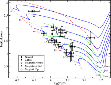
H–R diagram for the stars in this study. Evolutionary tracks (solid lines) are labelled by mass in solar masses. Isochrones (dashed lines) are labelled by age in Myr. The birthline (right dot–dashed line) for an accretion rate of 10−5 M⊙ yr−1, and the ZAMS line (left dot–dashed line) are also shown. Circles are chemically normal stars, squares are λ Boo stars and the diamond is the possible Bp star V380 Ori A. Open symbols are stars with confirmed magnetic field detections.
4 ABUNDANCE ANALYSIS
The abundance analysis and determination of vsin i and microturbulence was performed by directly fitting synthetic spectra to the observations. Model spectra were calculated using the zeeman spectrum synthesis code (Landstreet 1988; Wade et al. 2001). This code performs polarized radiative transfer under the assumption of LTE. Optimizations to the code for stars with negligible magnetic fields have been included. A Levenberg–Marquardt χ2 minimization procedure (e.g. Press et al. 1992) was used to determine best-fitting parameters.
The optimizations to the zeeman spectrum synthesis routine exploit symmetries in a non-magnetic chemically homogeneous model of a star to dramatically reduce the amount of computation required. As in the original version of zeeman, the visible disc of the star is divided into a number of surface elements. In this version it is assumed that the local emergent spectra only vary with projected radial distance from the centre of the disc of the star. Thus radiative transfer is only performed for a set of surface elements with different radial distances, and the results are reused for different angular positions, which minimize the number of times radiative transfer must be performed. The optimizations also assume the local line absorption (Voigt) and anomalous dispersion (Faraday–Voigt) profiles only vary vertically through the atmosphere, and not with position on the stellar disc, substantially reducing the number of times these profiles must be calculated. In this version of the code, limb darkening is still calculated directly, by performing radiative transfer at different radial positions on the disc of the star. Rotational broadening is also calculated directly by summing local emergent spectra that have been Doppler shifted across the disc of the star.
Detailed comparisons of the optimized code to the original version have been performed. For the same input parameters, with no magnetic field, identical spectra are produced. The original code has been checked against other spectrum synthesis codes in detail by Wade et al. (2001), with a very good agreement found. Similarly, the optimized version of zeeman has been checked against synth3 (Kochukhov 2007) and again a good agreement was found.
The Levenberg–Marquardt χ2 minimization procedure (Press et al. 1992) provides a robust and efficient routine for iteratively fitting synthetic spectra to observations. Best-fitting models from this routine have been compared to fits obtained by hand for a wide variety of stars, and good agreement between the two methods has been consistently found.
Input atomic data were taken from the Vienna Atomic Line Database (VALD; Kupka et al. 1999), using an ‘extract stellar’ request and solar chemical abundances. Updated line lists with peculiar abundances were extracted as necessary. Model atmospheres were computed using the atlas9 code (Kurucz 1993) with solar abundances. Model atmospheres were calculated on a grid in steps of 250 K in Teff and 0.5 in log g, then interpolated linearly when more precise values were desired. Interpolation on this grid of models introduces less than 1 per cent relative error to the line depths in the resulting spectrum.
Spectra were initially fit simultaneously for chemical abundances, vsin i, microturbulence and radial velocity, using the best-fitting Teff and log g determined from the Balmer lines. Then, if a good constraint could be obtained, the fits were repeated including Teff and log g as free parameters. If this produced a good fit with well constrained parameters, then these Teff and log g values were used instead of the initial Balmer line fit values. If only one of Teff and log g was well constrained from the metallic line fit, then the fit was repeated using the Balmer line value for the unconstrained parameter. We considered a parameter to be well constrained if the fitting routine reliably converged to the same value for different initial conditions, and if that value was consistent with the Balmer line profiles. The fits were generally performed on five independent regions ∼500 Å long. The approximate wavelength ranges usually were 4400–4800, 4900–5500, 5500–6000, 6000–6500 and 6600–7600 Å, and occasionally 4150–4280 Å, with significant gaps due to non-photospheric features. These windows typically contained several hundred spectral lines (the number varying greatly with wavelength and Teff), however, many of these lines are very weak and hence do not provide significant constraints on the best-fitting abundances or atmospheric parameters. The exact wavelength ranges varied between stars, due to varying regions of emission and different Balmer line widths.
Microturbulence and vsin i were determined by χ2 minimization, simultaneously with the other stellar parameters, using the entire spectral ∼500 Å window. This method relies on resolved, rotationally broadened spectral lines for constraining vsin i, and a range of both weak and strong lines for constraining microturbulence.
We verified this method of determining Teff and log g by analysing well studied stars, and comparing to literature results. In this study we have analysed π Cet, and compared our results with the very precise study by Fossati et al. (2009). Fossati et al. (2009) used photometry and spectral energy distributions, as well as Balmer lines, and excitation and ionization balances when determining their parameters. They also used different software tools to perform their modelling, thus their results are truly independent. Our results are fully consistent with theirs, as discussed in Section A1.1, which demonstrates the accuracy of our methodology.
For this method to be successful, lines contaminated by emission must be avoided. While a line entirely in emission is easily identified, lines with small amounts of emission infilling are harder to identify. When multiple observations were available, variability in the emission could be used to identify lines with emission infilling. If only one observation was available, special attention was paid to lines with low excitation potentials and large oscillator strengths, such lines being more likely to contain emission. If inconsistent fits were obtained between normal and low excitation potential lines, and no other clear explanation for the inconsistency could be found (such as an error in Teff or the atomic data), the low excitation potential lines were considered to likely contain emission and were excluded from the final fit. Additionally, the shapes of line profiles were examined and, if they could not be reproduced by the synthetic spectra, they were considered to be contaminated by a non-photospheric component. The presence of veiling in our spectra is assessed in detail in Section 6.4, and we find it is not present at a significant level.
The use of multiple spectral windows is valuable, as it allows us to take the average and standard deviation of abundances determined across the windows. The standard deviation in particular provides a reasonable estimate of the uncertainty of derived parameters. Since line-to-line abundances scatter is introduced by errors in the atomic data as well as errors in the model atmosphere, these effects are included in the standard deviation. The standard deviation may underestimate the impact of such errors, but provides a robust and easily understandable uncertainty estimate. The use of multiple spectral windows also allows us to verify the atmospheric parameters derived from metal line fits. If the parameters differ substantially from window to window, they are likely poorly constrained in some if not all windows, in which case we can rely more heavily on the parameters from Balmer line fitting.
For chemical elements with fewer than four lines providing good constraints on the abundance in any spectral window (including all cases of elements with lines in only one or two spectral windows) the uncertainties were estimated by eye rather than using a standard deviation. These uncertainties were chosen to include line-to-line scatter, uncertainties in the atmospheric parameters and potential normalization errors.
Examples of typical best-fitting synthetic spectra compared to the observed spectrum of HD 139614 in the 5000–5050 and 6100–6200 Å windows are presented in Fig. 2. Final averaged best-fitting abundances and atmospheric parameters are presented in Table 4, together with uncertainties. Elements with abundances based on less than four lines are indicated with an asterisk in the table.

Comparison of the observed spectrum (jagged line) to the best-fitting synthetic spectrum (smooth line) for HD 139614. Two independent wavelength regions are presented. Lines have been labelled by their major contributing species.
Best-fitting parameters for the stars in our sample. Chemical abundances are in units of log (NX/Ntot). Elements marked with an asterisk (*) are based on less than ∼4 useful lines and have uncertainties estimated by eye. Microturbulence is given by ξ.
| HD 17081 (π Cet) | HD 31293 (AB Aur) | HD 31648 | HD 36112 | HD 68695 | HD 139614 | HD 141569 | Solar | |
| Teff (K) | 12 900 ± 400 | 9800 ± 700 | 8800 ± 190 | 8190 ± 150 | 9000 ± 300 | 7600 ± 300 | 9800 ± 500 | |
| log g (cgs) | 3.8 ± 0.2 | 3.9 ± 0.3 | 4.1 ± 0.2 | 4.1 ± 0.4 | 4.3 ± 0.3 | 3.9 ± 0.3 | 4.2 ± 0.4 | |
| vsin i (km s−1) | 20.9 ± 1.2 | 116 ± 9 | 101.2 ± 1.7 | 57.8 ± 1.0 | 51 ± 4 | 25.6 ± 0.4 | 222 ± 7 | |
| ξ (km s−1) | 1.7 ± 1.0 | ≤4 | 3.2 ± 1.1 | 2.97 ± 0.24 | 1.3 ± 1.1 | 3.7 ± 0.4 | ≤2 | |
| He | −0.91 ± 0.14 | −1.24 ± 0.20* | −1.21 ± 0.37* | −1.11 | ||||
| C | ≤− 3.4* | −3.33 ± 0.22 | −3.67 ± 0.07 | −3.61 ± 0.16 | −3.27 ± 0.18 | −3.75 ± 0.22 | −3.63 ± 0.29 | −3.65 |
| N | −4.03 ± 0.15* | −3.9 ± 0.3* | −3.7 ± 0.3* | −4.17 ± 0.13 | −4.0 ± 0.3* | −4.26 | ||
| O | −3.16 ± 0.13 | −3.27 ± 0.20 | −3.28 ± 0.05* | −3.18 ± 0.10* | −3.17 ± 0.10 | −3.33 ± 0.10* | −3.05 ± 0.10 | −3.38 |
| Ne | −3.76 ± 0.28 | −4.20 | ||||||
| Na | −5.30 ± 0.10* | −5.72 ± 0.25* | −5.58 ± 0.15* | −6.2 ± 0.4* | −6.14 ± 0.12 | ≤− 5.2* | −5.87 | |
| Mg | −4.43 ± 0.15 | −4.89 ± 0.33 | −4.12 ± 0.13 | −4.23 ± 0.14 | −5.11 ± 0.14 | −4.74 ± 0.07 | −4.90 ± 0.11 | −4.51 |
| Al | −5.81 ± 0.17 | −5.6 ± 0.5* | −5.67 | |||||
| Si | −4.55 ± 0.14 | −4.76 ± 0.22 | −4.29 ± 0.19 | −4.58 ± 0.11 | −5.36 ± 0.15 | −5.10 ± 0.13 | −4.99 ± 0.31 | −4.53 |
| P | −6.43 ± 0.14 | −6.68 | ||||||
| S | −4.99 ± 0.08 | −4.6 ± 0.3* | −4.79 ± 0.16* | −4.6 ± 0.3* | −5.18 ± 0.15 | −4.90 | ||
| Ar | −5.6 ± 0.3* | −5.86 | ||||||
| K | −7.29 ± 0.25* | −6.96 | ||||||
| Ca | −5.7 ± 0.2* | −6.10 ± 0.17 | −5.38 ± 0.23 | −5.59 ± 0.16 | −6.47 ± 0.23 | −6.18 ± 0.16 | −6.34 ± 0.38 | −5.73 |
| Sc | −9.04 ± 0.34 | −8.72 ± 0.15 | −8.90 ± 0.26 | −9.49 ± 0.26 | −9.39 ± 0.15 | −9.18 ± 0.37 | −8.87 | |
| Ti | −7.37 ± 0.15 | −7.47 ± 0.27 | −6.82 ± 0.09 | −6.98 ± 0.20 | −7.71 ± 0.25 | −7.51 ± 0.14 | −7.74 ± 0.32 | −7.14 |
| V | −7.8 ± 0.4* | −8.4 ± 0.5* | −8.04 | |||||
| Cr | −6.57 ± 0.16 | −6.67 ± 0.27 | −6.09 ± 0.17 | −6.30 ± 0.17 | −6.98 ± 0.24 | −6.80 ± 0.11 | −7.31 ± 0.31 | −6.40 |
| Mn | −6.6 ± 0.3* | −6.59 ± 0.08 | −6.70 ± 0.16 | −6.4 ± 0.5* | −7.43 ± 0.19 | −6.65 | ||
| Fe | −4.70 ± 0.08 | −4.91 ± 0.25 | −4.47 ± 0.13 | −4.49 ± 0.14 | −5.16 ± 0.22 | −5.07 ± 0.13 | −5.25 ± 0.32 | −4.59 |
| Co | −7.12 | |||||||
| Ni | −5.85 ± 0.06 | −6.16 ± 0.27 | −5.66 ± 0.05 | −5.76 ± 0.20 | −6.25 ± 0.32 | −6.33 ± 0.14 | ≤− 6.0* | −5.81 |
| Cu | ≤− 7.5* | −8.6 ± 0.4* | −7.83 | |||||
| Zn | −7.8 ± 0.4* | −8.3 ± 0.3* | −7.44 | |||||
| Sr | −9.6 ± 0.3* | −9.4 ± 0.3* | −10.5 ± 0.5* | −9.12 | ||||
| Y | −9.57 ± 0.30 | −9.56 ± 0.17 | −10.23 ± 0.15 | −9.83 | ||||
| Zr | −9.3 ± 0.3* | −9.48 | ||||||
| Ba | −9.7 ± 0.4* | −9.56 ± 0.24* | −9.46 ± 0.29 | −10.3 ± 0.4* | −10.29 ± 0.21 | −9.2 ± 0.8* | −9.87 | |
| La | −10.91 | |||||||
| Ce | ≤− 10.5* | −10.34 | ||||||
| Nd | −10.59 | |||||||
| Eu | −11.52 | |||||||
| HD 142666 | HD 144432 | HD 163296 | HD 169142 | HD 176386 | HD 179218 | HD 244604 | Solar | |
| Teff (K) | 7500 ± 200 | 7400 ± 200 | 9200 ± 300 | 7500 ± 200 | 11 000 ± 400 | 9640 ± 250 | 8700 ± 220 | |
| log g (cgs) | 3.9 ± 0.3 | 3.9 ± 0.3 | 4.2 ± 0.3 | 4.3 ± 0.2 | 4.1 ± 0.3 | 3.9 ± 0.2 | 4.0 ± 0.2 | |
| vsin i (km s−1) | 68.0 ± 0.9 | 80.3 ± 1.0 | 122 ± 3 | 51.6 ± 0.5 | 169.0 ± 1.5 | 70 ± 4 | 101 ± 5 | |
| ξ (km s−1) | 3.55 ± 0.31 | 3.62 ± 0.23 | 1.5 ± 1.2 | 2.09 ± 0.47 | 1.7 ± 0.7 | 2.0 ± 0.5 | 1.9 ± 0.4 | |
| He | −1.17 ± 0.20* | −1.15 ± 0.15* | −1.11 | |||||
| C | −3.62 ± 0.15 | −3.79 ± 0.18 | −3.82 ± 0.25 | −3.55 ± 0.12 | −3.38 ± 0.29* | −3.45 ± 0.16 | −3.69 ± 0.17 | −3.65 |
| N | −3.9 ± 0.3* | −3.5 ± 0.4* | −4.2 ± 0.3* | −4.26 | ||||
| O | −3.18 ± 0.15* | −3.17 ± 0.10* | −3.31 ± 0.15 | −3.38 ± 0.13 | −3.20 ± 0.10* | −3.10 ± 0.13 | −3.23 ± 0.08 | −3.38 |
| Ne | −4.20 | |||||||
| Na | −5.77 ± 0.15* | −5.86 ± 0.09 | −5.6 ± 0.5* | −6.18 ± 0.08* | −5.5 ± 0.3* | −5.4 ± 0.3* | −5.87 | |
| Mg | −4.61 ± 0.06 | −4.46 ± 0.04 | −4.12 ± 0.15 | −4.89 ± 0.06 | −4.28 ± 0.15 | −4.73 ± 0.17 | −4.03 ± 0.22 | −4.51 |
| Al | −5.5 ± 0.4* | −5.5 ± 0.3* | −6.0 ± 0.4* | −5.67 | ||||
| Si | −4.91 ± 0.20 | −4.81 ± 0.24 | −4.24 ± 0.14 | −5.13 ± 0.10 | −4.44 ± 0.14 | −4.82 ± 0.22 | −4.34 ± 0.06 | −4.53 |
| P | −6.68 | |||||||
| S | −4.70 ± 0.15 | −4.82 ± 0.05 | −5.10 ± 0.12 | −4.2 ± 0.4* | −4.48 ± 0.15* | −4.90 | ||
| Ar | −5.86 | |||||||
| K | −6.96 | |||||||
| Ca | −5.98 ± 0.18 | −5.78 ± 0.15 | −5.54 ± 0.30 | −6.15 ± 0.12 | −6.27 ± 0.19* | −6.25 ± 0.38 | −5.42 ± 0.24 | −5.73 |
| Sc | −9.23 ± 0.23 | −9.09 ± 0.15 | −8.76 ± 0.08 | −9.58 ± 0.24 | −9.0 ± 0.4* | −9.40 ± 0.16 | −8.75 ± 0.24 | −8.87 |
| Ti | −7.39 ± 0.20 | −7.26 ± 0.16 | −6.92 ± 0.10 | −7.65 ± 0.10 | −7.12 ± 0.29 | −7.57 ± 0.12 | −6.81 ± 0.31 | −7.14 |
| V | −8.4 ± 0.4* | −8.3 ± 0.4* | −8.49 ± 0.16* | −8.04 | ||||
| Cr | −6.60 ± 0.21 | −6.51 ± 0.23 | −5.95 ± 0.20 | −6.98 ± 0.13 | −6.46 ± 0.21 | −6.97 ± 0.13 | −6.07 ± 0.16 | −6.40 |
| Mn | −7.08 ± 0.15 | −6.96 ± 0.15 | −7.0 ± 0.5* | −7.57 ± 0.20 | −6.91 ± 0.23 | −6.65 | ||
| Fe | −4.84 ± 0.11 | −4.70 ± 0.09 | −4.39 ± 0.15 | −5.13 ± 0.11 | −4.48 ± 0.27 | −5.03 ± 0.13 | −4.35 ± 0.24 | −4.59 |
| Co | −6.8 ± 0.4* | −7.1 ± 0.5* | ≤− 7.6* | −7.12 | ||||
| Ni | −6.16 ± 0.13 | −6.00 ± 0.15 | −5.72 ± 0.12 | −6.40 ± 0.16 | ≤− 5.9* | −6.00 ± 0.18 | −5.81 | |
| Cu | ≤− 7.7* | −8.85 ± 0.28 | −7.83 | |||||
| Zn | −7.9 ± 0.3* | −7.57 ± 0.20 | −8.71 ± 0.08* | −7.44 | ||||
| Sr | −9.56 ± 0.19* | −9.4 ± 0.3* | −9.58 ± 0.11* | −10.2 ± 0.2* | −9.12 | |||
| Y | −9.94 ± 0.22 | −9.80 ± 0.13 | −10.18 ± 0.14 | −10.0 ± 0.4* | −9.8 ± 0.4* | −9.83 | ||
| Zr | −9.36 ± 0.26* | −9.3 ± 0.4* | −9.65 ± 0.13* | −9.48 | ||||
| Ba | −9.81 ± 0.18 | −9.69 ± 0.16 | −10.0 ± 0.4* | −9.96 ± 0.21 | ≤− 9.0* | −10.4 ± 0.4* | −9.6 ± 0.2* | −9.87 |
| La | ≤− 10.8* | −11.2 ± 0.4* | −10.91 | |||||
| Ce | −10.34 | |||||||
| Nd | −10.64 ± 0.14* | −10.59 | ||||||
| Eu | −12.19 ± 0.10* | −11.52 | ||||||
| HD 245185 | HD 278937 (IP Per) | T Ori (BD -05 1329) | HD 101412 | HD 190073 | V380 Ori A | V380 Ori B | Solar | |
| Teff (K) | 9500 ± 750 | 8000 ± 250 | 8500 ± 300 | 8600 ± 300 | 9230 ± 260 | 12 600 ± 1000 | 5800 ± 350 | |
| log g (cgs) | 4.0 ± 0.4 | 4.1 ± 0.2 | 4.2 ± 0.3 | 4.0 ± 0.5 | 3.7 ± 0.3 | 4.0 ± 0.5 | 4.1 ± 0.3 | |
| vsin i (km s−1) | 136 ± 10 | 83.8 ± 4.6 | 163 ± 11 | 6.8 ± 0.4 | 8.50 ± 0.23 | 9.9 ± 1.0 | 24.7 ± 1.9 | |
| ξ (km s−1) | ≤4 | 2.0 ± 0.9 | 2.6 ± 1.1 | ≤2 | ≤2 | ≤3 | ≤2 | |
| He | −0.9 ± 0.3* | −1.4 ± 0.5* | −0.9 ± 0.3* | −0.90 ± 0.20* | −0.67 ± 0.20* | −1.11 | ||
| C | −3.72 ± 0.15 | −3.57 ± 0.17 | −3.59 ± 0.19 | −3.58 ± 0.12 | −3.72 ± 0.14 | −3.4 ± 0.4* | −3.65 | |
| N | −3.8 ± 0.4* | −4.0 ± 0.3* | −4.2 ± 0.4* | −3.60 ± 0.20* | −4.26 | |||
| O | −3.17 ± 0.17 | −3.41 ± 0.05 | −3.16 ± 0.12 | −3.12 ± 0.09 | −3.26 ± 0.11 | −3.00 ± 0.16 | −3.38 | |
| Ne | −3.8 ± 0.3* | −3.93 ± 0.36 | −4.20 | |||||
| Na | −6.3 ± 0.3* | −6.1 ± 0.3* | −5.56 ± 0.15* | −5.13 ± 0.15* | −5.95 ± 0.30* | −5.87 | ||
| Mg | −5.39 ± 0.23 | −4.91 ± 0.11 | −5.05 ± 0.23 | −4.95 ± 0.15 | −4.38 ± 0.17 | −4.19 ± 0.14 | −4.7 ± 0.7* | −4.51 |
| Al | −5.4 ± 0.5* | −5.2 ± 0.4* | −5.99 ± 0.20* | −5.58 ± 0.17* | −5.07 ± 0.21* | −5.67 | ||
| Si | −4.95 ± 0.16 | −4.97 ± 0.19 | −4.89 ± 0.20 | −5.30 ± 0.19 | −4.48 ± 0.06 | −4.11 ± 0.09 | −4.44 ± 0.26 | −4.53 |
| P | −5.86 ± 0.30* | −6.68 | ||||||
| S | −4.83 ± 0.14 | −4.1 ± 0.3* | −4.96 ± 0.12 | −4.57 ± 0.20* | −4.93 ± 0.26 | −4.90 | ||
| Ar | −5.86 | |||||||
| K | −6.96 | |||||||
| Ca | −6.12 ± 0.25 | −6.28 ± 0.18 | −6.00 ± 0.31 | −6.37 ± 0.20 | −5.61 ± 0.12 | ≤− 5.6* | −5.78 ± 0.40 | −5.73 |
| Sc | −9.6 ± 0.7* | −9.52 ± 0.21 | −9.4 ± 0.3* | −9.33 ± 0.17 | −8.85 ± 0.20 | −8.87 | ||
| Ti | −7.93 ± 0.38 | −7.81 ± 0.10 | −7.55 ± 0.17 | −7.75 ± 0.23 | −7.16 ± 0.12 | −6.78 ± 0.28 | −7.14 | |
| V | ≤− 7.5* | −8.1 ± 0.3* | −7.99 ± 0.25* | −7.50 ± 0.79 | −8.04 | |||
| Cr | −7.27 ± 0.34 | −7.04 ± 0.18 | −6.82 ± 0.07 | −6.69 ± 0.29 | −6.13 ± 0.13 | ≤− 4.8* | −5.92 ± 0.26 | −6.40 |
| Mn | −7.0 ± 0.6* | −7.3 ± 0.4* | ≤− 6.0* | −6.98 ± 0.09 | −6.54 ± 0.08 | −5.92 ± 0.16 | −5.97 ± 0.43 | −6.65 |
| Fe | −5.27 ± 0.33 | −5.12 ± 0.16 | −4.98 ± 0.10 | −5.08 ± 0.19 | −4.42 ± 0.06 | −3.92 ± 0.12 | −4.25 ± 0.16 | −4.59 |
| Co | −6.6 ± 0.6* | −7.12 | ||||||
| Ni | −6.5 ± 0.7* | −6.37 ± 0.22 | −6.13 ± 0.27 | −5.69 ± 0.17 | −5.19 ± 0.18 | −5.58 ± 0.32 | −5.81 | |
| Cu | ≤− 7.5* | −8.6 ± 0.3* | −7.4 ± 0.7* | −7.83 | ||||
| Zn | ≤− 8.0* | −7.52 ± 0.25* | −7.4 ± 0.6* | −7.44 | ||||
| Sr | −9.3 ± 0.2* | −9.12 | ||||||
| Y | −10.4 ± 0.4* | −10.12 ± 0.25 | −9.70 ± 0.20 | ≤− 8.2* | −9.83 | |||
| Zr | −9.8 ± 0.3* | −9.2 ± 0.3* | −9.48 | |||||
| Ba | −10.0 ± 0.7* | −10.2 ± 0.3* | −10.3 ± 0.3* | −10.71 ± 0.24 | −9.71 ± 0.13* | −8.89 ± 0.40 | −9.87 | |
| La | −10.91 | |||||||
| Ce | ≤− 9.6* | ≤− 8.5* | −10.34 | |||||
| Nd | −10.2 ± 0.3* | −10.59 | ||||||
| Eu | −11.52 |
We find 11 stars with varying degrees of λ Boo peculiarity, one star (V380 Ori A) that appears to be a weak Ap/Bp star, and nine stars that are chemically normal (although results for V380 Ori B are very uncertain). The properties of the individual stars are discussed in detail in Appendix A. The final best-fitting abundances are plotted relative to solar abundances from Grevesse, Asplund & Sauval (2005) in Figs A2–A5. Illustrations of our fits for all of the stars in our study can be found in Figs A6–A25.
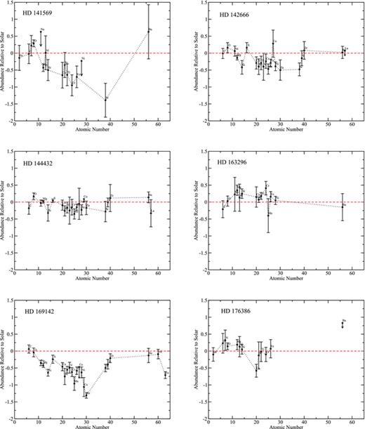
Final abundances relative to solar for the stars in this study, as in Fig. A1.
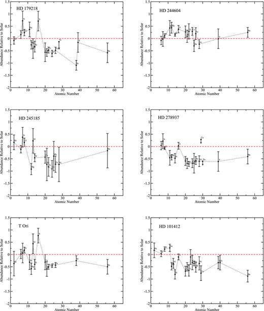
Final abundances relative to solar for the stars in this study, as in Fig. A1.
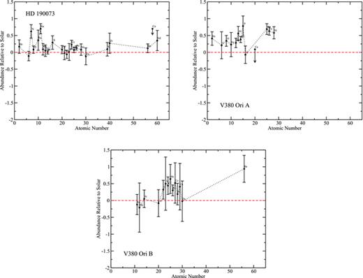
Final abundances relative to solar for the stars in this study, as in Fig. A1.
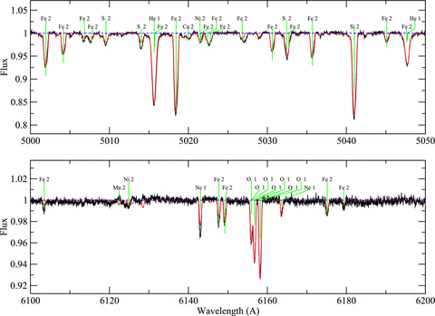
Comparison of the observed spectrum (jagged line) to the best-fitting synthetic spectrum (smooth line) for π Cet (HD 17081). Two independent wavelength regions are presented. Lines have been labelled by their major contributing species. Gaps in the synthetic spectra indicate regions that were not fit.
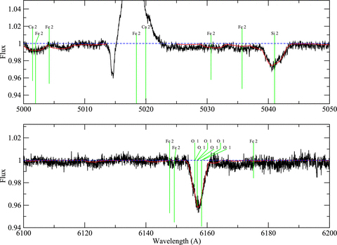
Comparison of the observed spectrum to the best-fitting synthetic spectrum for HD 31293, as in Fig. A5.
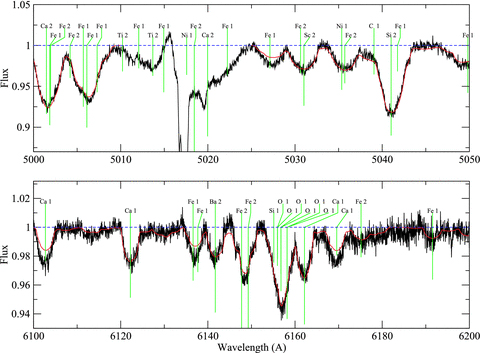
Comparison of the observed spectrum to the best-fitting synthetic spectrum for HD 31648, as in Fig. A5.
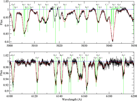
Comparison of the observed spectrum to the best-fitting synthetic spectrum for HD 36112, as in Fig. A5.
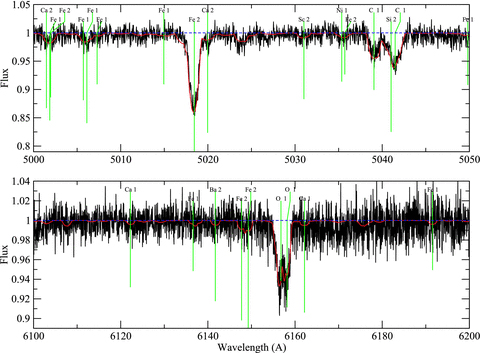
Comparison of the observed spectrum to the best-fitting synthetic spectrum for HD 68695, as in Fig. A5.

Comparison of the observed spectrum to the best-fitting synthetic spectrum for HD 139614, as in Fig. A5.
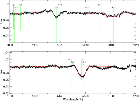
Comparison of the observed spectrum to the best-fitting synthetic spectrum for HD 141569, as in Fig. A5.
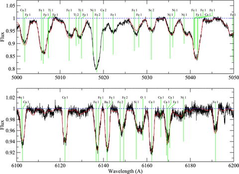
Comparison of the observed spectrum to the best-fitting synthetic spectrum for HD 142666, as in Fig. A5.

Comparison of the observed spectrum to the best-fitting synthetic spectrum for HD 144432, as in Fig. A5.
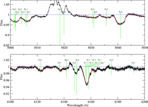
Comparison of the observed spectrum to the best-fitting synthetic spectrum for HD 163296, as in Fig. A5.
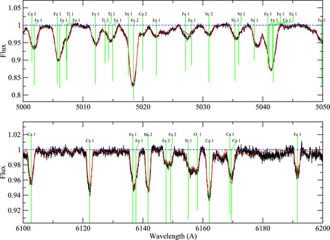
Comparison of the observed spectrum to the best-fitting synthetic spectrum for HD 169142, as in Fig. A5.
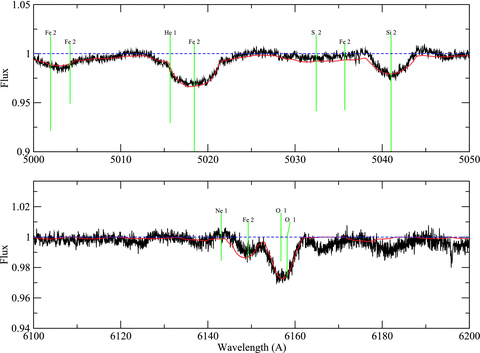
Comparison of the observed spectrum to the best-fitting synthetic spectrum for HD 176386, as in Fig. A5.
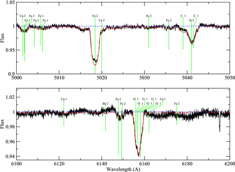
Comparison of the observed spectrum to the best-fitting synthetic spectrum for HD 179218, as in Fig. A5.
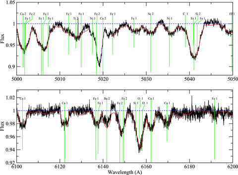
Comparison of the observed spectrum to the best-fitting synthetic spectrum for HD 244604, as in Fig. A5.
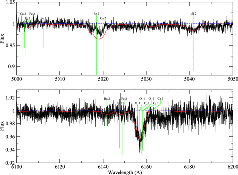
Comparison of the observed spectrum to the best-fitting synthetic spectrum for HD 245185, as in Fig. A5.
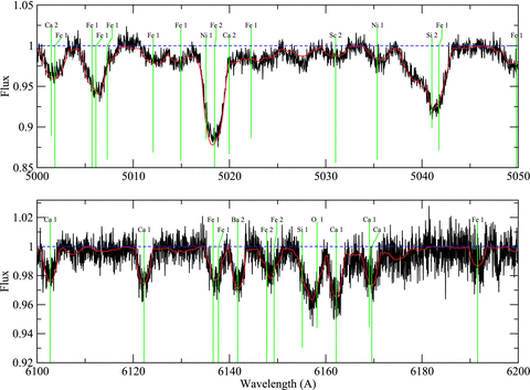
Comparison of the observed spectrum to the best-fitting synthetic spectrum for HD 278937, as in Fig. A5.
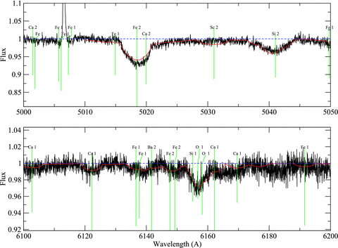
Comparison of the observed spectrum to the best-fitting synthetic spectrum for T Ori, as in Fig. A5.

Comparison of the observed spectrum to the best-fitting synthetic spectrum for HD 101412, as in Fig. A5.
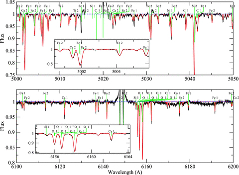
Comparison of the observed spectrum to the best-fitting synthetic spectrum for HD 190073, as in Fig. A5.
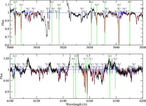
Comparison of the observed spectrum (jagged line) to the best-fitting synthetic spectrum of the combined V380 Ori A and B system (smooth line). The upper two rows of line labels (green) indicate lines of the primary, the lower two rows (blue) indicate lines of the secondary. Gaps in the synthetic spectrum indicate regions that were excluded from the fit.
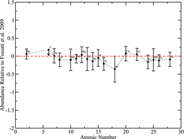
The difference between our final abundances and those of Fossati et al. (2009) for π Cet. A good agreement between the two sets of abundances is found.
5 TRENDS
We plotted the index [P] against effective temperature, mass, age and fractional pre-main-sequence age, as shown in Fig. 3. No clear trends were found, with a large scatter in chemical abundance at most temperatures, masses and ages. This peculiarity index was also compared to stellar radius, vsin i and microturbulence, but again no clear trends were found. Thus we conclude that the λ Boo peculiarities that we see are not restricted to a narrow mass range, and that they are present throughout the pre-main sequence.
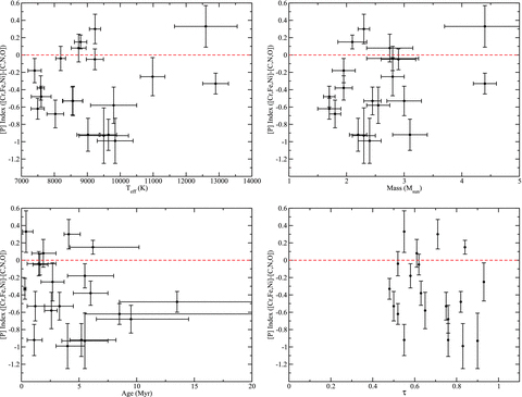
Trends in stellar parameters with the peculiarity index. The index is the average of Cr, Fe and Ni abundances each relative to solar, minus the average of the C, N and O abundances relative to solar. Plots are included for effective temperature, mass, age and fractional pre-main-sequence age (τ).
6 DISCUSSION
6.1 λ Boo peculiarities
The most striking result of this study is the discovery of a large number of HAeBe stars with moderate λ Boo-type chemical peculiarities. This trend seems to be present in both stars with and without detected magnetic fields, as shown by HD 101412. We find seven stars showing fairly strong λ Boo peculiarities, and another four stars with weaker λ Boo peculiarities, while eight stars are chemically normal and one is rather uncertain but appears to be normal. With the derived abundances, we see a continuous distribution of λ Boo peculiarities, from fairly strong to nearly undetectable. This incidence of roughly 50 per cent is much higher than the incidence of λ Boo stars on the main sequence of roughly 2 per cent (Paunzen 2001). While a detection rate of 50 per cent may be an overestimate (since our sample is biased towards stars with limited emission in their optical spectra), the true incidence of λ Boo peculiarities in HAeBe stars certainly is much higher than observed on the main sequence, suggesting an important connection with the pre-main-sequence evolutionary phase.
The sample of stars in our study is biased towards stars with weaker circumstellar emission or absorption in their spectra, since these stars allow for a more complete analysis of their photospheric spectra. However, the stars were drawn from the larger sample of Alecian et al. (2012a) which did not have this bias. We found 65 per cent of the stars in their sample had modest amounts of circumstellar contamination, and would have been suitable for our photospheric analysis. Thus, as a lower limit, 33 per cent of HAeBe stars should show λ Boo peculiarities, assuming that all the unsuitable stars in the sample of Alecian et al. (2012a) are chemically normal, and using our derived incidence of peculiarities for the suitable stars. The true incidence is likely higher than this lower limit.
There are almost certainly more undetected λ Boo stars in the sample of Alecian et al. (2012a) that we did not analyse, simply because analysing their complete sample was beyond the scope of this study. Indeed Alecian et al. (2012a) mention that HD 34282 appears to have weak lines of iron peak elements, but a normal O line. To roughly estimate the number of potential λ Boo stars in the remaining sample, we compared synthetic spectra computed using literature values for their atmospheric parameters and assuming solar abundances with the ESPaDOnS observations. In doing so we identified five additional stars that have suspiciously weak metal lines for their literature temperatures: HD 37806, HD 98922, HD 144668, HD 76534 and VX Cas. If all these stars do indeed show λ Boo peculiarities, 35 per cent of the stars observed with ESPaDOnS by Alecian et al. (2012a) would be λ Boo stars, which is consistent with our results.
This large incidence of λ Boo-type peculiarities in HAeBe stars is qualitatively consistent with a selective accretion model of λ Boo stars. HAeBe stars have recently undergone accretion, and may still be accreting, so it is reasonable that a process which depends on accretion is seen more frequently in these stars. Thus we consider our results supportive of the selective accretion model of λ Boo stars.
The large number of pre-main-sequence λ Boo stars we find suggests that the majority of λ Boo stars may develop their peculiarities on the pre-main sequence by accreting their circumstellar material. However, we cannot rule out the existence more of evolved λ Boo stars that only develop peculiarities on the main sequence, by accreting from diffuse interstellar clouds. Because of the relatively short lifetime of λ Boo peculiarities after accretion has halted, the presence of such peculiarities later in the main sequence (e.g. Paunzen et al. 2002) may require a different source of accreted material from that of pre-main-sequence λ Boo stars.
Turcotte & Charbonneau (1993) modelled the diffusion of chemical elements in the atmosphere of a star (with Teff= 8000 K and log g= 4.3) that was accreting gas depleted in iron peak elements. They found that λ Boo peculiarities can be generated quickly (∼0.1 Myr), but also dissipate quickly after accretion has stopped (∼1 Myr). This implies that, in the context of selective accretion, there is a good chance that HAeBe stars with λ Boo peculiarities are still accreting, or were very recently accreting.
The range in strengths of the λ Boo peculiarities seen in the stars in our sample might be interpreted as the consequence of different accretion rates in the stars. However, Turcotte & Charbonneau (1993) do not find a strong impact on surface abundances from different accretion rates, as long as they are sufficient to overwhelm diffusion and rotational mixing.
Alternately, the differences in the strengths of peculiarities could reflect the abundances of the accreted gas. These differences being due, for example, to the efficiency with which iron peak elements are bound into dust grains, or to the degree to which dust is blown away from the star while gas is accreted.
In this context, the chemically normal stars are most likely not accreting significant amounts of material, and thus any λ Boo peculiarities have dissipated. However, it is possible that accretion is ongoing but the selection process in the circumstellar material has broken down. For example, dust grain formation may not be proceeding efficiently, and thus the accreted gas would not be depleted in iron peak elements.
Unfortunately, deriving accretion rates for HAeBe stars is not a simple process. For example, Donehew & Brittain (2011) measured accretion rates based on Balmer jump excess fluxes. They obtained values between a few 10−7 and 10−8 M⊙ yr−1. These values rely on models from Muzerolle et al. (2004), which are constructed assuming magnetospheric accretion. Given the absence of detectable magnetic fields in most of the stars in our study, magnetospheric accretion may not be an accurate model (see Wade et al. 2007), and thus these accretion rates may not be accurate either. Generally, accretion rates derived for HAeBe stars are based on rather simple models, and thus it is not clear how reliable those accretion rates are. 11 of the stars in our sample have measured accretion rates by Donehew & Brittain (2011). Supplementing these results with accretion rates from Mendigutía et al. (2011), who used a similar methodology, and from Garcia Lopez et al. (2006), who based their accretion rates on Brγ emission, provides literature values for 15 stars in our sample. Worryingly, the literature accretion rates differ for five of these stars by between 0.5 and 1 dex. Whether this apparent disagreement is due to intrinsic stellar variability, differences in methodology or simply large uncertainties is not clear (Mendigutía et al. 2011). We compare these accretion rates with our peculiarity index [P] (defined in Section 5), stellar mass and fractional pre-main-sequence age in Fig. 4. In cases where multiple accretion rates are available the average value was taken. V380 Ori was left out of the comparison due to its binarity. We see no correlation between accretion rate and chemical peculiarity or mass. There is possibly a weak correlation with fractional pre-main-sequence age, but due to the large uncertainties on both the accretion rates and the fractional ages it is not entirely clear.

Trends in stellar parameters with literature accretion rates. Plots are included for our chemical peculiarity index, stellar mass and fractional pre-main-sequence age (τ).
Our results provide further evidence against the hypothesis that λ Boo stars are formed by radiative diffusion with mass loss, as proposed by Michaud & Charland (1986). In their calculations, Michaud & Charland (1986) find that it takes 108 or 109 yr to build up λ Boo peculiarities by diffusion in the presence of mass loss. This is much greater than the ages of the λ Boo-like stars in our sample, which are only a few × 106 yr old. Thus the time-scale for this mechanism is dramatically incompatible with our observations. This is consistent with the generally accepted view that diffusion with mass loss is insufficient for producing λ Boo peculiarities (e.g. Charbonneau 1993).
6.2 Magnetic stars
The one possible Bp star in our sample is V380 Ori A. This star shows modest overabundances of Fe, Mn and Ni of ∼0.6 dex, and Si is also enhanced relative to solar. C, Ne and S are consistent with solar, as are O and Mg at 2σ. This pattern is characteristic of Ap/Bp stars. Arguably, results are marginally consistent with the star simply having a high metallicity (∼0.4 dex above solar). However, since Fe, Mn and Ni are more enhanced than 0.4 dex, and C, O, Ne, Mg and S are less enhanced than this, we consider it more likely that the star is weakly chemically peculiar. If the star is a Bp star, the star has begun developing Ap/Bp chemical peculiarities, but they have not yet reached the degree seen in most main-sequence Ap and Bp stars.
Atomic diffusion producing chemical peculiarities was modelled in V380 Ori A by Vick et al. (2011), using a model that includes stellar evolution, as well as mass loss and atomic diffusion. They used the stellar parameters determined by Alecian et al. (2009), who find a somewhat lower mass than we do (mostly due to assuming RV= 3 rather than 5, thus using less extinction). Nevertheless, the abundances they derive should be roughly representative. Vick et al. (2011) find Mn, Fe and Ni to be overabundant by ∼0.5 dex, which agrees nicely with our results. They find roughly solar abundances for C, O and S, which agrees with our results. The overabundance of P that they find is also roughly consistent with our results. However, the underabundant Mg, and solar Si abundance that they find are inconsistent with our results. Thus, while this model is imperfect, we find it does provide a reasonable approximation of the majority of the observed peculiarities in V380 Ori A.
Interestingly, HD 190073 and HD 101412 are both magnetic but do not show Ap/Bp chemical peculiarities. HD 190073 is chemically normal, while HD 101412 shows λ Boo-type chemical peculiarities. Thus, unlike on the main sequence, not all pre-main-sequence magnetic A and B stars are chemically peculiar. Atomic diffusion theory suggests that enough time must elapse after accretion and deep surface convection have halted for significant peculiarities to develop. The dissipation of a large convective envelope can be modelled easily enough, and in most models dissipates early in pre-main-sequence life of A and B stars. However, determining when accretion has dropped sufficiently for atomic diffusion to dominate is much harder. Indeed it may depend on the circumstellar environment of the particular star, and thus not be reliably predictable.
The λ Boo peculiarities of HD 101412 presumably simply reflect the high incidence of λ Boo peculiarities in HAeBe stars in general. Thus, we suspect that these peculiarities are not a consequence of the magnetic field of HD 101412.
Modelling by Vick et al. (2011) suggests that HD 190073 has not yet had time to develop Ap/Bp chemical peculiarities. In their models, a star of this mass requires ∼2 Myr to develop peculiarities by atomic diffusion, while we find HD 190073 is only  Myr old. HD 101412 has almost the same mass, and we find an age of only
  Myr, thus by the models of Vick et al. (2011) it is also too young to have developed Ap/Bp peculiarities. The younger age of HD 101412 is consistent with the picture of its λ Boo-type chemical peculiarities being due to selective accretion, since accretion is more likely to be ongoing earlier in a stars life.
It is interesting that the two stars in this sample with the largest amount of emission in their optical spectra are V380 Ori A and HD 190073, both of which are magnetic. In particular, the emission mostly appears in lines that would be strongly in absorption for a purely photospheric spectrum of the star. HD 101412, the third magnetic star, displays a fairly modest amount of emission. Additionally, the measured accretion rates for V380 Ori and HD 190073 are both substantially higher than for other stars in our sample [ for V380 Ori,
  for HD 190073; Donehew & Brittain 2011; Mendigutía et al. 2011]. The impact of the secondary in V380 Ori does not appear to be considered in the measurement of the star’s accretion rate, and thus it may be somewhat inaccurate. In classical T Tauri stars, the strong emission in their spectra is thought to result from magnetically channelled accretion flows falling on to the star. We speculate that the strong emission in V380 Ori A and HD 190073 might be produced by a similar process. However, it is not clear whether this is the case, both because of the small sample size, and because the non-magnetic stars in the sample are biased towards lower emission stars (since large amounts of emission limit the abundance analysis). Magnetic fields are not detected in individual emission lines for any of our stars, thus we cannot use those lines to assess the presence of magnetospheric accretion directly.
The three stars in our sample with confirmed magnetic fields also have the lowest vsin i values (for more analysis see Alecian et al. 2012b). In this respect these three magnetic HAeBe star are similar to Ap/Bp stars, which rotate slower than normal non-magnetic A and B stars. The low vsin i of the magnetic HAeBe stars HD 200775A (vsin i= 26 ± 2 km s−1; Alecian et al. 2008a) and of NGC 2244 OI 201 (vsin i= 23.5 ± 0.5 km s−1; Alecian et al. 2008b), and the moderate vsin i of HD 72106 A (vsin i= 41.0 ± 0.6 km s−1; Folsom et al. 2008) support this observation. However, the very high vsin i of NGC 6611 W610 (vsin i= 190 ± 10 km s−1; Alecian et al. 2008b) indicates that not all magnetic HAeBe stars rotate slowly. Nevertheless, the large number of low vsin i magnetic HAeBe stars suggests that magnetic braking may have occurred in many of these stars (see Alecian et al. 2012b).
Several other very young magnetic A and B stars are known to have chemical peculiarities. Folsom et al. (2008) examined the magnetic star HD 72106 A, and found Ap/Bp peculiarities. They find that the star has a mass of 2.4 M⊙. While they were unable to firmly conclude that HD 72106 A is on the pre-main sequence, they do find that the system is between 6 and 13 Myr from the birthline, based on the H–R diagram position of the secondary in the binary system. The pattern of abundances seen in HD 72106 A is similar to that seen in V380 Ori A, but more extreme. Overabundances of iron peak elements and a weak overabundance of Si is seen in both stars. However, the strong He underabundance seen in HD 72106 A is not seen in V380 Ori A. The differences in abundances between the stars could be due to V380 Ori A being hotter and more massive HD 72106 A, or due to HD 72106 A being more evolved.
Bagnulo et al. (2004) investigated the main-sequence magnetic star NGC 2244−334, which is a member of the open cluster NGC 2244, and found Ap/Bp peculiarities. They found that the star has a mass of ∼4 M⊙ and commented that, as a cluster member, the star is likely ∼2 Myr old as measured from the ZAMS. This is a similar mass to V380 Ori A, though NGC 2244−334 is somewhat older. The peculiarities they found are very similar to those of HD 72106 A, with overabundances in iron peak elements of 1–2 dex, a somewhat weaker overabundance of Si, and a strongly underabundant He. This is again similar to what we see in V380 Ori A, though much stronger, and with a He underabundance.
Alecian et al. (2008b) studied the magnetic Herbig Be star NGC 6611 W601, and noted peculiarly strong He and Si lines in its spectrum. This suggests the star likely represents a pre-main-sequence He-strong star, but a detailed abundance analysis has yet to be performed. While this pattern of peculiarities would be different from that of V380 Ori A, the star has a much higher temperature of 22500 ± 2500 K and a much higher mass of  M⊙ (Alecian et al. 2008b). For a main-sequence magnetic star in this temperature and mass range, one would expect to see He-strong peculiarities, rather than Ap/Bp peculiarities. Alecian et al. (2008b) estimate the age of NGC 6611 W601 to be less than 0.06 Myr from the birthline of Palla & Stahler (1993, for an accretion rate of 10−4 M⊙ yr−1), based on its H–R diagram position. While this is very young, there are no models from Vick et al. (2011) for a comparable mass. We do note, however, that Vick et al. (2011) find peculiarities developing faster for more massive models.
Thus, while the peculiarities seen in V380 Ori A are weak, the pattern of peculiarities is consistent with those seen in other young intermediate-mass magnetic stars. This is consistent with the hypothesis that the weak peculiarities we see in this star will develop into the stronger peculiarities seen in most main-sequence Ap/Bp stars.
6.3 Chemically normal stars
We find no hints of any chemical peculiarities in the stars of our sample other than λ Boo peculiarities and the weak Bp peculiarities in V380 Ori A. Thus we find no evidence for Am or HgMn stars on the pre-main sequence. Our sample is not large enough to definitively exclude the existence of Am and HgMn stars at the same incidence as on the main sequence. However, if the roughly 10–20 per cent incidence (e.g. Smith 1996) of these stars on the main sequence is extended to the pre-main sequence, we would expect to have seen two to four such stars. Thus it is possible that these peculiarities do not form on the pre-main sequence, unlike for Ap/Bp stars. The atomic diffusion thought to give rise to these peculiarities may be disrupted by weak accretion more readily than the diffusion in the presence of a magnetic field that produces Ap/Bp stars. The presence of a magnetic field may stabilize a stellar atmosphere and increase diffusion velocities, potentially making diffusion in the presence of a magnetic field more robust (Michaud 1970; Michaud, Charland & Megessier 1981). Alternately, diffusion in non-magnetic stars may simply require more time than the pre-main-sequence lifetime of these stars to produce significant peculiarities.
The large majority of young A and B stars analysed, both on the main sequence and on the pre-main sequence (e.g. Acke & Waelkens 2004), have been found to be chemically normal. A very precise study of A and B star abundances by Fossati et al. (2009) investigated what ‘normal’ abundances are for A and B stars. They found that solar abundances are a good approximation, though there were small deviations for specific elements, which appeared to depend on the temperature of the star. Studies of nearby open clusters support this conclusion (e.g. Fossati et al. 2008, 2011; Villanova, Carraro & Saviane 2009).
Acke & Waelkens (2004) performed an abundance analysis of 24 pre-main-sequence and very young main-sequence stars, based on equivalent widths. A comparison of individual results for the seven stars we have in common with their study is discussed in Appendix A. Our results are generally consistent, although we are able to determine abundances for a wider range of elements, and in many cases provide more precise abundances. The one notable difference in our results is for HD 139614. For this star our more accurate Teff allows us to classify the star as λ Boo, while Acke & Waelkens (2004) could only comment that it appeared to be metal weak. In total Acke & Waelkens (2004) found only one Herbig star that was also a clear λ Boo star (HD 100546), and they noted that AB Aur shows hints of λ Boo peculiarity. In part this difference in detection rates may due to our more accurate Teff and log g values, as the case of HD 139614 demonstrates. Our higher precision, due to an improved methodology and higher S/N observations, is also a significant part of this difference. Finally, both our studies deal with a fairly small number of stars, and thus the true incidence of λ Boo peculiarities in HAeBe stars remains somewhat uncertain.
6.4 Possible veiling
One concern when analysing spectra of T Tauri stars is veiling. Veiling is additional continuum emission, usually from an accretion shock (or other circumstellar material), which makes spectral lines appear weaker than they would in a purely photospheric spectrum. In HAeBe stars, veiling can be seen in the ultraviolet (e.g. Donehew & Brittain 2011), but usually is considered to be unimportant in the optical (e.g. Böhm & Catala 1993; Hernández et al. 2004; Cowley et al. 2010; Donehew & Brittain 2011). HAeBe stars are intrinsically much more luminous than T Tauri stars, thus much more emission from an accretion shock would be needed to have the same veiling effect. Measured accretion rates for HAeBe stars are usually not much larger than for T Tauri stars, thus it is unlikely that HAeBe stars would have much larger amounts of emission from accretion shocks. Consequently, we would not expect veiling to have much impact on HAeBe star spectra.
If veiling is present in our observations it could make a star appear to be metal poor when it is not, thus it is important to check for veiling. If it is present in our spectra, veiling should have some wavelength dependence. We have compared abundances derived from different wavelength regions for individual stars. No clear correlation of abundance with wavelength was found, suggesting that veiling is unimportant in these stars. Veiling should affect all lines in a wavelength region similarly. Thus, if it is present veiling should affect most elements similarly, since the lines for most elements are widely distributed in our spectra. In particular, it could not produce underabundances in iron peak elements while keeping solar abundances of C and O that we see in many of the stars in our sample. Therefore veiling should not affect the relative abundances of C, N and O to Fe, even if it were present at a significant level in our spectra. We conclude it is unlikely that veiling has a significant impact on our derived abundances, and even if veiling is present it is not obvious how it could produce peculiar abundance patterns.
Arguably, the pattern of λ Boo underabundances we observe could be due to weak emission infilling in all the lines of some elements, however, this is very unlikely. We have searched carefully for emission in lines, both by looking for unexpected variability and by looking for lines with shapes inconsistent with rotational broadening. Thus we have excluded most if not all lines with emission. More importantly, lines of an element with lower excitation potentials are more likely to have stronger emission, thus emission would not be uniform across all lines. If emission infilling was occurring and otherwise undetected, we would observe it as an inability to simultaneously fit a wide range of lines of one element with one abundance. We do not find this, and consequently can safely conclude that the λ Boo peculiarities we detect are real, and not simply due to emission infilling.
7 CONCLUSIONS
We have performed a detailed abundance analysis of 21 stars, 20 of which are HAeBe stars, one of which (π Cet) is not a Herbig star, but may still be on the pre-main sequence. Three of these stars have confirmed magnetic fields, while magnetic fields do not appear to be present at detectable levels in the remaining 18.
We find nine stars that are chemically normal (one of which is rather uncertain), 11 that show λ Boo chemical peculiarities, and one that is weakly Ap/Bp. This is a remarkably large fraction of stars that display λ Boo-type peculiarities. On the main sequence, only ∼2 per cent of stars display λ Boo peculiarities (Paunzen 2001). We interpret this as evidence in favour of a selective accretion hypothesis for the development of λ Boo peculiarities. Since Herbig stars are either accreting or have recently finished accreting, a process which depends on accretion should be seen more frequently in these stars.
Of the three magnetic stars, HD 101412 displays λ Boo peculiarities, HD 190073 is chemically normal and V380 Ori is weakly Bp. Thus it appears that magnetic Herbig stars can display Ap/Bp-type peculiarities, but not all magnetic Herbig stars do. This is in contrast to main-sequence magnetic A and late B stars, which always display Ap/Bp-type peculiarities (Aurière et al. 2007). The presence of λ Boo peculiarities in a magnetic star appears to simply reflect the high incidence of these peculiarities in all Herbig stars.
GAW and JDL are supported by Natural Science and Engineering Research Council (NSERC Canada) Discovery Grants, and GAW is also supported by a Department of National Defence (Canada) ARP grant.
REFERENCES
Appendix
APPENDIX A: RESULTS FOR INDIVIDUAL STARS
A1 Non-magnetic stars
A1.1 π Cet (HD 17081)
The best-fitting abundances for the stars in this study are plotted, relative to solar abundances, in Figs A1, A2, A3 and A4. Examples of these fits are provided for each star in Figs A5 through A24. π Cet (HD 17081) is a cool B star that was studied in detail by Fossati et al. (2009). They performed a very precise, detailed abundance analysis, and considered the star to be a good example of a ‘normal’ cool B star. π Cet is not a Herbig Be star by the strict definition, since it has no strong emission in its optical spectrum. However, the star does display an infrared excess (Malfait, Bogaert & Waelkens 1998), as well as some unexplained line profile variations (Fossati et al. 2009), and an H–R diagram position to the right of the main sequence. Thus the star is certainly very young, and possibly still on the pre-main sequence, despite the lack of clear emission. Based on the H–R diagram position of the star, it appears to be less than 0.5 Myr from the birthline, and almost certainly is less than 1 Myr old. Malfait et al. (1998) suggested this star was a Vega-type star, a classification which is consistent with our observations.
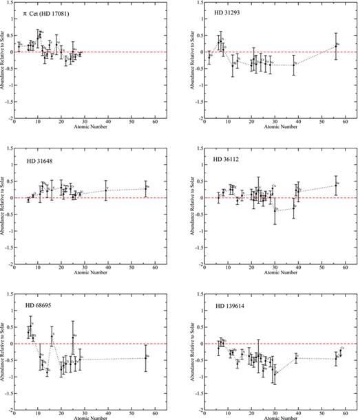
Final abundances relative to solar for the stars in this study. Solar abundances are taken from Grevesse et al. (2005). Points marked with an arrow represent upper limits only.
In order to check the accuracy of our methodology, we analysed an observation of π Cet and compared our results with the results of Fossati et al. (2009). Our results are completely consistent with those of Fossati et al. (2009), for temperature, gravity, vsin i and abundances. Our atmospheric parameters and abundances are compared with those of Fossati et al. (2009) in Table A1, and the differences between our abundances and those of Fossati et al. (2009) are plotted in Fig. A25. The excellent agreement between our results and Fossati et al. (2009) demonstrates the accuracy of our methodology.
Our results compared with those of Fossati et al. (2009) for π Cet.
| Fossati et al. (2009) | This work | |
| Teff (K) | 12 800 ± 200 | 12 900 ± 400 |
| log g | 3.75 ± 0.1 | 3.8 ± 0.2 |
| vsin i (km s−1) | 20.2 ± 0.9 | 20.9 ± 1.2 |
| ξ (km s−1) | 1.0 ± 0.5 | 1.7 ± 1.0 |
| He | −0.97 ± 0.04 | −0.91 ± 0.14 |
| C | −3.58 ± 0.07 | ≤− 3.4 |
| N | −4.03 ± 0.13 | −4.03 ± 0.15 |
| O | −3.06 ± 0.14 | −3.16 ± 0.13 |
| Ne | −3.66 ± 0.09 | −3.76 ± 0.28 |
| Na | −5.23 ± 0.07 | −5.3 ± 0.1 |
| Mg | −4.47 ± 0.16 | −4.43 ± 0.15 |
| Al | −5.73 ± 0.27 | −5.81 ± 0.17 |
| Si | −4.41 ± 0.2 | −4.55 ± 0.14 |
| P | −6.38 ± 0.19 | −6.43 ± 0.14 |
| S | −4.78 ± 0.16 | −4.99 ± 0.08 |
| Ar | −5.24 ± 0.19 | −5.6 ± 0.3 |
| Ca | −5.77 | −5.7 ± 0.2 |
| Ti | −7.42 ± 0.08 | −7.37 ± 0.15 |
| Cr | −6.41 ± 0.1 | −6.57 ± 0.16 |
| Mn | −6.5 ± 0.09 | −6.6 ± 0.3 |
| Fe | −4.58 ± 0.14 | −4.70 ± 0.08 |
| Ni | −5.76 ± 0.19 | −5.85 ± 0.06 |
π Cet was observed spectropolarimetricly by Wade et al. (2007), who did not detect a magnetic field. Alecian et al. (2012a) also found no magnetic field in π Cet, and thus we consider the star to be non-magnetic.
A1.2 HD 31293 (AB Aur)
We derive Teff= 9800 ± 700 K and log g= 3.9 ± 0.3 for HD 31293 (AB Aur). This Teff is consistent with Acke & Waelkens (2004), but our log g is inconsistent with their (remarkably high) value of 5.0. The Teff and log g are both consistent with Böhm & Catala (1993). We find solar He and O abundances, C and N are 1σ above solar, while the iron peak elements are consistently 1σ below solar. The systematic underabundance of iron peak elements by ∼0.3 dex suggests the star may be a weak λ Boo star. This is strengthened somewhat by the observation that the iron peak elements are ∼0.5 dex below the average C, N and O abundance. Based on these underabundances, we conclude that the star most likely is a weak λ Boo star, but it is a marginal case.
Acke & Waelkens (2004) derive abundances for O, N and Si that are consistent with ours, but their Fe abundance of 1 dex below solar (based on two Fe i lines) is inconsistent with our value. This difference may be due to the higher log gAcke & Waelkens (2004) used. Alternately, it is possible their measurement was impacted by the large amount of emission in the spectrum of HD 31293. Both Fe abundances are consistent with a λ Boo classification of the star, but we prefer our larger abundance since it is based on larger number and a wider range of lines, and it is consistent with the neighbouring iron peak element abundances we derive.
Alecian et al. (2012a) find no magnetic field in HD 31293. Wade et al. (2007) also find no magnetic field in this star, thus we consider it to be non-magnetic.
A1.3 HD 31648
For HD 31648 we derive an Teff of 8800 ± 190 K and a log g of 4.1 ± 0.2, which is consistent with Acke & Waelkens (2004). We find most abundances within 1σ of solar, and all abundances except Mg and Ti within 2σ. The abundances are systematically slightly above solar and may reflect a slightly enhanced metallicity, or a slightly overestimated Teff.
Our Ca and Fe abundances are consistent with Acke & Waelkens (2004), our C abundance is consistent at 2σ, as is our Y abundance if we assume the uncertainty on their value is comparable to ours. Our Si and Mg abundances are not consistent with Acke & Waelkens (2004), although their abundances are based on only one line and thus are likely uncertain. The large vsin i of this star causes significant blending in its spectrum. This could explain the discrepancies between our results, since the Acke & Waelkens (2004) abundances are based on equivalent width measurements, which can easily be influenced by unaccounted-for blending.
HD 31648 was not found to have a magnetic field by Alecian et al. (2012a). No magnetic field was found by Wade et al. (2007) either. Hubrig et al. (2006) claimed a weak detection of a magnetic field in their observation of HD 31648 but, in the re-reduction of the observation made by Hubrig et al. (2007) the field is below their detection threshold. Surprisingly, Hubrig et al. (2007) report a signal the Hβ, Hγ, Hδ and Ca H&K lines of their V/I spectrum, which they interpret as a ‘circumstellar’ magnetic field. This result has yet to be independently confirmed. A careful examination of the Hβ, Hγ, Hδ and Ca H&K lines in our spectra shows no polarization signature. Bagnulo et al. (2012) re-reduced a wide range of spectropolarimetric observations from the FORS1 instrument at the VLT, including the observations of Hubrig et al. (2006). They find no evidence for a magnetic field in HD 31648. Considering the lack of evidence for a photospheric magnetic field, and the absence of a confirmation of a ‘circumstellar’ magnetic field, we conclude that HD 31648 is non-magnetic.
A1.4 HD 36112
For HD 36112 we find Teff= 8190 ± 150 K and log g= 4.1 ± 0.4, both of which are somewhat greater than the Teff= 7750 and log g= 3.5 of Acke & Waelkens (2004). Our uncertainty on Teff may be overly optimistic, though it does reflect the scatter in Teff derived from different spectral windows. The uncertainties on the calibration of Teff become important at this level, and thus there may be some systematic uncertainty not included in our error bar. Most of our derived abundances are within 1σ of solar, and all are within 2σ. There are no systematic enhancements or depletions, thus we conclude HD 36112 is chemically normal, with solar abundances.
Our abundances are consistent with those of Acke & Waelkens (2004) for C, Si, S, Ca, Sc, Cr, Mn, Fe and Ni. Our abundance for Ti and Y differ by ∼2σ. These differences may be a consequence of our hotter temperature, or they may be due to the small number of lines Acke & Waelkens (2004) used for determining those abundances.
Alecian et al. (2012a) do not detect a magnetic field in this star. In their FORS1 observations Wade et al. (2007) do not detect a magnetic field, nor do Bagnulo et al. (2012) in their re-reduction of the FORS1 observations.
A1.5 HD 68695
For HD 68695 we derive Teff= 9000 ± 300 K and log g= 4.3 ± 0.3. We find C, N, O and S abundances that are ∼1σ above solar, while iron peak abundances are 2–3σ below solar (∼0.7 dex below solar), except for the rather uncertain Mn abundance. We conclude that this star has clear λ Boo peculiarities.
No magnetic field was detected in HD 68695 by either Alecian et al. (2012a) or by Wade et al. (2007), thus we consider the star to be non-magnetic.
A1.6 HD 139614
HD 139614 was analysed by Acke & Waelkens (2004) using an Teff of 8000 K. They found an overall deficiency of metals, but no clear evidence of the selective depletion characteristic of λ Boo stars. We find HD 139614 to have an Teff of 7600 ± 300 K, and a log g of 3.9 ± 0.3, which is consistent with the results of Teff= 7400 ± 200 K and log g= 4.0 ± 0.4 reported by Guimarães et al. (2006), and marginally consistent with Acke & Waelkens (2004) (at 1.3σ in Teff and 2σ in log g). We consider our parameters (and Guimarães et al. 2006) to be more accurate, since Acke & Waelkens (2004) values were based on the spectral classification of Malfait et al. (1998), which could be influenced by chemical peculiarities in the star. In fact, for our parameters we find a clear λ Boo pattern of abundances, with solar C, N and O, and underabundant iron peak elements.
No magnetic field was detected in HD 139614 by Alecian et al. (2012a). Hubrig, Schöller & Yudin (2004) claimed a detection of a magnetic field in this star, which was not supported by Wade et al. (2005). Further observations by Hubrig et al. (2009) did not detect a magnetic field in the star, though they comment on a possible signal in the Ca H&K lines. In their re-reduction of FORS data, Bagnulo et al. (2012) find no evidence for a magnetic field in HD 139614, and conclude that the reported detection by Hubrig et al. (2004) is likely spurious. Consequently, we consider HD 139614 not to have a significant magnetic field.
A1.7 HD 141569
We find Teff= 9800 ± 500 K and log g= 4.2 ± 0.4 for HD 141569, which is consistent with the parameters found by Guimarães et al. (2006). We find λ Boo peculiarities in this star, with solar He, C and N, possibly overabundant O, and underabundant iron peak elements.
Alecian et al. (2012a) do not detect a magnetic field in the star. Wade et al. (2007) also find no magnetic field, thus we conclude HD 141569 does not have a significant magnetic field.
A1.8 HD 142666
For HD 142666 we find Teff= 7500 ± 200 K and log g= 3.9 ± 0.3, which is consistent with Guimarães et al. (2006). We find weak λ Boo peculiarities in this star. C, O, Na and S have solar abundance, while the iron peak elements are consistently ∼0.5 dex below solar, except for the rather uncertain Co abundance.
Wade et al. (2007) observed the star and found no magnetic field. Alecian et al. (2012a) find no magnetic field in the star either.
A1.9 HD 144432
For HD 144432 we find Teff= 7400 ± 200 K and log g= 3.9 ± 0.3, which is consistent with Guimarães et al. (2006). The abundances of all elements we derive are within 2σ of solar, and most are within 1σ. There are no clear trends in abundances of different elements, thus we consider the star chemically normal, with nearly solar metallicity.
Alecian et al. (2012a) observed HD 144432 twice and found no magnetic field. Wade et al. (2007) also found no magnetic field in the star. Hubrig et al. (2007) claim a weak magnetic field detection in this star in one observation, but Hubrig et al. (2004, 2009) did not detect a significant magnetic field in the star. Bagnulo et al. (2012) re-reduced the one observation of HD 144432 with a magnetic field detection from Hubrig et al. (2007). Bagnulo et al. (2012) do find a magnetic field in the observation at a 4.9σ level (〈Bz〉=−108 ± 22 G). However, they caution that the impact of instrumental effects on the detection of weak magnetic fields is not well understood for the FORS1 instrument. They conclude that for weak magnetic fields, detections at less than 6σ should not be considered definite, and require supporting observations. Thus, while we cannot completely exclude the possibility of a magnetic field in HD 144432, based on the large majority of the evidence (five out of six observations) we conclude that HD 144432 likely has no significant magnetic field.
A1.10 HD 163296
We determine an Teff of 9200 ± 300 K and a log g of 4.2 ± 0.3, which is consistent with Guimarães et al. (2006). We find the abundances of most elements to be within uncertainty of solar, though Mg and Cr are both overabundant at slightly more than 2σ. With largely solar abundance and no clear selective depletion or enhancement, we conclude that the star is chemically normal.
Alecian et al. (2012a) do not find a magnetic field in HD 163296. Hubrig et al. (2009) also do not detect a magnetic field in the star, thus we conclude the star is non-magnetic.
A1.11 HD 169142
For HD 169142 we find Teff= 7500 ± 200 K, which is consistent with Guimarães et al. (2006), and log g= 4.3 ± 0.2, which is 2σ greater than Guimarães et al. (2006) who find log g= 3.7 ± 0.1. If we were to adopt the log g of Guimarães et al. (2006), it would decrease our abundances by between ∼0.05 and ∼0.2 dex depending on the element, which is generally within our uncertainties. We find a clear λ Boo pattern of abundances in this star. C and O are solar, and S is only slightly underabundant, while iron peak elements are underabundant by between 0.5 and 1 dex. Interestingly Ba and Nd are roughly solar, though Eu may be underabundant.
Alecian et al. (2012a) do not detect a magnetic field in HD 169142, nor do Hubrig et al. (2009).
A1.12 HD 176386
We derive an Teff of 11000 ± 400 K and a log g of 4.1 ± 0.3 for HD 176386. The abundances we derive for the star are consistent with solar, with the possible exception of Ca. Thus we conclude that the star is chemically normal.
No magnetic field was found for HD 176386 by Alecian et al. (2012a). Hubrig et al. (2009) claim a marginal detection at 3σ in one observation. Bagnulo et al. (2012) re-reduced this observation and found no magnetic field. Thus, based on the majority of the evidence, we consider HD 176386 to be a non-magnetic star.
A1.13 HD 179218
For HD 179218 we derived Teff= 9640 ± 250 K and log g= 3.9 ± 0.2, both of which are consistent with Guimarães et al. (2006). We find a solar He abundance, abundances of C, O and Na that are marginally enhanced relative to solar, and N and S abundances that are uncertain, but apparently enhanced relative to solar. Iron peak elements are depleted relative to solar by ∼0.5 dex. We conclude that HD 179218 displays λ Boo peculiarities. The overabundances of C, N, O and S may reflect an above solar intrinsic metallicity in the star, which the λ Boo peculiarities are superimposed upon. However, this is not certain, as He appears to have a nearly solar abundance.
Alecian et al. (2012a) find no magnetic field in HD 179218, which is supported by the non-detection of Hubrig et al. (2009).
A1.14 HD 244604
We found Teff= 8700 ± 220 K and log g= 4.0 ± 0.2 for HD 244604, which is consistent with the parameters from Acke & Waelkens (2004). We find most elements have solar abundances or are enhanced by around 1σ. There is no evidence for selective depletion or enhancement. We conclude that the star is chemically normal. Acke & Waelkens (2004) were only able to determine an iron abundance for HD 244604, though it is consistent with our abundance if we assume their uncertainty is similar to ours.
No magnetic field in HD 244604 is found by Alecian et al. (2012a). Wade et al. (2007) also find no magnetic field in the star, thus we consider the star to be non-magnetic.
A1.15 HD 245185
For HD 245185 we derive Teff= 9500 ± 750 K and log g= 4.0 ± 0.4, which is consistent with Acke & Waelkens (2004). We find He, C, N and O abundances that are consistent with solar, and iron peak abundances that are ∼0.8 dex below solar. While the uncertainties are relatively large for this star, the strong iron peak underabundances indicate λ Boo peculiarities. Acke & Waelkens (2004) were unable to determine any abundances for this star due to a low S/N in their observation and the high vsin i of the star.
Alecian et al. (2012a) do not detect a magnetic field in the star, nor do Wade et al. (2007). Consequently, we consider the star to be non-magnetic.
A1.16 HD 278937 (IP Per)
For HD 278937 (IP Per) we find Teff= 8000 ± 250 K and log g= 4.1 ± 0.2, which is consistent with the Teff of Miroshnichenko et al. (2001), though they derive a log g of 4.4 ± 0.1 which is 1σ above our value. The star is a known δ Scuti pulsator (Ripepi et al. 2006). We find solar abundances for C, N, O and S, while iron peak elements as well as Na, Mg and Si are between 0.5 and 0.7 dex underabundant. This star shows clear λ Boo peculiarities. Miroshnichenko et al. (2001) found that HD 278937 had a metallicity below solar ([M/H] =−0.4), based on a fit to the star’s metallic line spectrum. This value is most likely a result of the low iron peak abundances in the star, and thus consistent with our abundances. The solar abundances of C, N, O and S were likely overlooked by the scaled solar abundance model of Miroshnichenko et al. (2001) due to the relative scarcity of lines of those elements. Therefore, the star is not a low-metallicity star, but rather appears to have peculiar photospheric abundances.
No magnetic field is found in HD 278937 by Alecian et al. (2012a), or by Wade et al. (2007).
A1.17 T Ori
We find Teff= 8500 ± 300 K and log g= 4.2 ± 0.3 for T Ori. The abundances for He, C, N and O are all consistent with solar, while the S abundance is almost 3σ above solar. The S abundance is based only on two weak lines at 6749 and 6757 Å, and thus may be somewhat more uncertain than the error bar suggests. The iron peak abundances are clearly ∼0.5 dex below solar. We conclude that T Ori has clear λ Boo peculiarities.
Neither Alecian et al. (2012a) nor Wade et al. (2007) detect a magnetic field in T Ori.
A2 Magnetic stars
A2.1 HD 101412
HD 101412 was observed by Wade et al. (2005) and reanalysed by Wade et al. (2007) who found a longitudinal magnetic field of 500 ± 100 G. The presence of a magnetic field was recently confirmed by Hubrig et al. (2009, 2011) and Alecian et al. (in preparation). Cowley et al. (2010) derived chemical abundances for HD 101412, and surprisingly discovered it had λ Boo peculiarities. In our abundance analysis we find underabundances of iron peak elements, and solar C, O and He, with values that are consistent with those of Cowley et al. (2010). Thus we confirm that HD 101412 has λ Boo peculiarities. While in main-sequence A and B stars magnetic fields are associated with Ap and Bp chemical peculiarities, that is not the case for HD 101412.
We confirm the presence of an ‘anomalous saturation’ in the lines of HD 101412 noted by Cowley et al. (2010). Even with a microturbulence of 0 km s−1, when we fit weaker lines, stronger lines in the synthetic spectrum are often too deep to fit the observation. This problem is not consistent across all lines, and often appears to be fairly minor. This anomalous saturation does not appear to be common among HAeBe stars, as this is the only object for which we have seen this problem. A possible explanation for the discrepancy between the observations and the synthetic spectra is the presence of chemical stratification in the stellar atmosphere. Since stronger lines are often formed higher in the stellar atmosphere, if the abundance of some elements was lower, higher in the atmosphere that would explain the apparent weakness of many stronger lines. The possibility of stratification will be investigated in detail in a future paper. The presence of veiling in the spectrum of this star would produce a similar discrepancy to what we see, however, veiling would affect all lines of the same strength similarly, unlike the non-uniform trend we see. Thus we conclude veiling is unlikely to be the source of this discrepancy, in agreement with Cowley et al. (2010). The discrepancy is not likely to be a direct effect of the star’s magnetic field on line formation, which usually desaturates lines, and we do not find the problem in the other magnetic stars of our sample.
Placing HD 101412 on the H–R diagram, we find it has an age of  Myr and a mass of 3.0 ± 0.3 M⊙, both of which are consistent with Wade et al. (2007). Since the star has no Hipparcos parallax, we adopted the distance of 500–700 pc proposed by Vieira et al. (2003), however, this is somewhat uncertain. Even with this uncertainty, the star falls well before the beginning of the main sequence on the H–R diagram, thus the star is almost certainly a pre-main-sequence object.
We find similar λ Boo-type peculiarities in many of the non-magnetic HAeBe stars in our sample, thus this feature is not unique to HD 101412, or to magnetic HAeBe stars. Indeed, it appears that the peculiarities in HD 101412 occur in a significant fraction of all HAeBe stars.
A2.2 HD 190073
HD 190073 has a magnetic field, discovered and repeatedly detected by Catala et al. (2007), with a longitudinal strength of 74 ± 10 G that was constant over the course of their observations. In our analysis we find that the star is chemically normal, as shown in Fig. A4. Apparent over abundances relative to solar in N and Na may be due to non-LTE effects, or weak undiagnosed blends, since for both elements only a couple of very weak lines were usable for our analysis.
Acke & Waelkens (2004) analysed HD 190073 and adopted Teff= 9250 K and log g= 3.5, which is consistent with our values of Teff= 9230 ± 260 K and log g= 3.7 ± 0.3. Based on equivalent widths, they found abundances for C, N, O, Mg, Si, Ca, Sc, Ti, V, Cr, Fe, Ni Y, Zr and Ba, all of which are consistent with ours. For Al they found an abundance −0.45 dex below solar, based on only one line, which is inconsistent with our value. Our abundance is based on two lines, thus we consider it to be the more accurate value. Our result leads to a nearly solar abundance, consistent with other elements in this star.
We find that the star is quite young (1.6 ± 0.6 Myr), which agrees with the age determined by Catala et al. (2007) of 1.2 ± 0.6 Myr. Thus it is possible that the star has not yet had time to build up significant chemical peculiarities on its surface. This hypothesis is supported by the modelling of Vick et al. (2011), who found that it takes at least ∼2 Myr for a 2.9 M⊙ star to develop significant chemical peculiarities by radiative diffusion.
A2.3 V380 Ori A and B
V380 Ori is a triple star system, with two components detectable spectroscopically (Alecian et al. 2009). The more massive spectroscopic component (the primary) shows no detectable change in radial velocity, while the fainter, less massive (secondary) component’s radial velocity varies with a period of ∼100 d (Alecian et al. 2009). The third component in the system was detected by speckle interferometry in the infrared (Leinert, Richichi & Haas 1997), but is not detectable in the visible spectrum of the system (Alecian et al. 2009). The primary has a magnetic field, detected by Wade et al. (2005), while the secondary has no detectable magnetic field. The magnetic field of the primary was repeatedly observed by Alecian et al. (2009), who modelled the geometry as a dipole, with a strength of 2120 ± 150 G, and an obliquity of 66°± 5°.
Modelling the spectrum of the V380 Ori system was done somewhat differently than for the other stars in this study. Spectral disentangling was inapplicable due to the large amounts of variable emission in the spectrum, and the lack of radial velocity variation in the primary. Instead we fit a composite synthetic spectrum directly to the observation. The composite spectrum was constructed by adding the synthetic spectra of both stars, in absolute flux, weighted by the squared ratio of radii of the stars (the  dependence is included in the absolute fluxes of the synthetic spectra). The combined spectrum was then normalized by the sum of the continuum fluxes, also weighted by the ratio of radii squared. Using this composite spectrum, the model parameters for one star were simultaneously fit by χ2 minimization, while the other star’s parameters were held fixed. The ratio of radii was simultaneously fit as well, but the radial velocities of the two components were determined before the rest of the fitting process. The combination of parameters for both stars from one spectral window was determined iteratively, alternating between the two stars, and fitting the parameters of one while holding the parameters of the other fixed. Initial parameters were taken from Alecian et al. (2009).
We find chemical peculiarities in the primary that are consistent with Ap/Bp peculiarities. The peculiarities are weak, but detectable. C, S and Ne are within uncertainty of solar, while Fe, Ni and Mn are overabundant by more than 3σ. Si is also overabundant by more than 4σ in the primary, and He may be overabundant at 2.2σ. The abundances of the secondary are uncertain, but consistent with solar. Most elements in the secondary are within 1σ of solar, and all elements are within 2σ (except for Ba). The large uncertainty in the secondary stems mostly from the uncertainty in the ratio of radii (and hence ratio of luminosities) for the system, though uncertainties in effective temperature also play a role. While the average abundance in the secondary appears to be slightly above solar, it is not clear whether this reflects an intrinsically higher metallicity in the system, or if the luminosity ratio has simply been slightly overestimated. The abundances derived for the secondary are highly sensitive to the adopted ratio of radii, however, the abundances for the primary are not, since the primary dominates the luminosity of the system.
We find a ratio of radii for the V380 Ori system of RA/RB= 0.7 ± 0.1. The relatively large radius of the secondary is a consequence of the star being less massive, and thus being slower to contract towards the main sequence than the more massive primary. The H–R diagram positions of the two stars are consistent with a single isochrone.
The appearance of chemical peculiarities in the primary of V380 Ori is consistent with the modelling by Vick et al. (2011), who discuss this system in some detail. Since the primary is more evolved than HD 190073, it could have developed chemical peculiarities while HD 190073 has not yet.
