A new method for estimating frequency-dependent core shifts in active galactic nucleus jets Free

Abstract

1 INTRODUCTION

Most active galactic nuclei (AGN) display a ‘core+jet’ structure in Very Long Baseline Interferometry (VLBI) images. In the standard interpretation, the core is taken to be the optically thick base of the jet (Blandford & Königl 1979). Due to synchrotron self-absorption, the absolute position of the observed VLBI core (τ = 1 surface) shifts systematically with frequency, moving increasingly outward along the VLBI jet with lower frequency (Königl 1981). This frequency-dependent core shift has a direct effect on astrometric measurements performed in the radio and optical. In the near future, the GAIA astrometry mission and the Space Interferometry Mission will begin. For both missions, matching the optical astrometric catalogues to the radio catalogues (e.g. Fey et al. 2001) presents a very important problem. The core shifts can introduce offsets between the optical and radio positions of AGN of up to several milliarcsecond (Kovalev et al. 2008), which will strongly affect the accuracy of matching the radio and optical catalogues.

Core shifts are also needed for the correct reconstruction of VLBI spectral-index and rotation-measure maps. Moreover, knowledge of the frequency-dependent core shifts can be used to derive physical parameters of the jet, such as the core magnetic field and the distance from the VLBI core to the base of the jet (Lobanov 1998; Hirotani 2005).

Therefore, precise measurements of the core shifts are necessary. One way to obtain core shifts is through phase-referencing VLBI observations, however this is a complex and resource-intensive technique, and phase-referencing core shifts have been determined for only a few AGN, such as 1038+528 (Marcaide & Shapiro 1984), 4C 39.25 (Guirado et al. 1995), 3C 395 (Lara et al. 1994), 3C 390.1 (Ros & Lobanov 2001) and M 81 (Bietenholz, Bartel & Rupen 2004). Another indirect method to measure core shifts is to align optically thin parts of an AGN jet at different frequencies (e.g. Croke & Gabuzda 2008; Kovalev et al. 2008; O’Sullivan & Gabuzda 2009). However, this method requires simultaneous multifrequency VLBI observations, which are likewise fairly resource intensive, and does not always yield unambiguous results. The limitations of these techniques are exacerbated by the fact that the core shift may well depend on the activity state of an AGN, and therefore be time-dependent, whereas at present only isolated core-shift measurements for individual AGN are available. In addition, the magnitude of the core shifts that can be detected is limited by the resolution of the VLBI observations used.

In this paper, we discuss the opacity in the core regions of AGN and describe a new method for deriving core shifts from the frequency-dependent time lags of flares observed with single-dish observations. We use these time lags to derive physical parameters of the jets, such as the distance from the VLBI core to the base of the jet and the magnetic fields in the core region.

2 FREQUENCY-DEPENDENT TIME LAGS

The core is a compact feature in the VLBI map of an AGN with high brightness and a relatively flat spectrum, which is usually interpreted as that part of the jet where the optical depth τ is approximately unity. Since the τ = 1 surface has different locations at different frequencies (Königl 1981), the absolute position of the core should depend on the observing frequency. According to the standard shock-in-jet model, a change of electron density and pressure at the injection point near the base of the jet will cause a shock wave to propagate along the jet. This will cause brightening of the core region, which will be seen as a flare in the total flux density light curves, and will be followed by the appearance of a jet component (or components) in VLBI maps (e.g. Marscher & Gear 1985; Gómez et al. 1997). Consider a conical jet geometry (see Fig. 1) observed at a viewing angle φ. A shock wave appears at the distance R_on and then propagates along the jet. It will cross the τ = 1 surface for a particular frequency ν_i at some time T_i and emerge out of the core region. Since the position of the τ = 1 surface is shifted further from the jet base at lower frequencies, the times T_i will be delayed at lower frequencies. Fig. 1 shows how the T_i correspond to the maxima of the total flux density flares obtained with single-dish observations. Crossing the τ = 1 surface corresponds to a maximum of the total flux density outburst at the corresponding frequency, and the time of the flare maximum thus also depends on the frequency; thus, the time lags contain information about core opacity. According to the geometry of Fig. 1 and the principles of superluminal motion (e.g. Rees 1967; Türler, Courvoisier & Paltani 2000), the time t that has passed after the shock wave’s appearance at the distance R_on in the observer’s frame is

1

where R is the distance along the jet axis in the rest frame of the quasar, β_app is the apparent velocity in the plane of the sky in units of c, φ is the viewing angle, and z is the redshift of the source. In this equation, we assume that the apparent speed corresponds to the speed of the shock. Observing at multiple frequencies ν_a and ν_b, we can estimate the time lags between the maxima of the total flux density outburst:

2

3

Assuming that the shock wave appears at the same distance R_on at all frequencies, we obtain Δt(ν)_obs=ΔR_proj/β_appc, where ΔR_proj is the distance between R at the two frequencies projected on to the plane of the sky. Taking expression (33) for the frequency-dependent core shift from Hirotani (2005), we can write the dependence of the time lags on the frequency, spectral index α, magnetic field and electron density:

4

where

5

6

x_B is a dimensionless variable for B and f is a function of N₁, the spectral index and the viewing angle.

Figure 1

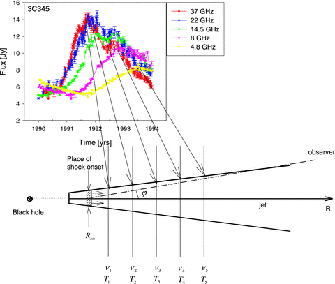
Sketch of the jet geometry discussed in Section 2 as observed in the rest frame of the quasar. The shaded rectangle shows a shock wave that starts at the distance R_on and propagates along the jet axis with the speed β. The vertical lines mark the core positions at different frequencies and the times when the shock wave reaches the core at a particular frequency. The times T_i correspond to the maxima of the flares at frequencies ν_i.

Open in new tabDownload slide

Defining the core-position (or time lag) offset as

7

we can obtain formulae for the magnetic field and the distance from the VLBI core to the base of the jet or, more precisely, to the vertex of the cone formed by the jet. In this formula, Ω_rν is measured in units of pc GHz, Δt in yr, the proper motion μ in mas yr⁻¹ and D_L is the luminosity distance of the source in pc.

Formula (4) assumes that the electron number density and magnetic field scale with distance along the jet R as

8

where N₁ and B₁ refer to the values of N*_e and B at r = 1 pc.

Following Lobanov (1998) and Hirotani (2005), we can write the distance between the core and the base of the jet in terms of the frequency-dependent time lags as

9

where k_r is estimated using the frequency-dependent time lags. We can calculate the magnetic field at 1 pc distance for the special case when there is equipartition between the energies of the particles and magnetic field (k_r = 1) and the spectral index is α=−0.5 (O’Sullivan & Gabuzda 2009):

10

where δ is the Doppler factor, θ the jet half-opening angle, φ the viewing angle and B₁ is in Gauss. The equipartition magnetic field strength in the core can then be found from the relation:

11

for B_core at a particular frequency ν.

3 FITTING THE FLUX DENSITY LIGHT CURVES

In order to check the proposed method for measuring the frequency-dependent core shifts from the time lags and the validity of our assumptions, we calculated time lags from the total flux density light curves for the AGN 3C 345, whose core shift has been measured at the same frequencies used to construct the light curves. The frequency-dependent time delays were calculated by fitting Gaussian functions to the total flux density light curves from the University of Michigan (Aller et al. 1999; Aller, Aller & Hughes 2003) and Metsähovi Radio Observatory (Teräsranta et al. 1992, 1998, 2004, 2005) monitoring data bases at 4.8, 8, 14.5, 22 and 37 GHz.

The total flux density light curves were decomposed into Gaussian components following the procedure discussed in Pyatunina et al. (2006) and Pyatunina et al. (2007). Long-term trends in the total flux density variations were calculated as polynomial approximations for the deepest minima in the light curves and subtracted before the fitting. The Gaussian decomposition was performed such that it first removed the trend, then found the highest peak in the light curve and fitted a Gaussian to the peak, based on a χ² minimization. The fitted component was then removed from the light curve and the procedure was repeated until all significant peaks were fitted with Gaussians. During the fitting, we applied the general criterion that the smallest number of individual flares (Gaussian components) providing a complete description of the light curve was used. The number of fitted Gaussians depended on the time interval covered by the light curve and the characteristic time-scale of the source variability.

4 TEST OF THE METHOD: THE QUASAR 3C 345

The quasar 3C 345 (z = 0.5928; Marziani et al. 1996) is one of the best studied AGN on VLBI scales. Several jet components with apparent velocities of 2–20c have been observed, moving along strongly curved trajectories (e.g. Unwin et al. 1983; Rantakyrö, Baath & Matveenko 1995; Zensus, Cohen & Unwin 1995; Lobanov & Zensus 1999; Ros, Zensus & Lobanov 2000).

The total flux density light curves at 4.8, 8, 14.5, 22 and 37 GHz are shown in Fig. 2. The best χ² values were reached with a fit of nine Gaussians to the light curve; the Gaussians fitted are shown together with the light curve at 14.5 GHz in Fig. 3. The long dashed curves show the Gaussians and the solid curve the final sum of all nine fitted Gaussians. It is clear that the sum of the Gaussians fits well all the main features in the light curve. The parameters of the nine Gaussians are given in Table 1. The columns of this table give the (1) component designation, (2) observing frequency, (3) epoch of maximum flux, (4) maximum amplitude, (5) full width at half-maximum (FWHM) of the Gaussian component corresponding to the outburst Θ, (6) time delay between the epoch of maximum flux for the outbursts at the given frequency and the corresponding epoch at the highest available frequency ΔT, (7) calculated spectral indexes and (8) calculated k_r values (the k_r values will be discussed below). We use the spectral index convention S∼ν^α. We measured the spectral index for each flare, fitting a linear regression into log(ν) versus log(S) plots, where S is an amplitude of a flare, obtained as the maximum of fitted Gaussian function. Spectral index was calculated only for those outbursts that have been detected at three or more frequencies.

Figure 2

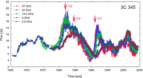
Total flux density light curve of 3C 345 at 4.8, 8, 14.5, 22 and 37 GHz. The data are from the University of Michigan and Metsähovi Radio Observatory monitoring data bases. The arrows mark the times of the ejections of the new jet components C2, C4 and C7.

Open in new tabDownload slide

Figure 3

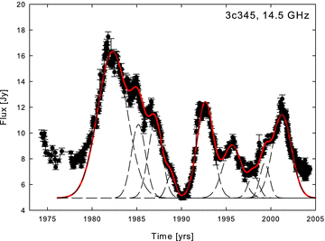
Total flux density light curve of 3C 345 at 14.5 GHz (the data are from the University of Michigan monitoring data base). The long dashed lines show decomposed Gaussian components and the solid line the sum of the fitted Gaussians.

Open in new tabDownload slide

We were able to calculate time-delay core shifts for the epochs of three outbursts associated with the ejection of components for which superluminal speeds have been published: C2, C4 and C7, marked in Fig. 2. Core-shift measurements based on a direct comparison of VLBI images at different frequencies are available for epochs near our measured time delays. Table 2 summarizes and compares the core shifts directly measured from the VLBI images and our calculated core shifts derived from time lags obtained with single-dish observations. The epoch of the VLBI observations and name of the ejected jet components used for the analysis are listed in this table as well.

Biretta, Moore & Cohen (1986) measured core shifts for 3C 345 of 0.05 ± 0.13 mas between 10.7 and 5 GHz in 1982 and 0.111 ± 0.007 mas between 22.2 and 10.7 GHz in 1983.5, during two powerful flares that were associated with the ejection of the new jet components C2 and C4 (Fig. 2).

Component C2 displayed a proper motion of μ = 0.48 ± 0.02 mas yr⁻¹ (Biretta et al. 1986); similar values were detected for this component by Zensus et al. (1995), μ = 0.4–0.53 mas yr⁻¹. The measured time lag between 5 and 8 GHz for the 1982 outburst corresponding to the ejection of C2 is 0.12 ± 0.04 yr. Following our method of calculating the core shifts from the time lags as ΔR_proj (mas) =Δt(ν)_obs (yr) μ (mas yr⁻¹), this corresponds to a core shift of 0.06 ± 0.02 mas. This ‘time-lag’ core shift coincides well with the core shift of 0.05 ± 0.13 mas measured directly by aligning VLBI images (Biretta et al. 1986).

The jet component C4 displayed a proper motion of 0.225 ± 0.015 mas yr⁻¹ (Caproni & Abraham 2004a). Zensus et al. (1995) and Biretta et al. (1986) detected similar values of 0.32 ± 0.15 and 0.295 ± 0.009 mas yr⁻¹ for this jet component. The calculated time lag between 22 and 8 GHz for the 1984 flare is 0.45 ± 0.08 yr. If we use an average of the three proper motions, this yields a time-delay core shift of 0.12 ± 0.02 mas, which is very close to the core shift of 0.111 ± 0.007 mas directly measured by Biretta et al. (1986).

Lobanov (1998) measured core shifts of Δr = 0.05 ± 0.03 mas (5.0–8.4 GHz), Δr = 0.21 ± 0.06 mas (8.4 –22.2 GHz) and Δr = 0.33 ± 0.10 mas (5–22.2 GHz) in ∼1993 (see Table 2). We calculated core shifts using our measured time lags for the flare in 1992: 0.43 ± 0.01 yr (4.8–8.0 GHz); 0.89 ± 0.03 yr (8.0–22.2 GHz) and 1.32 ± 0.03 yr (4.8–22.0 GHz). The proper motion of the jet component C7 ejected during the 1992 flare has been estimated to be 0.208 ± 0.025 mas yr⁻¹ (Caproni & Abraham 2004b) and 0.30 ± 0.16 mas yr⁻¹ (Ros et al. 2000). Taking this value for the newly ejected jet component C7 and using the measured time lags, we can calculate the frequency-dependent core shifts, shown in Table 2.

Table 2 clearly shows that the core shifts measured from the VLBI observations and calculated using our frequency-dependent time lags, and the measured jet-component proper motions coincide very well. This provides a direct test of the proposed method, and suggests that it can be used to reliably calculate core shifts from total flux density light curves.

5 RESULTS FOR THE QUASAR 3C 345

Looking at equation (3), we expect a plot of the time lags versus frequency to have the form

12

The plots of time lags versus frequency for 3C 345 shows that these do, indeed, follow such a power law, enabling us to fit the time lags and derive k_r values from the fits. Fig. 4 shows the fit for flare E as an example. The estimated k_r value from this plot is 1.91 ± 0.04. We used the highest frequency, 37 GHz, as the reference frequency for all measured time lags. Measuring k_r can tell us about the jet geometry, since the distance from the VLBI core to the base of the jet (or, more precisely, the vertex of the cone formed by the jet) scales with k_r as (equation 9). The k_r values contain information about the distributions of the magnetic field and electron number density, since k_r depends on the indices m and n (equation 5), which indicate how the electron number density and magnetic field decrease along the jet (equation 8). The calculated k_r values for each flare of 3C 345 are listed in the last column of Table 1. The range of our k_r values encompasses the average value k_r = 0.96 derived for 3C 345 by Lobanov (1998). We can also use k_r to calculate the core-region magnetic fields using equations (7), (10) and (11). Our k_r values imply magnetic fields in the 5–22 GHz core of 3C 345 ≃ 0.1 G.

Figure 4

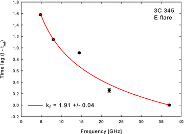
3C 345: plot of time lag measurements versus frequency, using 37 GHz as the reference frequency. The solid curve shows the best-fitting line with a = 5.47 ± 0.04 and k_r = 1.91 ± 0.04.

Open in new tabDownload slide

The measured k_r values for 3C 345 suggest a significant time evolution. The time delays versus frequency evolve with time. Fig. 5 shows time lags for individual flares. The maximum time lag varies between 0.4 and 1.8 yr. Fig. 6 shows that the k_r values are almost at the same level in the period from 1982 to 1992, about 1.8, then begin to decrease to k_r∼ 0.4 in 1999. In this same period, 1982–1990, 3C 345 experienced a major flare, reaching flux density levels of about 19 Jy (Fig. 2). The lower k_r values seem to correspond to flares with less dramatic amplitudes, suggesting a possible connection between k_r and the flux density level. Fig. 7 shows k_r versus the flux at 14.5 GHz; there is a clear tendency for brighter flares to have higher k_r values, reaching a kind of saturation level of about k_r∼ 1.8 for fluxes higher than 6 Jy at 14.5 GHz.

Figure 5

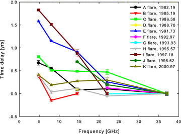
3C 345: time delay of individual events as functions of frequency.

Open in new tabDownload slide

Figure 6

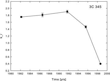
3C 345: time evolution of k_r values.

Open in new tabDownload slide

Figure 7

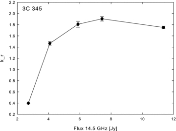
3C 345: correlation between k_r values and amplitude of the flares at 14.5 GHz. The picture shows that the k_r values become higher with higher flux levels.

Open in new tabDownload slide

6 DISCUSSION AND CONCLUSION

We have introduced a new method for calculating core shifts from time lags between the maxima of single-dish flares at different frequencies.

Applying the method to the 3C 345 VLBI jet and integrated light curves from 4.8 to 37 GHz, we found that the directly measured frequency-dependent core shifts and the core shifts calculated with our new method agree very well, supporting the validity of the method and our assumptions. This technique should also be checked using more sources, which we plan to do in a future study.

We have used our method to derive k_r values for 3C 345. We find clear evidence for variability of k_r, with the measured values ranging from 0.4 to 1.9. We find evidence that k_r increases with the core flux level, reaching saturation at a value of ≃1.8 above core fluxes of about 6 Jy. In principle, time evolution of k_r could come about due to changes in the core spectral index, magnetic field distribution or electron number density distribution, since k_r depends on α, m and n (see formula 5). There is no obvious relationship between the value of k_r and the core spectral index (Table 1). Unfortunately, we cannot directly separate the m and n values from the k_r equation (the only exception is if k_r is close to unity, i.e. close to equipartition, in which case it is reasonable to infer m = 1 and n = 2). Therefore, we cannot unambiguously prove that k_r variations are due, for example, purely to variations in α, m or n; it is likely that all three parameters contribute to time variability of k_r. Time variability of k_r values implies that the frequency-dependent core shifts change with time, suggesting that in order to match the astrometric catalogues it is necessary to have simultaneous multifrequency observations.

Using our k_r values, we can estimate the distance of the radio core from the base of the jet, the equipartition magnetic field at 1 pc distance and the equipartition magnetic field in the core (Lobanov 1998; Hirotani 2005). Since not all outbursts are in the equipartition regime as was shown in the previous sections, we have selected for magnetic fields calculations one outburst H with k_r value from a Table 1 closest to unity (and therefore to equipartition regime). We have used intrinsic jet half-opening angle θ = 0°.5 (Jorstad et al. 2005), jet viewing angle φ = 2°.7 (Jorstad et al. 2005), Doppler factor δ = 7.8 (Hovatta et al. 2009) and luminosity distance D_L = 3473 Mpc. Table 3 shows calculated frequency-dependent core shifts, distances between the radio core and the base of the jet, magnetic field at 1 pc and magnetic field in the core for individual pairs of frequencies. We have not used 8-GHz data in the analysis, since the frequency-dependent time lag for the 8/37 GHz pair of frequencies is not very reliable. In error analysis we took into account only the errors in time lags measurements and observed proper motions of jet components. The average magnetic field in the core of 3C 345 at 5–22 GHz is B_core = 0.07 ± 0.02 G and magnetic field at 1 pc is B_1pc = 0.45 ± 0.09 G.

By calculating the frequency-dependent core shifts from the frequency-dependent time delays measured for integrated light curves, we can study the long-term evolution of the core shifts and calculate the core shifts for any particular time when long-term radio light curves are available. Since the total flux density light curves covering more than 30 yr are available for dozens of radio sources, this makes it possible, in principle, to calculate the core-shift evolution over more than 30 yr without constructing and aligning VLBI maps at multiple frequencies. The only input needed from direct VLBI observations is the proper motions of jet components (which can be measured from a series of observations at a single frequency).

NAK was supported for this research through a stipend from the International Max Planck Research School (IMPRS) for Radio and Infrared Astronomy at the Universities of Bonn and Cologne. We would like to thank Shane O’Sullivan for useful discussions. This publication has emanated from research conducted with the financial support of Science Foundation Ireland. The UMRAO has been supported from the series of grants from the NSF and NASA and from the University of Michigan. We thank the referee for his or her prompt review, and comments and suggestions that have significantly improved this paper.

REFERENCES