


Abstract
The first large-scale quantum mechanical simulations of pulsar glitches are presented, using a Gross–Pitaevskii model of the crust-superfluid system in the presence of pinning. Power-law distributions of simulated glitch sizes are obtained, in accord with astronomical observations, with exponents ranging from −0.55 to −1.26. Examples of large-scale simulations, containing ∼200 vortices, reveal that these statistics persist in the many-vortex limit. Waiting-time distributions are also constructed. These and other statistics support the hypothesis that catastrophic unpinning mediated by collective vortex motion produces glitches; indeed, such collective events are seen in time-lapse movies of superfluid density. Three principal trends are observed. (1) The glitch rate scales proportional to the electromagnetic spin-down torque. (2) A strong positive correlation is found between the strength of vortex pinning and mean glitch size. (3) The spin-down dynamics depend less on the pinning site abundance once the latter exceeds one site per vortex, suggesting that unpinned vortices travel a distance comparable to the intervortex spacing before repinning.
1 INTRODUCTION
Glitches are discrete, randomly timed jumps in the famously predictable angular velocity of a pulsar. The statistical distributions of glitches in individual pulsars (power-law sizes and exponential waiting times) point to an underlying threshold-triggered collective process (Melatos, Peralta & Wyithe 2008), akin to grain avalanches in sand piles (Wiesenfeld, Tang & Bak 1989; Morley & Schmidt 1996) or vortex avalanches in type II superconductors (Field et al. 1995). In pulsars, the ‘grains’ are quantized superfluid vortices. A comprehensive theory of why ≳107 (out of ∼1018) vortices simultaneously unpin and self-reorganize to create a glitch remains elusive. A complete solution relies on connecting the microscopic (fm-scale) and macroscopic (km-scale) dynamics of the neutron superfluid in the pulsar interior. The challenge presented by this disparity of scales, especially in replicating collective phenomena, has proved formidable.
In this paper, we present the first comprehensive quantum mechanical simulations of pulsar glitches, using the Gross–Pitaevskii equation (GPE) to model the temporal evolution of the superfluid inside a pulsar. The GPE is a standard tool in condensed matter physics for investigating vortex dynamics in quantum condensates (Pethick & Smith 2002). Our simulations are unique in four ways: (1) the system is much larger than those routinely simulated in condensed matter applications (e.g. Tsubota, Kasamatsu & Ueda 2002; Penckwitt 2003; Tsubota, Kasamatsu & Kobayashi 2010), and therefore contains many more vortices; (2) in addition to the confining potential, we include a grid of pinning sites to model nuclear lattice defects in the pulsar’s crust (Jones 1998b; Donati & Pizzochero 2004, 2006; Avogadro et al. 2007, 2008; Barranco, Broglia & Vigezzi 2010); (3) the container and superfluid are coupled via a feedback torque and (4) we allow the angular velocity of the container to change non-adiabatically. Thus, the simulations describe scales ranging from individual vortex cores to the collective behaviour of several hundred vortices in the presence of a large grid of pinning sites. The results build on previous GPE studies of the general problem of spasmodic superfluid spin-down (Warszawski & Melatos 2010a) and the microphysics of individual vortex unpinning, including knock-on processes involving acoustic radiation and the proximity effect (Warszawski & Melatos 2010b).
The paper is structured as follows. Section 2 summarizes the vortex unpinning paradigm of pulsar glitches, the main features of the numerical model and the feedback mechanism. In Section 3 we describe our algorithm for extracting glitches from simulated spin-down curves. In Section 4 this algorithm is employed in a canonical example. In Section 5 we construct glitch size and waiting-time distributions from relatively small-scale simulations (∼30 vortices) for different pinning parameters. In Section 6, we vary the inertia of the star and the electromagnetic spin-down torque. Section 7 reports results from larger scale simulations involving ∼200 vortices, in which we look for evidence of collective dynamics. Parameter studies with the larger scale simulation are too expensive computationally at this stage. In Section 8 we synthesize the results and present our conclusions.
2 VORTEX UNPINNING PARADIGM
2.1 Overview
The superfluid in a pulsar is composed of neutron Cooper pairs, which interpenetrate the nuclear lattice in the crust (Migdal 1959). The superfluid attempts to match the rotation of the crust by forming quantized vortices, each carrying a quantum of circulation κ=h/(2m), whose areal density is proportional to the angular velocity of the superfluid. In the absence of pinning, vortices form a hexagonal Abrikosov lattice, causing the superfluid to rotate as a rigid body. In equilibrium, the mean areal density of vortices is nF = 2Ω/κ. In reality, however, vortices pin at or between nuclear lattice sites and/or defects, thus distorting the equilibrium vortex configuration. The extent of distortion depends on the configuration and abundance of pinning centres supplied by the crustal lattice of nuclei. Pinning prevents the superfluid from decelerating smoothly with the crust. Glitches are believed to occur when a large number of vortices simultaneously unpin and move outward to new pinned positions. Indeed, GPE simulations reported in Warszawski & Melatos (2010a) exhibit stick-slip vortex dynamics and resulting glitch-like interruptions to the smooth spin-down of the rotating container. Similar spin-up events were observed in laboratory experiments using rotating containers filled with helium II (Tsakadze & Tsakadze 1980).
We construct a simple, two-dimensional pulsar model comprising a superfluid inside a rotating, decelerating crust, in the presence of a pinning grid that corotates with the crust. We include self-consistent coupling between the superfluid and crust by ensuring that angular momentum is conserved overall.
 . For Nv vortices in an Abrikosov lattice, the Feynman relation approximates (the result is exact in the infinite-vortex limit) the azimuthal component of the superfluid velocity at radius r as vϕ≈κNv/(2πr).
The vortex unpinning paradigm presumes that a catalyst exists to spontaneously unpin between 107 and 1015 vortices during a single glitch, with the range deduced from measurements of glitch sizes. To date, the catalyst has not been identified securely. If vortices unpin independently, the number of unpinning events in any time interval follows Poisson statistics (Hakonen, Avenel & Varoquaux 1998). On its own, a Poisson process does not account for the observed power-law distribution of glitch sizes. Hence, a mechanism is needed which correlates vortices, so that the unpinning rate of a particular vortex increases when another vortex (either nearby or far away) unpins; collective unpinning avalanches are essential to explaining pulsar glitches. In recent GPE simulations, Warszawski & Melatos (2010b) demonstrated two mechanisms – in addition to the growing global velocity shear as the crust spins down – for triggering and sustaining vortex avalanches: (i) acoustic radiation from moving vortices, and (ii) vortex proximity knock-on, as unpinned vortices move past their pinned neighbours.
Acoustic radiation results from the propagation of Kelvin waves on vortices (Vinen 2001), from vortex reconnection (Leadbeater et al. 2001) and due to dissipation by accelerating vortices (Parker et al. 2004; Barenghi et al. 2005). The disturbance in the density field as the sound waves propagate is capable of unpinning weakly pinned vortices. The amplitude of the disturbance is a function of vortex acceleration. Therefore, the strongest acoustic radiation results from the repinning phase, as a vortex spirals in to the new pinning site (Warszawski & Melatos 2010b). When the level of dissipation in the system is high, the acoustic disturbance generated by a repinning vortex is weaker than for a low-dissipation system, and hence it is harder to unpin vortices acoustically.
The second effect, proximity knock-on, occurs when two vortices approach sufficiently closely that the Magnus force on at least one of them exceeds the unpinning threshold. It was found that a ballistic unpinned vortex can unpin a pinned vortex at a larger radius via the proximity effect. The distance of closest approach between the two vortices is inversely proportional to pinning strength (Warszawski & Melatos 2010b).
2.2 Gross–Pitaevskii model
 (with units ℎ/2), where ϕ is the azimuthal angle. V is the sum of the confining potential representing the crust and the pinning potential.
In line with standard practice (Jin et al. 1996; Choi, Morgan & Burnett 1998; Penckwitt, Ballagh & Gardiner 2002; Tsubota et al. 2002; Kasamatsu, Tsubota & Ueda 2003), we include in equation (2) a phenomenological treatment of dissipation, modelled by the term −γ∂ψ/∂t. Its effect is to suppress sound waves, thus reducing the relaxation time-scale of the superfluid and ensuring that the wavefunction can adjust to non-adiabatic changes in Ω due to glitches. On the other hand, as reported in Warszawski & Melatos (2010b), sound waves play an important role in vortex unpinning avalanches, by facilitating knock on. Therefore, one must be careful not to raise γ to the point where it quells the latter effect. An accurate estimate of γ in a pulsar is not available at present.
The dissipationless GPE (γ = 0) models a superfluid at T = 0, which does not contain viscous excited-state components. In contrast, solutions to equation (2) for γ≠ 0 are by definition at non-zero temperature. Penckwitt et al. (2002) attributed dissipation in experiments to atom transfer between the viscous thermal cloud and the condensate. Experiments with Bose–Einstein condensates (Haljan et al. 2001) showed that the thermal cloud also influences vortex nucleation. A self-consistent description of this phenomenon requires additional terms in the GPE (Wouters & Carusotto 2007), which are not included in most studies, including ours. Laboratory experiments claim γ = 0.03 in helium II (Abo-Shaeer, Raman & Ketterle 2002); we use γ = 0.05. The dissipative term drives particle loss from the system, which we correct by adjusting the chemical potential, such that the number of particles remains constant (Kasamatsu et al. 2003; Warszawski & Melatos 2010a).
2.3 Container and pinning potential
Using a fourth-order Runge–Kutta algorithm in time, and a fourth-order finite difference scheme for the spatial derivatives, we solve equation (2) for a superfluid in a rotating potential V, in the frame corotating with the potential.
The parameters of vortex pinning within a pulsar have been studied theoretically in great detail (Blasio & Lazzari 1998; Jones 1998b, 2003; Hirasawa & Shibazaki 2001; Avogadro et al. 2008; Barranco et al. 2010). Of particular interest is the pinning strength, the density of pinning sites and the region within the star where pinning is strongest (the superfluid pairing state changes with depth). The strength of pinning is usually calculated from the energy difference between a vortex sitting atop a column of spherical defects and a vortex positioned interstitially. In general, vortices pin to nuclear sites to minimize the region from which superfluid is excluded (the vortex core is devoid of superfluid). Depending on the superfluid density, however, pinning can also occur interstitially (Pizzochero, Viverit & Broglia 1997; Donati & Pizzochero 2004, 2006; Avogadro et al. 2007; Pizzochero 2007). For a pulsar, the characteristic size of the pinning site (the width of a nucleus) is approximately equal to the superfluid healing length (∼1 fm), which is significantly smaller than the lattice (∼10 fm) and intervortex (∼1012 fm) spacings.
2.4 Feedback torque
 , the expectation value of the operator
  . The response of the crust to these changes is an essential element of any pulsar glitch theory. We employ a simple conservation argument, wherein changes in
  are communicated instantaneously to the crust. In reality, changes in the superfluid flow are communicated to the crust by sound and Kelvin waves along vortex lines (Jones 1998a), but these processes are fast. Given an electromagnetic (EM) spin-down torque, NEM, the angular velocity of the crust, Ω, evolves according to
3 AUTOMATED GLITCH FINDER
Our first task is to define exactly what we mean by a glitch. In practice, glitches in pulsar data are extracted ‘by hand’, by looking for discontinuities in the slope and/or curvature of the pulse phase. Recently, Chukwude & Urama (2010) employed an automated glitch-finding algorithm, based on a least-squares goodness-of-fit parameter, to identify microglitches. Since our simulations provide extremely high time resolution (ΩΔt∼ 10−4 revolutions time-step−1 compared to ΩΔt∼ 105 revolutions time-step−1 for the observations), we resolve the glitch spin-up phase; we can identify glitches directly by looking for spin-up events, rather than resorting to polynomial fitting of the phase residuals. The difference between simulation and astrophysical time-scales is also reflected in which physical processes can be resolved. In our simulations, we track the motion of individual vortices between pinning sites, whereas observed glitches appear as unresolved spin-up events, which likely result from a multigeneration vortex cascade.
For the purposes of this investigation, we employ the following simple algorithm for identifying glitches in Ω(t) curves.
Smooth Ω(t) with a top-hat window function w(t) of width Δtsm, viz. Ωsm(t) =∫t0dt′w(t−t′)Ω(t′).
Calculate ΔΩsm(ti) =Ωsm(ti) −Ωsm(ti− 1) for all discrete time points ti in the simulated range.
Find all ts for which ΔΩsm(ts) > 0. For each ts, find the smallest tg(>ts) such that ΔΩsm(tg) ≥ 0 and ΔΩsm(tg+ 1) < 0 (points A and C in Fig. 1 meet this criterion), and record Ωsm(tg).
Locate the global Ωsm(t) minimum between tg− 1 and tg, occurring at tg, min (point B in Fig. 1). Define glitch size as ΔΩ/Ω=[Ωsm(tg) −Ωsm(tg, min)]/Ω(tg) (the vertical distance between the dashed lines in Fig. 1), and waiting time as Δt=tg−tg− 1 (the horizontal distance between points A and C in Fig. 1).
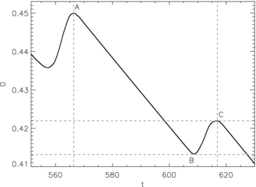
Schematic of how the glitch-finding algorithm operates. A and B mark the positions of the two glitches in the interval 552 < t < 630 on the plot of angular velocity as a function of time Ω(t). The size of glitch C is the difference in Ω between B (the local minimum between A and C) and C (the vertical distance between the horizontal dashed lines). Simulation parameters: V0 = 16.6, η = 1, ΔVi/V0 = 0.0, R = 12.5, Δx = 0.15, Δt = 5 × 10⁻⁴, NEM/Ic = 10−3, Ω(t = 0) = 0.8, npin/nF = 0.97.
The principal weakness of this algorithm is the stipulation in step (iii) that ΔΩsm > 0, which does not capture decreases in  that are smaller than NEMΔt. Depending on the moment of inertia of the crust, ΔΩg due to real glitches may not be greater than the negative ΔΩsm due to the spin-down torque [(NEM/Ic)Δt], and hence this algorithm is not suitable for observational data.
The arrows under the spin-down curve in the top panel of Fig. 2 indicate the positions of glitches found using the above algorithm for a curve smoothed with a top-hat window function of width Δtsm = 0.1. The glitch sizes and waiting times are then used to construct probability density functions (pdfs). In Section 4 we discuss the two bottom panels of Fig. 2, which demonstrate how we subtract a linear fit to the pre-glitch spin-down curve (bottom left-hand panel), and the resulting phase residual curve (bottom right-hand panel).
![Timing signature of a simulated glitch. Top: angular velocity of the crust as a function of time Ω(t) for Ω(t = 0) = 0.8. Ω(t) is smoothed with a top-hat function of width Δtsm = 1.0. The arrows mark the positions of glitches identified using the automated glitch finder described in Section 3. Bottom left: close-up of a glitch at t = 736, bracketed by the dotted rectangle in the top panel. The dotted curve represents the linear model fitted to the pre-glitch spin-down curve. Bottom right: phase residual after removing a pre-glitch linear fit to the interval 710 < t < 730 [Ω(t = 710) = 0.942, ] from the interval 710 < t < 770 shown in the bottom left-hand panel. Simulation parameters: V0 = 16.6, η = 1, ΔVi/V0 = 0.0, R = 12.5, Δx = 0.15, Δt = 5 × 10⁻⁴, NEM/Ic = 10−3, npin/nF = 0.97.](https://oup.silverchair-cdn.com/oup/backfile/Content_public/Journal/mnras/415/2/10.1111/j.1365-2966.2011.18803.x/2/m_mnras0415-1611-f2.jpeg?Expires=1750225221&Signature=Wzg9jZ8aZiw0gh9LrxO3bboZc9QVM8m-FtacJcaUh8oZCLZeZk06B4rs5sieQQqFXuSAeJAsXQpsAVYCWqqqLPHe77D6~tzA4N-GstFJsaFB9NAC1O-SPyQ73w8s9zZtLoTwuALUxanIbLBp5eSBAKEF3FAjPHxJ~hecOjVLA5LTm-9yl68aQ49aUGQwy4wv1hCTahv-Et3QJqQCYSf6LpS~O~mgz6II6YHZA41zdc~aMoXd1fB7a4yZzN6sPM-vXzJkHjQD-J-AvI15iHx2Vf0-ar2Vtr5tYNe48n4XgGLIRUwcHqPzghJRV~xhQQ-5avt91socIkT6xpjRBkzXUQ__&Key-Pair-Id=APKAIE5G5CRDK6RD3PGA)
Timing signature of a simulated glitch. Top: angular velocity of the crust as a function of time Ω(t) for Ω(t = 0) = 0.8. Ω(t) is smoothed with a top-hat function of width Δtsm = 1.0. The arrows mark the positions of glitches identified using the automated glitch finder described in Section 3. Bottom left: close-up of a glitch at t = 736, bracketed by the dotted rectangle in the top panel. The dotted curve represents the linear model fitted to the pre-glitch spin-down curve. Bottom right: phase residual after removing a pre-glitch linear fit to the interval 710 < t < 730 [Ω(t = 710) = 0.942,  ] from the interval 710 < t < 770 shown in the bottom left-hand panel. Simulation parameters: V0 = 16.6, η = 1, ΔVi/V0 = 0.0, R = 12.5, Δx = 0.15, Δt = 5 × 10⁻⁴, NEM/Ic = 10−3, npin/nF = 0.97.
4 CANONICAL GLITCH
Let us now examine a canonical example, which demonstrates the ability of the model in Section 2 to generate astrophysically relevant results. Table 1 lists the set of canonical parameters for this investigation. In the first column, the simulation parameters are given in dimensionless units; their dimensional counterparts are provided in the second column. The third and fourth columns quote the range of values associated with a typical pulsar in dimensionless and dimensional units, respectively.
Dimensionless and dimensional parameters for a typical simulation (second and third columns) and pulsar (fourth and fifth columns). Dimensionless quantities are scaled so as to recover equation (2) from the dimensional form of the GPE, making the replacements described in Section 2 of Warszawski & Melatos (2010a). Pulsar quantities are quoted as a range representative of the pulsar population.
| Quantity | Simulation (dimensionless) | Simulation (dimensional) | Pulsar (dimensionless) | Pulsar (dimensional) |
| R | 12.75 | 10−16 m | 1021 | 104 m |
| V0 | 16.6 | 104 MeV | 10−3 | 100 MeV |
| Ω | 0.8 | 1024 Hz | 10−24–10−21 | 10−1–102 Hz |
| NEM/Ic | 10−3 | 1045 Hz s−1 | 10−63–10−59 | 10−15–10−10 Hz s−1 |
| ttotal | 103 | 10−21 s | 1032–1033 | 108–109 s |
| nF | 0.13 | 2.8 × 10⁻¹⁶ m−2 | 108–1012 | 10−8–10−4 m−2 |
| npin | 0.19 | 2.6 × 10⁻¹⁶ m−2 | 100–104 | 10−14–10−10 m−2 |
| Nv | 30–200 | 30–200 | 1016–1019 | 1016–1019 |
| η | 1 | 1 | 10−6 | 10−6 |
| Δx | 0.15 | 1.5 × 10⁻¹⁶ m | – | – |
| Δt | 5 × 10⁻⁴ | 5 × 10⁻²⁸ m | – | – |
4.1 Set-up
The nuclear lattice of the neutron star inner crust is represented by an 11 × 11 square grid of equal-strength pinning sites (V0 = 16.6, ΔVi/V0 = 0.0), within a box of side length 15, with crust radius R = 12.5 (in dimensionless units). The simulation grid is a 200 × 200 rectangular grid; the grey-scale plots appear circular because |ψ|2 = 0 outside the crust. The time-step and grid spacing are Δt = 5 × 10⁻⁴ and Δx = 0.15, respectively.
The initial conditions are established by accelerating the crust from rest to Ω = 0.8 instantaneously and allowing the system to reach a steady state (defined as when the fractional change in total energy during one time-step drops below 10−5). Once a steady-state solution is obtained, the external spin-down torque NEM( = 10−3Ic) is switched on, and the superfluid-crust system is allowed to evolve.
4.2 Spin-down curve
The spin-down observed after NEM switches on is spasmodic. By watching movies of how the density field |ψ (x, t)|2 evolves, we can easily see why pinning prevents vortices from moving smoothly towards the boundary as the crust decelerates; instead, vortices hop between pinning sites, resulting in step-like decreases in 〈Lz〉. A graph of  versus time is presented in Fig. 3. The positions of glitches identified using the automated glitch-finding algorithm described in Section 3 are marked with arrows. Equation (4) tells us that each step down in
  is accompanied by a step up in Ω (so long as the change in
  exceeds NEMΔt). We see this clearly by comparing the top panel of Figs 2 and 3.
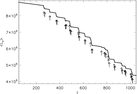
Superfluid angular momentum as a function of time 〈Lz〉(t), in units of ℎ/2, for the canonical spin-down experiment described in Section 4. The arrows indicate the position of glitches identified using the glitch-finding algorithm defined in Section 3. Simulation parameters: η = 1, ΔVi/V0 = 0.0, R = 12.5, Δx = 0.15, Δt = 5 × 10⁻⁴, NEM/Ic = 10−3, Ω(t = 0) = 0.8, npin/nF = 0.97.
A close-up of one of the glitches (bracketed by the dotted rectangle in the top panel of Fig. 2) is shown in the bottom left-hand panel of Fig. 2. Does this look like a pulsar glitch? An important difference is that the spin-down rate before and after the glitch does not change; the Ω(t) curve after the glitch parallels the linear timing model describing the pre-glitch spin-down. This contrasts with some (not all) observed glitches, which frequently produce a permanent increase in the spin-down rate (Wong, Backer & Lyne 2001). The simulation output also lacks a post-glitch recovery phase, during which spin-down is faster than the global average. Given that time-scales associated with the post-glitch recovery phase, i.e. ∼1029ℎ/(n0g) (typically lasting days to weeks; Wong et al. 2001), are associated with coupling of the superfluid to a viscous fluid component not included in these simulations, this result is unsurprising (van Eysden & Melatos 2010). In our simulations, the time for Ω(t) to return to its pre-glitch value is proportional to the size of the glitch and is comparable to the sound crossing of the system, R/cs (Warszawski & Melatos 2010a).
 , has been extracted by performing a least-squares fit of equation (5) to Ω(t) (710 ≤t≤ 730) and is graphed as a dotted curve in the bottom left-hand panel of Fig. 2. The phase residual Δϕ, in units of radians, is therefore
4.3 Statistics
We now construct pdfs of sizes and waiting times using the automated glitch finder. Motivated by the hypothesis that glitches are produced by avalanche dynamics, we look for evidence that the pdfs of sizes and waiting times are distributed as power laws [p(ΔΩg/Ω) ∝ (ΔΩg/Ω)γ] and exponentials [p(Δt) =λ exp (−λΔt)], respectively. Evidence is building that pdfs of this form yield good fits to observational data (Melatos et al. 2008). To fit these functional forms, we find the parameter that minimizes the D statistic (the maximum distance between the cumulative distribution of the model and that of the data). The fit can be rejected with 1 −pKS confidence, where pKS is the Kolmogorov–Smirnov (K–S) probability (Press et al. 1992).
To begin with, we note that the smoothing width Δtsm changes the glitch statistics, as summarized in Table 2. Glitch positions are marked on the spin-down curve in Fig. 4 using arrows for Δtsm = 0.0, 1.0, 5.0 and 10.0 (solid, dotted, dashed and dot–dashed curves, respectively). The curves have been separated vertically for clarity. As Δtsm increases, the number of glitches decreases from Ng = 105 for Δtsm = 0.0 to Ng = 13 for Δtsm = 10.0. The mean waiting time 〈Δt〉 and glitch size 〈ΔΩ/Ω〉 increase five- and ninefold, respectively. The trend in 〈ΔΩ/Ω〉 versus Δtsm is evident in the size pdfs graphed on log–log axes in the left-hand panel of Fig. 5: the pdfs for longer Δtsm are weighted further towards the large-(ΔΩ/Ω) end. Notably, the best-fitting power-law index, γ (we warn the reader that this is not the same quantity as the dissipation parameter γ that appears in equation 2), does not change dramatically with Δtsm; we find γ=−0.994 for Δtsm = 0 (γ can be rejected at the 25.5 per cent confidence level), and γ=−1.104 for Δtsm = 10.0 (rejected at the 5.3 per cent confidence level).
Summary of simulation results for different values of the smoothing width Δtsm[corresponding Ω(t) curves shown in Fig. 4]. Ng is the number of glitches detected, 〈ΔΩ/Ω〉 is the mean glitch size, 〈Δt〉 is the mean waiting time and rp is the Pearson correlation coefficient; rp = 1, −1 and 0 indicate positive, negative and no correlation, respectively. λ is the mean glitch rate that parametrizes the cumulative distribution of waiting times, γ is the power-law index that parametrizes the pdf of glitch sizes. The K–S probability pKS is given in parenthesis; the fit can be rejected at the 1 −pKS confidence level. Simulation parameters: V0 = 16.6, η = 1, ΔVi/V0 = 0.0, R = 12.5, Δx = 0.15, Δt = 5 × 10⁻⁴, NEM/Ic = 10−3, Ω(t = 0) = 0.8, npin/nF = 0.97.
| Δtsm | Ng | 104〈ΔΩ/Ω〉 | 〈Δt〉 | rp | λ (pKS) | γ (pKS) |
| 0.0 | 105 | 51.97 | 7.176 | −0.057 | 0.865(0.000) | −0.994(0.745) |
| 1.0 | 27 | 188.0 | 27.93 | 0.050 | 0.035(0.449) | −0.847(0.613) |
| 5.0 | 16 | 264.9 | 50.51 | 0.428 | 0.016(0.312) | −0.710(0.709) |
| 10.0 | 13 | 253.5 | 62.31 | 0.334 | 0.011(0.130) | −1.104(0.948) |
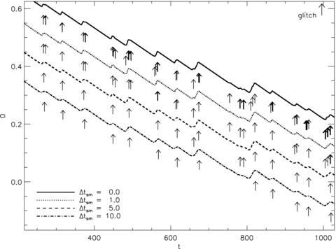
Angular velocity as a function of time Ω(t) for the canonical example described in Section 4, smoothed with a top-hat window function of width Δtsm = 0.0, 1.0, 5.0 and 10 (solid, dotted, dashed, dot–dashed curves, respectively; the curves are shifted vertically down by 0.0, 0.1, 0.2 and 0.3, respectively, to improve visibility). Arrows below each curve mark the positions of glitches found using the glitch-finding algorithm described in Section 3; as Δtsm increases, the number of found glitches decreases. Simulation parameters: V0 = 16.6, η = 1, ΔVi/V0 = 0.0, R = 12.5, Δx = 0.15, Δt = 5 × 10⁻⁴, NEM/Ic = 10−3, Ω(t = 0) = 0.8, npin/nF = 0.97.
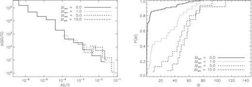
Glitch statistics as a function of the degree of smoothing for the spin-down experiment in Fig. 4. Left: pdf of fractional glitch sizes p(ΔΩ/Ω), binned logarithmically and graphed on log–log axes, for top-hat window functions of width Δtsm = 0.0, 1.0, 5.0 and 10 (solid, dotted, dashed, dot–dashed curves, respectively). Right: cumulative distribution of glitch waiting times P(Δt) for top-hat window functions of width Δtsm = 0.0, 1.0, 5.0 and 10 (solid, dotted, dashed, dot–dashed curves, respectively), graphed on linear axes. Simulation parameters: V0 = 16.6, η = 1, ΔVi/V0 = 0.0, R = 12.5, Δx = 0.15, Δt = 5 × 10⁻⁴, NEM/Ic = 10−3, Ω(t = 0) = 0.8, npin/nF = 0.97.
On the other hand, increasing Δtsm changes markedly the shape of the cumulative waiting-time distribution (right-hand panel of Fig. 5, graphed on linear axes). For Δtsm≤ 1.0, the cumulative probability is dominated by short waiting times (i.e. convex down). For Δtsm≥ 5.0, waiting times are more evenly distributed. Exponential fits to the cumulative probability return mean glitch rates between λ = 0.011 (for Δtsm = 10.0; rejected at the 87 per cent confidence level) and λ = 0.87 (for Δtsm = 0.0; rejected with the near certainty). An exponential functional form for the cumulative distribution for Δtsm = 1.0 is rejected with the least confidence (55.1 per cent).
Glitch positions and distributions depend on Δtsm because smoothing Ω(t) affects the morphology of individual glitches. Understanding this tendency is essential to interpreting observational data properly using our algorithm. For example, increasing Δtsm reduces the size of a glitch, and in some cases erases the glitch altogether. To visualize this, in Fig. 6 we graph an interval of Ω(t) containing an obvious bump (when viewed on the scale graphed in Fig. 4) for different smoothing widths. The arrows in the top panel mark the positions of glitches identified by the automated algorithm for different Δtsm. In the unsmoothed (Δtsm = 0.0, solid) and Δtsm = 1.0 (dotted) curves, we see two obvious bumps at t = 371 and 367.5 (for Δtsm = 0.0 the algorithm finds eight glitches that are not visible by eye on the scale plotted). However, for Δtsm = 5.0 and 10.0, the two bumps merge, and the algorithm finds only one glitch. For Δtsm = 10.0, the glitch is ∼16 per cent smaller than for Δtsm = 5.0. Increased waiting times are a direct corollary of glitches being erased by smoothing.

Close-up of glitches identified using the glitch-finding algorithm described in Section 3, as a function of the degree of smoothing. The plots cover the interval 356 < t < 386 (taken from the Ω curve graphed in Fig. 4). The curves are smoothed with a top-hat window function of width Δtsm = 0.0, 1.0, 5.0 and 10 (solid, dotted, dashed and dot–dashed curves, respectively). The number and position of glitches, shown as arrows in the top panel, changes with Δtsm; for Δtsm≥ 5, one glitch is detected. Simulation parameters: V0 = 16.6, η = 1, ΔVi/V0 = 0.0, R = 12.5, Δx = 0.15, Δt = 5 × 10⁻⁴, NEM/Ic = 10−3, Ω(t = 0) = 0.8, npin/nF = 0.97.
After watching movies of |ψ |2(x, t), we conclude that glitches too small to be discerned by eye on the scale depicted in Fig. 6 are associated with ‘jiggling’, not unpinning. By ‘jiggling’ we mean vortices wobble around their pinning site without unpinning. Multipeaked glitches arise from multistage vortex motion (i.e. one vortex moves, causing a second vortex to move a short time later), precisely the collective avalanche behaviour we are seeking. Observationally, we can only detect pulsar glitches resulting from the motion of many vortices (the smallest observed glitches correspond to ∼107 unpinnings). For this reason, we henceforth adopt Δtsm = 1.0, which also happens to produce the most exponential P(Δt). Thus we retain multipeaked glitches like the one in Fig. 6, whilst excluding glitches not associated with unpinning.
An important recent result from pulsar data analysis is the absence of a reservoir effect: glitch size is uncorrelated with waiting time (Wong et al. 2001; Melatos et al. 2008). In Table 2 we list the Pearson correlation coefficient, rp, relating ΔΩ/Ω and Δt as a function of Δtsm. For Δtsm < 5.0, the two quantities are uncorrelated (rp=−0.057 and 0.050 for Δtsm = 0.0 and 1.0, respectively). For Δtsm≥ 5.0, rp differs significantly from zero (0.428 and 0.334 for Δtsm = 5.0 and 10.0, respectively), suggesting that sizes and waiting times are correlated. The interpretation of this correlation depends on the glitch definition. Since the correlation emerges for smoothing scales that erase multipeaked glitches and ‘jiggling’, it is likely that this correlation exists if the glitch-finding algorithm does not distinguish between single- and multiple-vortex motion. Simulations large enough to house several isolated regions of unpinning activity should not exhibit such a correlation (Melatos et al. 2008).
As observational duty cycles and measurement precision improve, e.g. with the advent of multibeam telescopes, astronomers will begin to resolve the spin-up phase of a glitch, multipeaked glitches and post-glitch oscillations (Kramer & Stappers 2010). Our results suggest that improved measurement precision (equivalent to reducing Δtsm) should lead to a large increase in the number of observed glitches, without altering the shape of the size distribution. For example, reducing Δtsm fivefold doubles the number of glitches. Conversely, the mean glitch rate increases. More speculatively, we also predict that the low-ΔΩ/Ω end of the glitch size pdf is dominated by ongoing, non-collective vortex creep (see Alpar et al. 1984b, for example), likely characterized by a Gaussian cut-off.
5 PINNING PHYSICS
Systematic differences in the pinning strength from pulsar to pulsar may result from different cooling histories (Jones 2001), which alter the morphology and abundance of crystal defects. The role of the pinning strength V0 in glitch physics is crucial. If pinning is weak, vortices spread out smoothly and homologously, allowing the superfluid to decelerate in sympathy with the crust; differential rotation does not build-up in stress reservoirs. On the other hand, if pinning is strong, it may stiffen the vortex lattice to the point where the crust cracks before the vortices are unpinned by the Magnus force (Horowitz & Kadau 2009). Intuitively, we expect that stronger pinning results in larger glitches; either vortices move further once they have unpinned, or more vortices unpin in order to reverse the crust-superfluid shear. In this section we use simulations to test these intuitive relations between glitch distributions and pinning strength.
5.1 Equal pinning potentials
We begin by examining how spin-down depends on V0, in the situation where all the pinning sites are of equal strength (ΔVi = 0). The four grey-scale plots of superfluid density at the top of Fig. 7 are the final states (t = 1025) for simulations with V0 = 0, 8.3, 16.6 and 33.3 (left to right, respectively). Vortices are easily identified as darker spots. The lighter spots represent unoccupied pinning sites. All vortices, except for one in the north-east quadrant of the second panel, are pinned.
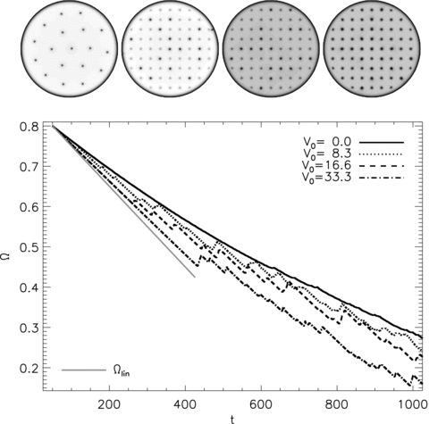
Vortex configurations and spin-down curves for different pinning strengths V0. Top: grey-scale plots of the final (t = 1000) superfluid density for Vi = 0, 8.3, 16.6 and 33.7 (left to right, respectively). The density grey-scale runs from dark (low density) to light (high density). Bottom: angular velocity of the crust as a function of time Ω(t) for Vi = 0, 8.3, 16.6 and 33.7 (solid, dotted, dashed and dot–dashed, respectively). Simulation parameters: η = 1, ΔVi/V0 = 0.0, R = 12.5, Δx = 0.15, Δt = 5 × 10⁻⁴, NEM/Ic = 10−3, Ω(t = 0) = 0.8, npin/nF = 0.97, Δtsm = 1.0.
Without pinning, the vortex lattice expands smoothly and homologously,  decreases smoothly and the superfluid exerts a continuous spin-up torque on the crust via equation (4). The spin-up torque lessens the gradient of Ω (the black curve in Fig. 7) when compared with no feedback, linear spin-down (the solid grey curve). Small bumps in the black curve in Fig. 7 are numerical noise.
 exhibits step-like decreases, accompanied by jumps in Ω, in the dotted, dashed and dot–dashed curves in Fig. 7. The first glitch (at t1) occurs later when the pinning is stronger, viz. t1 = 200 for V0 = 8.3 compared to t1 = 440 for V0 = 33.3. The delay can be understood by considering the velocity shear between pinned vortices and the superfluid in the absence of feedback:
Even in the strongest pinning case, before any unpinning has occurred, the spin-down curve is less steep than Ω(t) =tNEM/Ic (the solid grey curve in Fig. 7). The reason is subtle; it is discussed in detail in Warszawski & Melatos (2010a). While remaining pinned, vortices respond to increasing differential rotation by migrating smoothly to the outer edge of their pinning site. Hence the crust experiences a gradual spin-up torque. Put another way, pinning is not a binary condition; it is weakened gradually as the shear grows.
At the end of the simulation, Ω is highest (Ω = 0.29) for the weakest pinning and lowest (Ω = 0.16) for the strongest pinning, because stronger pinning potentials can sustain greater levels of stress. [Note that this is not the reservoir effect (Link, Epstein & Lattimer 1999; Wong et al. 2001; Melatos et al. 2008), which predicts a correlation between glitch size and waiting time not found in observational data.] In other words, the areal density of remaining vortices after a fixed amount of time is proportional to the pinning strength.
At this point we draw attention to vast discrepancies between typical pulsar parameters and the physical scales modelled by our simulations. The extremely short simulation time (10−21 s in physical units), and the extremely high angular velocity (Ω = 1024 Hz in pulsar units compared to the typical pulsar angular velocity Ω∼ 10 Hz) represent highly non-adiabatic conditions.
5.2 Statistics
Glitch size and waiting-time statistics for different pinning potentials V0 corresponding Ω(t) curves shown in Fig. 7. Ng is the number of glitches detected, 〈ΔΩ/Ω〉 is the mean glitch size, 〈Δt〉 is the mean waiting time and A is the activity parameter. λ is the mean glitch rate that parametrizes the cumulative distribution of waiting times, γ is the power-law index that parametrizes the pdf of glitch sizes. The K–S probability pKS is given in parenthesis; the fit can be rejected at the 1 −pKS confidence level. Simulation parameters: η = 1, ΔVi/V0 = 0.0, R = 12.5, Δx = 0.15, Δt = 5 × 10⁻⁴, NEM/Ic = 10−3, Ω(t = 0) = 0.8, npin/nF = 0.97, Δtsm = 1.0.
| V0 | Ng | 104〈ΔΩ/Ω〉 | 〈Δt〉 | A | γ(pKS) | λ(pKS) |
| 0.0 | 16 | 13.00 | 24.33 | 1.72 | −0.548(0.809) | 0.042(0.895) |
| 8.3 | 48 | 62.90 | 18.01 | 33.85 | −0.818(0.310) | 0.064(0.459) |
| 16.6 | 23 | 187.3 | 31.58 | 28.51 | −0.834(0.762) | 0.029(0.761) |
| 33.3 | 26 | 239.9 | 21.62 | 57.93 | −0.827(0.293) | 0.046(0.474) |
In Fig. 8 we graph logarithmically binned size pdfs on log–log axes. Our glitch-finding algorithm identifies 16, 48, 23 and 26 glitches for V0 = 0, 8.3, 16.6 and 33.3, respectively. The pdfs for simulations with pinning (V0 > 0) exhibit a bias towards larger glitches for larger V0, which also shows up as a ∼fourfold increase in mean glitch size for V0 = 33.3 compared to V0 = 8.3. Power-law fits to the pdfs yield similar indices (listed with the K–S probability in parenthesis in the penultimate column of Table 3) for 8.3 ≤V0≤ 33.3. However, the confidence level with which the fits can be rejected ranges from 23.8 per cent for V0 = 16.6 to 70.7 per cent for V0 = 33.3. We remind the reader that glitches detected in the V0 = 0 case arise from numerical noise, rather than vortex unpinning; this assertion is supported by the small mean glitch size (104〈ΔΩ/Ω〉 = 13.00).
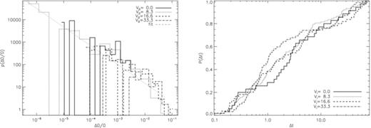
Glitch statistics for different pinning strengths corresponding to the Ω curves graphed in Fig. 7. Left: pdf of fractional glitch sizes p(ΔΩ/Ω) for V0 = 0, 8.3, 16.6 and 33.7 (solid, dotted, dashed and dot–dashed, respectively) logarithmically binned and graphed on log–log axes. The dotted curve is a power-law least-squares fit to the dotted histogram with index −0.818. Right: cumulative probability of glitch waiting times P(Δt) graphed on log-linear axes for V0 = 0, 8.3, 16.6 and 33.7 (solid, dotted, dashed and dot–dashed, respectively). Simulation parameters: η = 1, ΔVi/V0 = 0.0, R = 12.5, Δx = 0.15, Δt = 5 × 10⁻⁴, NEM/Ic = 10−3, Ω(t = 0) = 0.8, npin/nF = 0.97, Δtsm = 1.0.
In the right-hand panel of Fig. 8 we graph cumulative distributions of waiting times for the simulations shown in Fig. 7. Mean glitch rates, λ, derived from exponential fits, are listed in the final column of Table 3. In Melatos et al. (2008), it was found that waiting times for seven of the nine pulsars that have glitched more than six times are well represented by exponential distributions. Taking the results in Fig. 8 all together, we suggest that λ does not depend monotonically on V0 because there is another degree of freedom, 〈ΔΩ/Ω〉, through which the additional stress can be released.
The activity parameter does not appear to scale monotonically with V0. However, A almost doubles between V0 = 8.3 and 33.3. We do not have a physical explanation for this behaviour at this time.
5.3 Pinning site abundance
If pinning occurs at individual nuclei, then ∼109 pinning sites separates neighbouring vortices in a pulsar. Alternatively, if pinning occurs at grain boundaries or along macroscopic faults in the crustal lattice, the ratio of pinning sites to vortices is not necessarily large, and pinning sites may not be evenly spaced. In this section we explore the role of the pinning site density (npin sites per unit area) relative to vortex density (nF = 2Ω/κ vortices per unit area). We present results for simulations with (i) few or no pinning sites, (ii) npin∼nF and (iii) many more pinning sites than vortices. We parametrize the pinning site abundance in terms of the ratio npin/nF in the initial state.
Four pinning scenarios are illustrated in the top panels of Fig. 9 as grey-scale plots of |ψ |2(x, t = 1000) for npin/nF increasing from left to right. The middle panels both correspond to regime (ii). In every panel except the leftmost one (npin/nF = 0.11), all vortices in the final state are pinned. For npin/nF = 0.11, even in the final state, there are only enough pinning sites to pin nine out of 17 vortices (i.e. there are no unoccupied pinning sites). Notably, for npin/nF = 0.11, the vortex lattice is regularly spaced, suggesting that pinning alters the orientation, but not the geometry, of the vortex lattice. For npin/nF = 0.52 and npin/nF = 0.97, vortices are irregularly spaced, as they are forced to adhere to the geometry of the pinning grid. When pinning sites significantly outnumber vortices (right-hand panel, npin/nF = 1.90), the vortex lattice is once again evenly spaced, because enough pinning sites are available for a vortex to ‘choose’ a site near its equilibrium (Abrikosov) position. It should be noted that this equilibrium position changes as the crust spins down.
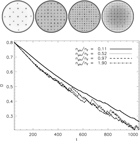
Results from numerical experiments for different pinning abundances npin/nF. Top: grey-scale plots of the final superfluid density for npin/nF = 0.11, 0.52, 0.97 and 1.90 (left to right, respectively). The density scale runs from dark (low density) to light (high density). The faint dots are unoccupied pinning sites; darker dots are pinned vortices. Bottom: angular velocity of the crust as a function of time Ω(t) for npin/nF = 0.11, 0.52, 0.97 and 1.90 (solid, dotted, dashed and dot–dashed, respectively). Simulation parameters: Vi = 16.6, η = 1, ΔVi/V0 = 0.0, R = 12.5, Δx = 0.15, Δt = 5 × 10⁻⁴, NEM/Ic = 10−3, Ω(t = 0) = 0.8, Δtsm = 1.0.
The bottom panel of Fig. 9 graphs the spin-down curves for the four pinning abundances illustrated in the top panels. The example with few pinning sites (npin/nF = 0.11, solid curve) is relatively smooth. Although our algorithm detects 25 glitches, they are small (〈ΔΩ/Ω〉 = 14.84 × 10⁻⁴; cf. 〈ΔΩ/Ω〉 = 13.00 × 10⁻⁴ for V0 = 0) and well separated (〈Δt〉 = 37.10), suggesting that they arise in the rare event that an outwardly moving vortex runs over a pinning site. By contrast, for npin∼nF (dotted, dashed and dash–dotted curves), the spin-down is roughly linear until vortices begin to unpin at t∼ 275, whereupon vortices move towards the edge in spasmodic jumps between pinning sites (vortices do not stop at all pinning sites in their path). For all npin/nF > 0.11, the gradual outward migration of vortices across their pinning sites reduces  , even before vortices have unpinned. For npin/nF = 0.11,
  is considerably less than NEM/Ic for t≳ 50, as the unpinned vortices move smoothly outward almost as soon as the spin-down torque is switched on.
It is physically interesting that the total spin-down of the crust over long time periods is almost identical for npin/nF > 1 and npin/nF∼ 1. The aggregate effect of glitches is insensitive to increases in npin/nF over and above unity. One interpretation is to say that the average distance travelled by a vortex once it unpins is of order n−1/2F, rather than n−1/2pin, so that vortices maintain an approximate Abrikosov lattice, without developing the large-scale spatial inhomogeneities required in self-organized critical avalanche models (Warszawski & Melatos 2008). However, this hypothesis is challenged by three trends. First, the number of glitches and activity parameter increase for npin/nF > 0.11; these qualities scale with n−1/2pin, even though n−1/2F is approximately fixed. Secondly, the mean waiting time is inversely proportional to npin/nF; see Table 4 for details and the right-hand panel of Fig. 9 for cumulative distributions of Δt. Thirdly, the mean glitch size does not change monotonically with npin/nF. Taken together, these results suggest that the typical distance travelled by a vortex in a glitch is a play off between the number of vortices that unpin, the distance to the next available pinning site and the distance the vortex must move to reverse the shear that unpinned it.
Glitch size and waiting-time statistics for different npin/nF[corresponding Ω(t) curves shown in Fig. 7]. Ng is the number of glitches detected, 〈ΔΩ/Ω〉 is the mean glitch size, 〈Δt〉 is the mean waiting time and A is the activity parameter. λ is the mean glitch rate that parametrizes the cumulative distribution of waiting times, γ is the power-law index that parametrizes the pdf of glitch sizes. The K–S probability pKS is given in parenthesis; the fit can be rejected at the 1 −pKS confidence level. Simulation parameters: Vi = 16.6, η = 1, ΔVi/V0 = 0.0, R = 12.5, Δx = 0.15, Δt = 5 × 10⁻⁴, NEM/Ic = 10−3, Ω(t = 0) = 0.8, Δtsm = 1.0.
| npin/nF | Ng | 104〈ΔΩ/Ω〉 | 〈Δt〉 | A | γ(pKS) | λ(pKS) |
| 0.11 | 25 | 14.84 | 37.10 | 2.02 | −0.801(0.911) | 0.053(0.885) |
| 0.52 | 27 | 187.97 | 27.93 | 36.5 | −0.846(0.615) | 0.035(0.450) |
| 0.97 | 48 | 92.41 | 17.36 | 51.5 | −0.875(0.432) | 0.071(0.099) |
| 1.9 | 49 | 111.7 | 15.95 | 68.8 | −0.889(0.312) | 0.068(0.362) |
5.4 Maximum size
Glitch size is governed by the total change in  and hence depends on the number of vortices that unpin, the distance that each vortex travels before repinning and the location from which it unpinned. From the pdfs of ΔΩ/Ω in Fig. 10, we see that the largest glitch is approximately the same for all npin≳nF. If vortex motion is determined by the first encounter with a pinning site, rather than the imperative to reduce shear and maintain equal spacing, then we expect the mean glitch size to scale inversely with the density of pinning sites. This is not observed. By contrast, maximum glitch size does scale monotonically with V0[max(104ΔΩ/Ω) = 36, 538, 1057 and 1641 for V0 = 0, 8.3, 16.6 and 33.3, respectively] because vortices need to move further to reduce the shear sustained by stronger pinning.
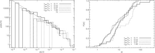
Glitch distributions for spin-down experiments with different pinning abundances npin/nF for the Ω curves graphed in Fig. 9. Left: pdf of fractional glitch sizes p(ΔΩ/Ω) for npin/nF = 0.11, 0.52, 0.97 and 1.90 (solid, dotted, dashed and dot–dashed, respectively) logarithmically binned and graphed on log–log axes. The solid grey curve is a power-law least-squares fit to the solid histogram with index −0.801. Right: cumulative probability of glitch waiting times p(Δt) graphed on log-linear axes for npin/nF = 0.11, 0.52, 0.97 and 1.90 (solid, dotted, dashed and dot–dashed, respectively). Simulation parameters: V0 = 16.6, η = 1, ΔVi/V0 = 0.0, R = 12.5, Δx = 0.15, Δt = 5 × 10⁻⁴, NEM/Ic = 10−3, Ω(t = 0) = 0.8, Δtsm = 1.0.
5.5 Unequal pinning potentials
Pinned vortices at a given radius experience an equal Magnus force. If every pinning site is of equal strength, then vortices at a given radius should unpin simultaneously, yielding periodic glitches of equal size, contrary to observations (Melatos et al. 2008; Melatos & Warszawski 2009). In this section, we investigate the effect of varying the width of the pinning strength distribution ΔVi/V0. The glitch statistics from these simulations are summarized in Table 5.
Glitch size and waiting-time statistics for different ranges of pinning strengths ΔVi/V0[corresponding Ω(t) curves shown in Fig. 11]. Ng is the number of glitches detected, 〈ΔΩ/Ω〉 is the mean glitch size, 〈Δt〉 is the mean waiting time and A is the activity parameter. λ is the mean glitch rate that parametrizes the cumulative distribution of waiting times, γ is the power-law index that parametrizes the pdf of glitch sizes. The K–S probability pKS is given in parenthesis; the fit can be rejected at the 1 −pKS confidence level. Simulation parameters: V0 = 16.6, η = 1, npin/nF, R = 12.5, Δx = 0.15, Δt = 5 × 10⁻⁴, NEM/Ic = 10−3, Ω(t = 0) = 0.8, Δtsm = 1.0.
| ΔVi/V0 | Ng | 104〈ΔΩ/Ω〉 | 〈Δt〉 | A | γ(pKS) | λ(pKS) |
| 0.0 | 28 | 231.2 | 21.72 | 59.82 | −0.818(0.212) | 0.048(0.360) |
| 0.25 | 28 | 173.3 | 22.13 | 44.13 | −0.676(0.596) | 0.043(0.712) |
| 0.5 | 27 | 231.0 | 26.74 | 47.19 | −0.805(0.504) | 0.038(0.232) |
| 0.75 | 24 | 261.8 | 33.42 | 37.80 | −0.776(0.671) | 0.051(0.008) |
| 1.0 | 30 | 206.2 | 26.45 | 47.10 | −0.901(0.253) | 0.070(0.055) |
The spin-down curves in Fig. 11 demonstrate that varying ΔVi/V0 makes little difference to the total spin-down over the time-scale of the simulation; Ω(t = 1000) is approximately the same for all 0 ≤ΔVi/V0≤ 1. However, the timing of the first departure from linear spin-down scales as tg1≈ 1250 + 200(1 −ΔVi/V0). In addition, the glitch statistics change systematically with ΔVi/V0. The pdfs of ΔΩ/Ω graphed in the left-hand panel of Fig. 12 confirm that the minimum glitch size depends on ΔVi/V0, via the minimum pinning strength. The correlation is not strict because the number of draws from the pinning strength distribution is relatively small (11 × 11 = 121), so the minimum Vi does not monotonically scale with ΔVi/V0. We detect no systematic change in the exponent of power-law fits to the size pdf. However, we note that the fits can be rejected with high confidence for ΔVi/V0 = 0 (78.8 per cent) and ΔVi/V0 = 1.0 (74.7 per cent).
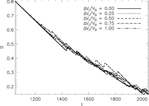
Angular velocity of the crust as a function of time Ω(t) for spin-down experiments with ΔVi/V0 = 0.0, 0.25, 0.5, 0.75 and 1.0 (solid, dotted, dashed, dot–dashed and triple-dot–dashed, respectively). Simulation parameters: V0 = 16.6, η = 1, ΔVi/V0 = 0.0, R = 12.5, Δx = 0.15, Δt = 5 × 10⁻⁴, NEM/Ic = 10−3, Ω(t = 0) = 0.8, Δtsm = 1.0.

Glitch distributions for spin-down experiments with different ΔVi/V0 for the Ω(t) curves graphed in Fig. 11. Left: pdf of fractional glitch sizes (ΔΩ/Ω) for ΔVi/V0 = 0.0, 0.25, 0.5, 0.75 and 1.0 (solid, dotted, dashed, dot–dashed and triple-dot–dashed, respectively) logarithmically binned and graphed on log–log axes. The solid grey curve is a power-law least-squares fit to the solid histogram with index −0.818. Right: cumulative probability of glitch waiting times p(Δt) graphed on log-linear axes for ΔVi/V0 = 0.0, 0.25, 0.5, 0.75 and 1.0 (solid, dotted, dashed, dot–dashed and triple-dot–dashed, respectively). Simulation parameters: V0 = 16.6, η = 1, R = 12.5, Δx = 0.15, Δt = 5 × 10⁻⁴, NEM/Ic = 10−3, Ω(t = 0) = 0.8, Δtsm = 1.0.
Cumulative waiting time distributions are graphed in the right-hand panel of Fig. 12. Exponential fits reveal a tendency for the mean glitch rate to increase with ΔVi/V0 (λ = 0.07 for ΔVi/V0 = 1.0 and 0.043 for ΔVi/V0 = 0.0). This finding disagrees with the uniform pinning scenarios discussed in Sections 5.1 and 5.2, in which λ does not scale inversely with V0.
To interpret the above findings, we suggest that, even for ΔVi/V0 = 0, the effective potential at each pinning site is a function of its departure from an equilibrium position in the Abrikosov lattice. If a vortex is slightly inside or outside (radially) its Feynman position, the effective pinning energy is decreased or increased, respectively, and hence the distribution of pinning strengths can be treated as heterogeneous, even when ΔVi = 0. In a pulsar (npin/nF∼ 1014 if all nuclear sites can pin; see Table 1), the pinned vortices resemble an Abrikosov array. Hence we expect that ΔVi/V0 is more influential in a pulsar than in the simulations presented here.
6 STELLAR PARAMETERS
6.1 Crust moment of inertia
The inertia of the pulsar crust, relative to the inertia of the pinned superfluid, controls the crust’s response to changes in  . Let η=Ic/IS be the ratio of the crust’s moment of inertia, Ic, to the moment of inertia that the superfluid would have if it were a rigid body. If the crust is light (small η), small decreases in
  produce large crustal spin-up events. For sufficiently small η, even vortex creep (Alpar et al. 1984b; Link, Epstein & Baym 1993) should produce small but observable glitches. For larger η, on the other hand, crustal spin-up is smaller. In what follows, we adopt the view proffered by Link et al. (1999) that the ‘crust’ is composed of the rigid nuclear lattice, all charged fluid components that are coupled electromagnetically to the rigid lattice and the unpinned superfluid (which may be a large fraction of the total). Hydrodynamic models of glitch recovery suggest η∼ 1 (van Eysden & Melatos 2010). Results for the numerical experiments presented in this section are summarized in Table 6.
Glitch size and waiting-time statistics for different crustal moments of inertia η[corresponding Ω(t) curves shown in Fig. 13]. Ng is the number of glitches detected, 〈ΔΩ/Ω〉 is the mean glitch size, 〈Δt〉 is the mean waiting time and A is the activity parameter. λ is the mean glitch rate that parametrizes the cumulative distribution of waiting times, γ is the power-law index that parametrizes the pdf of glitch sizes. The K–S probability pKS is given in parenthesis; the fit can be rejected at the 1 −pKS confidence level. Simulation parameters: V0 = 16.6, ΔVi/V0 = 0.0, npin/nF, R = 12.5, Δx = 0.15, Δt = 5 × 10⁻⁴, NEM/Ic = 10−3, Ω(t = 0) = 0.8, Δtsm = 1.0.
| η | Ng | 104〈ΔΩ/Ω〉 | 〈Δt〉 | A | γ(pKS) | λ(pKS) |
| 1.0 | 27 | 188.0 | 27.93 | 36.45 | −0.846(0.615) | 0.035 (0.450) |
| 2.0 | 37 | 74.73 | 25.19 | 22.00 | −0.760(0.916) | 0.065 (0.152) |
| η | Ng | 104〈ΔΩ/Ω〉 | 〈Δt〉 | A | γ(pKS) | λ(pKS) |
| 1.0 | 27 | 188.0 | 27.93 | 36.45 | −0.846(0.615) | 0.035 (0.450) |
| 2.0 | 37 | 74.73 | 25.19 | 22.00 | −0.760(0.916) | 0.065 (0.152) |
As η increases, the mean glitch size diminishes; a given change in  results in a smaller change in Ω. For example, from the spin-down curve in Fig. 13, we see that doubling η halves Ω(t = 1000). Put another way, as η increases, unpinning and outward vortex motion do progressively less to reduce the crust-superfluid shear. Hence, the timing of the unpinning events changes with η. Cumulative waiting time distributions are graphed in the right-hand panel of Fig. 14. They show that the mean waiting time decreases as η increases. The waiting-time distribution is weighted to the low Δt end for η = 2.0 compared to η = 1.0 (e.g. 〈Δt〉 = 27.93, 25.19 and λ = 0.035, 0.065 for η = 1.0, 2.0).
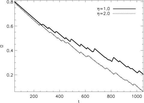
Angular velocity of the crust as a function of time Ω(t) for spin-down experiments with lighter (η = 1) and heavier (η = 2) crusts (solid and dotted curves, respectively). Simulation parameters: V0 = 16.6, ΔVi/V0 = 0.0, R = 12.5, Δx = 0.15, Δt = 5 × 10⁻⁴, NEM/Ic = 10−3, Ω(t = 0) = 0.8, Δtsm = 1.0.
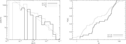
Glitch distributions for spin-down experiments with different ΔVi/V0 for the Ω(t) curves graphed in Fig. 13. Left: pdf of fractional glitch sizes (ΔΩ/Ω) for η = 1 and 2 (solid and dotted curves, respectively) logarithmically binned and graphed on log–log axes. The dotted grey curve is a power-law least-squares fit to the dotted histogram with index −0.846. Right: cumulative pdf of glitch waiting times p(Δt) graphed on log-linear axes for η = 1 and 2 (solid and dotted curves, respectively). Simulation parameters: Vi = 16.6, ΔVi/V0 = 0.0, R = 12.5, Δx = 0.15, Δt = 5 × 10⁻⁴, NEM/Ic = 10−3, Ω(t = 0) = 0.8, Δtsm = 1.0.
The resistance of a heavy crust to spin-up also produces smaller glitches. This result is confirmed by considering the pdf of ΔΩ/Ω for two cases, η = 1.0 and 2.0. Looking at the left-hand panel in Fig. 14, we find that the heavier crust is accompanied by smaller glitches, e.g. 104〈ΔΩ/Ω〉 = 188, 74.73 for η = 1.0, 2.0.
The vertical distance between the curves in Fig. 13 increases with time, demonstrating that the increased glitch rate is not sufficient to compensate for reduced glitch sizes. Over longer time periods than those simulated here,  self-regulates so that the crust-superfluid shear exactly equals the value required to sustain the average unpinning rate leading to
  (given NEM and η). The activity parameter A provides a means of comparing the relative changes in response to the spin-down torque in 〈Δt〉 and 〈ΔΩ/Ω〉; A decreases by ∼33 per cent as η doubles from η = 1.0 to 2.0, demonstrating again that the increased glitch rate does not compensate for the large decrease in glitch size.
6.2 Electromagnetic spin-down torque
The magnetic dipole torque acting on a pulsar ultimately drives the crust-superfluid shear essential to the (un)pinning model of pulsar glitches. Here, we quantify the torque in terms of an electromagnetic spin-down rate, NEM/Ic, in the absence of feedback. The larger the torque, the more quickly Magnus stresses build up in the pinned vortex lattice. Results from simulations in which NEM/Ic is varied are summarized in Table 7.
Glitch size and waiting-time statistics for different NEM/Ic for the Ω(t) curves shown in Fig. 15. Ng is the number of glitches detected, 〈ΔΩ/Ω〉 is the mean glitch size, 〈Δt〉 is the mean waiting time and A is the activity parameter. λ is the mean glitch rate that parametrizes the cumulative distribution of waiting times, γ is the power-law index that parametrizes the pdf of glitch sizes. The K–S probability pKS is given in parenthesis; the fit can be rejected at the 1 −pKS confidence level. Simulation parameters: V0 = 16.6, η = 1, ΔVi/V0 = 0.0, npin/nF, R = 12.5, Δx = 0.15, Δt = 5 × 10⁻⁴, NEM/Ic = 10−3, Ω(t = 0) = 0.8, Δtsm = 1.0.
| NEM/Ic | Ng | 104〈ΔΩ/Ω〉 | 〈Δt〉 | A | Ic〈ΔΩg〉/(〈Δt〉NEM) | γ(pKS) | λ(pKS) |
| 10−4.0 | 3 | 84.28 | 703.4 | 0.0958 | 0.119 | −1.082(0.929) | 0.333 (0.810) |
| 10−3.5 | 39 | 43.68 | 51.42 | 9.52 | 0.269 | −0.720(0.514) | 0.0289 (0.002) |
| 10−3.0 | 27 | 68.50 | 27.93 | 13.28 | 0.245 | −0.819(0.913) | 0.0403 (0.450) |
| 10−2.5 | 84 | 45.39 | 10.44 | 73.98 | 0.137 | −0.984(0.0013) | 0.112 (0.058) |
In Fig. 15 we graph spin-down curves for NEM/Ic = 10−2.5 (solid), 10−3 (dashed), 10−3.5 (dotted) and 10−4 (dot–dash). For NEM/Ic = 10−4.0, we detect few glitches (Ng = 3), owing to the small shear that accumulates over the total lifetime of the simulation [ttotalNEM/Ic = 0.4]. Importantly, the first glitch does not appear at the same value of Ω for different spin-down torques; Ω(t1) = 0.45, 0.46, 0.61 and 0.44 for NEM/Ic = 10−4.0, 10−3.5, 10−3 and 10−2.5, respectively. This result reinforces the findings of hysteresis reported in Jackson & Barenghi (2006) and Warszawski & Melatos (2010a): the spin-down history, not merely the current Ω, determines the number and position of vortices.
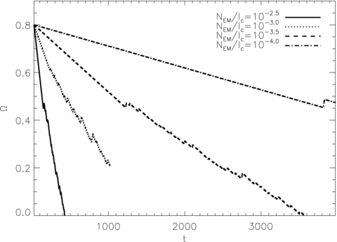
Angular velocity of the crust as a function of time Ω(t) for spin-down experiments with different electromagnetic spin-down torques NEM/Ic=−10−2.5, −10−3.0, −10−3.5 and −10−4.0 (solid, dotted, dashed and dot–dashed curves, respectively). Simulation parameters: V0 = 16.6, η = 1, ΔVi/V0 = 0.0, R = 12.5, Δx = 0.15, Δt = 5 × 10⁻⁴, Ω(t = 0) = 0.8, Δtsm = 1.0.
For a crust-superfluid system with η = 1.0, the observed crust spin-down rate is NEM/(2Ic); see equation (4) with dLz/dt=IcdΩ/dt. For Ng≫ 1, the results in Fig. 15 demonstrate that the fraction of the torque-driven spin-down ttotalNEM/Ic that is reversed by glitches decreases as NEM/Ic increases. Quantitatively, we find Ic〈ΔΩg〉/(〈Δt〉NEM) = 0.269, 0.245 and 0.137 for NEM/Ic = 10−3.5, 10−3.0 and 10−4.0, respectively. We interpret this to mean that weaker torques drive the system adiabatically, allowing the superfluid to match the crust’s deceleration. In a pulsar, the slow spin-down ( ) corresponds to the low-NEM regime. Hence, we can expect on large time-scales the superfluid deceleration matches that of the crust, thus avoiding unfettered growth of differential motion.
Size and waiting-time distributions for NEM/Ic > 10−4.0 are plotted as logarithmically binned pdfs and cumulative probability distributions in the left- and right-hand panels of Fig. 16, respectively. As NEM/Ic increases, one obtains more frequent, smaller glitches. The results reported in Table 7 show that the slopes of power-law fits to the size pdf also increase monotonically with NEM/Ic, as does the rate extracted from exponential fits to waiting-time pdfs (from λ = 0.0289 to 0.112 for NEM/Ic = 10−3.5 and 10−2.5, respectively; since the NEM/Ic = 10−4 curve contains only three glitches, we do not trust the fitted λ). Systematic increases in the activity parameter A (from A = 0.0958 to 73.98 for NEM/Ic = 10−4.0 and 10−2.5, respectively) confirm that increasing NEM/Ic does not trigger the same vortex movements as for smaller NEM/Ic.
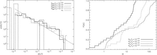
Glitch distributions for spin-down experiments with different electromagnetic spin-down torques NEM/Ic for the Ω(t) curves graphed in Fig. 15. Left: pdf of fractional glitch sizes (ΔΩ/Ω) for NEM/Ic=−10−2.5, −10−3.0, −10−3.5 and −10−4.0 (solid, dotted, dashed and dot–dashed curves, respectively) logarithmically binned and graphed on log–log axes. The solid grey curve is a power-law least-squares fit to the solid histogram with index −0.984. Right: cumulative probability of glitch waiting times p(Δt) graphed on log-linear axes for NEM/Ic=−10−2.5, −10−3.0, −10−3.5 and −10−4.0 (solid, dotted, dashed and dot–dashed curves, respectively). Simulation parameters: V0 = 16.6, η = 1, ΔVi/V0 = 0.0, R = 12.5, Δx = 0.15, Δt = 5 × 10⁻⁴, Ω(t = 0) = 0.8, Δtsm = 1.0.
7 LARGE-SCALE SIMULATIONS
The scale-invariant statistics of pulsar glitches are expected to emerge most clearly in the many-vortex limit. In this section we increase the system size, and hence the vortex number, by an order of magnitude. Prevented by computational expense from undertaking a full parameter study, we present examples of two systems with uniform and variable pinning strengths (ΔVi/V0 = 0.0 and 0.8, respectively), each with ∼200 vortices in total. The simulations ran for ∼2 weeks on a single 2.5-GHz processor. Statistics from the simulations are summarized in Table 8.
Glitch size and waiting-time statistics for different Δtsm and ΔVi/V0[corresponding Ω(t) curves shown in Fig. 18] for large-scale simulations containing ∼200 vortices. Ng is the number of glitches detected, 〈ΔΩ/Ω〉 is the mean glitch size, 〈Δt〉 is the mean waiting time and A is the activity parameter. λ is the mean glitch rate that parametrizes the cumulative distribution of waiting times, γ is the power-law index that parametrizes the pdf of glitch sizes. The K–S probability pKS is given in parenthesis; the fit can be rejected at the 1 −pKS confidence level. Simulation parameters: V0 = 36, η = 1, ΔVi/V0 = 0.0, npin/nF, R = 38, Δx = 0.15, Δt = 5 × 10⁻⁴, NEM/Ic = 10−3, Ω(t = 0) = 0.8.
| Δtsm | ΔVi/V0 | Ng | 104〈ΔΩ/Ω〉 | 〈Δt〉 | A | γ(pKS) | λ(pKS) |
| 0.0 | 0.0 | 4639 | 0.208 | 0.192 | 1007 | −1.26(0.0000) | 1.99(0.000) |
| 0.0 | 0.8 | 196 | 0.500 | 6.25 | 3.14 | −1.08(0.0007) | 0.337(0.000) |
| 0.1 | 0.0 | 491 | 0.752 | 1.55 | 47.65 | −1.23(0.1480) | 1.53(0.000) |
| 0.1 | 0.8 | 139 | 0.591 | 8.81 | 1.87 | −1.05(0.0214) | 0.192(0.0002) |
To maintain the same spatial resolution as in the simulation, we increase the crust radius to R = 38 and impose a 66 × 66 pinning grid (with V0 = 36). We also increase the number of particles in the system 10-fold (via n0), to provide sufficient contrast to distinguish vortices from the background density. We initialize the experiment by instantaneously accelerating the crust from rest to Ω = 0.8 and letting the system reach a steady state. Once a steady state is achieved, the crust is subjected to a spin-down torque NEM = 10−3Ic.
The grey-scale plot in the left-hand panel of Fig. 17 depicts the initial superfluid density for uniform pinning (ΔVi/V0 = 0.0). The two insets zoom in on regions where vortices sit interstitially. The smooth increase in |ψ|2 with radius, indicated by the radial colour gradient, represents the standard parabolic density profile, analogous to the meniscus of a rotating bucket of water (Warszawski & Melatos 2010a). Initially the vortices (dark dots in Fig. 17; light dots are unoccupied pinning sites) are surrounded by a vortex-free corona in the region 4 ≤r≤ 38, highlighting the distortion and hysteresis wrought by the pinning grid (see section IVB of Warszawski & Melatos 2010a). By the end of the simulation, the vortices are approximately evenly distributed across the pinning grid; see the grey-scale plot in the right-hand panel of Fig. 17. The radial density gradient is shallower because Ω is lower than its initial value. We can see that vortices have moved from their initial positions; vortices present in the insets in the left-hand panel of Fig. 17 are absent from the right-hand panel.
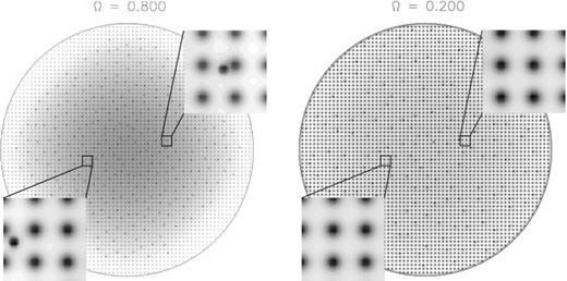
Grey-scale plots of the initial (Ω = 0.8, left) and final (Ω = 0.2, right) superfluid density |ψ|2 for a 600 × 600 simulation with R = 38 and Vi = 36. The insets zoom in on regions with dimensions 3 × 3. Vortices are recognizable as the darker dots, initially clustered towards the centre of the crust and evenly spaced at the end of the simulation. Unpinned vortices can be seen in the initial but not the final insets. Simulation parameters: V0 = 36, η = 1, NEM/Ic = 10−3, R = 38, Δx = 0.15, Δt = 5 × 10⁻⁴, Ω(t = 0) = 0.8, Δtsm = 0.1.
The spin-down curves for ΔVi/V0 = 0.0 and 0.8 (solid and dotted curves in Fig. 18, respectively), smoothed with a top-hat window function of width Δtsm = 0.1, reveal only small glitches (104〈ΔΩg/Ωg〉 = 0.752 and 0.591 for ΔVi/V0 = 0.0 and 0.8, respectively). This result is unsurprising. In larger systems, each vortex corresponds to a smaller fraction of the total angular momentum. To achieve glitches as large as those produced by a R = 12.5 system, ∼10 times more vortices must unpin simultaneously. Dissipation, which suppresses sound waves, renders knock-on events less likely; hence such large-scale collective unpinning is rare in the systems simulated here. The insets show close-ups of the largest glitch (top right and bottom left for ΔVi/V0 = 0.0 and 0.8, respectively). The spin-up phase of the largest glitch in the ΔVi/V0 = 0.0 curve is bumpy. In fact, the vertical distance between the bumps is of order the height of the largest glitch in the ΔVi/V0 = 0.8 curve, which does not exhibit the same ‘bumpiness’.
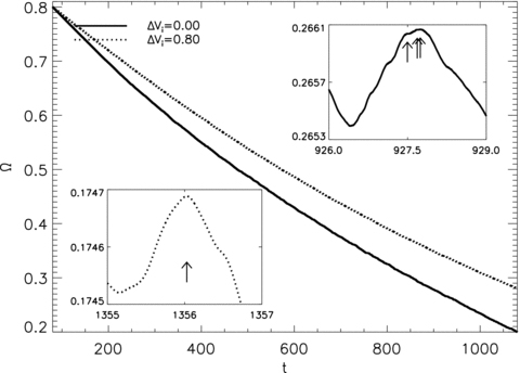
Angular velocity of the crust as a function of time Ω(t) for large-scale spin-down experiments with ΔVi/V0 = 0.0 and 0.8 (solid and dotted curves, respectively). Grey-scale plots of the initial and final superfluid density |ψ|2 for ΔVi/V0 = 0.0 are shown in Fig. 17. Left inset: close-up of glitch at t = 804.3 from ΔVi/V0 = 0.8 curve. Right inset: close-up of glitch at t = 806.1 from ΔVi/V0 = 0.0 curve. Glitch positions are marked as arrows. Simulation parameters: V0 = 36, η = 1, NEM/Ic = 10−3, R = 38, Δx = 0.15, Δt = 5 × 10⁻⁴, Ω(t = 0) = 0.8, Δtsm = 0.1.
Pdfs of ΔΩ/Ω and cumulative distributions of Δt are graphed in the left- and right-hand columns of Fig. 19, respectively; the solid curves are for ΔVi/V0 = 0.0 and the dotted curves are for ΔVi/V0 = 0.8. Since there is an obvious turnover in the size distribution at ΔΩ/Ω≈ 7 × 10⁻⁷, power-law fits are to p(ΔΩ/Ω≥ 7 × 10⁻⁷). The top panels refer to glitches detected in the unsmoothed Ω curve, whereas the bottom panels are smoothed with Δtsm = 0.1. For both values of ΔVi/V0, smoothing flattens the size distribution. Comparison with Fig. 8 reveals that the smallest glitch in the larger system is six times smaller than the smallest glitches for the R = 12.5 systems discussed in previous sections, which agrees with the ∼sixfold increase in vortex number Nv. If a single vortex is responsible for the smallest glitch, then the size of the smallest glitch should scale inversely with Nv. For Δtsm = 0.1, the fitted power law is marginally shallower for ΔVi/V0 = 0.8 (γ=−1.05) than for ΔVi/V0 = 0.0 (γ=−1.23).
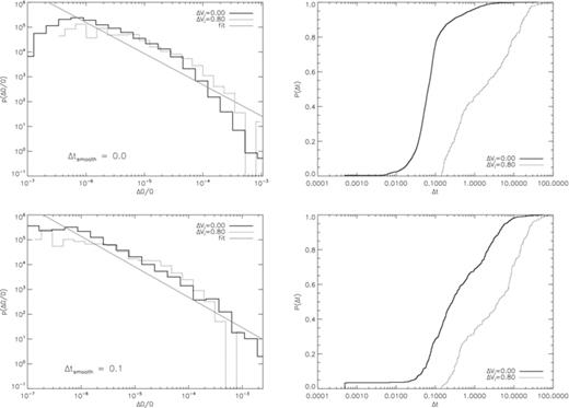
Left: pdf of fractional glitch sizes (ΔΩ/Ω) for the Ω(t) curves graphed in Fig. 18 for ΔVi/V0 = 0.0 and 0.8 (solid and dotted curves, respectively) unsmoothed (top) and smoothed with top-hat window function of width Δtsm = 0.1 (bottom), logarithmically binned and graphed on log–log axes. The solid grey curves are power-law least-squares fits to the solid histograms for ΔΩ/Ω≥ 7 × 10⁻⁷, with indices −1.26 and −1.23, respectively. Right: cumulative pdf of glitch waiting times p(Δt) graphed on log-linear axes with ΔVi/V0 = 0.0 and 0.8 (solid and dotted curves, respectively) unsmoothed (top) and smoothed with top-hat window function of width Δtsm = 0.1 (bottom). Simulation parameters: V0 = 36, η = 1, NEM/Ic = 10−3, R = 38, Δx = 0.15, Δt = 5 × 10⁻⁴, Ω(t = 0) = 0.8, Δtsm = 0.1.
The waiting times tend to lengthen as ΔVi/V0 increases, as observed in smaller systems (see Fig. 12). For ΔVi/V0 = 0.0, smoothing broadens the waiting-time distribution significantly. The top right-hand panel of Fig. 12 reveals a strong periodicity at Δt≈ 0.05 in the waiting-time distribution for Δtsm = 0.0. This may be evidence of the periodic glitches expected from a system in which stress increases over time by the same amount on vortices pinned with equal strength. Despite the overall slower spin-down for ΔVi/V0 = 0.8 (cf. Fig. 18), the longer waiting times are not matched by larger glitches. This is likely due to one of two reasons: (i) much of the crust-superfluid shear is reversed by smooth vortex motion, unhindered by weak pinning or (ii) glitches are too small to cause a bump (positive change) in Ω, and hence are not detected by our glitch-finding algorithm.
Two significant differences between this experiment and those described in Sections 4–6 prevent us from attributing the altered spin-down behaviour (smaller glitches) entirely to system size. First, the ratio of pinning sites to vortices is significantly higher (npin/nF≈ 5) in this experiment than in the smaller systems, whilst the spacing of the pinning sites, relative to the vortex core size, is smaller. It may be that such a closely spaced pinning grid presents the vortices with a nearly homogeneous, elevated potential, effectively weakening the pinning strength. Secondly, since the Magnus force on pinned vortices is proportional to |v−vs | ≈r(〈Lz〉/Is−Ω) at the pinning site, the larger radii of many of the pinned vortices in the R = 38 system make for larger Magnus forces for smaller values of (〈Lz〉/Is−Ω).
8 DISCUSSION
The numerical experiments described in this paper demonstrate from first principles that a superfluid coupled to its container via vortex pinning spins down spasmodically. The experiments are designed to explore how the distributions of pulsar glitch sizes and waiting times depend on pinning and stellar parameters. Computational limitations prevent us from probing the parameter regime most appropriate to the pulsar glitch problem. However, we do our best to mimic astrophysical conditions by adopting the same ordering of dimensionless parameters as in nature. Qualitatively, and with respect to the canonical parameters listed in Table 1, the pulsar problem involves weak (but still effective) pinning, slow electromagnetic spin-down, a huge number of vortices, an even larger number of pinning sites and a heavy crust.
In order to speed up the process of compiling glitch statistics and minimize its subjective element, we devise an automated glitch finder. Since the glitch-finding algorithm identifies all positive jumps in ΔΩ, it is necessary to smooth Ω so as to filter out post-glitch oscillations or numerical noise. In the future, improvements in timing and observational duty cycle should allow real pulsar spin-down curves to be analysed in the same way.
Our simulations lend new insights into aspects of the physics of pulsar glitches.
Stronger pinning causes larger glitches, with 〈ΔΩg/Ω〉≈ 7.6Vi. This is not as obvious as it may sound. Prima facie it is equally likely that strong pinning leads to a large average shear with small, frequent fluctuations. In fact, this does not happen.
When pinning sites and vortices are equally numerous, vortices conform to the geometry of the pinning grid, producing larger glitches than if pinning sites are more abundant than vortices. Waiting times are also longer for npin∼nF than for npin > nF.
Glitch sizes are insensitive to increases in the pinning site abundance beyond parity (i.e. nF∼npin), because vortices move across many pinning sites to negate the local shear, rather than stopping at an adjacent pinning site. The distance travelled by an unpinned vortex is a key input to heuristic glitch models (e.g. Warszawski & Melatos 2008; Melatos & Warszawski 2009).
A broader range of Vi results in a broader range of glitch sizes and more frequent glitches.
A heavier crust produces more large glitches and longer waiting times than does a lighter crust.
A strong spin-down torque catalyzes smaller, more frequent glitches than a weak torque.
Pulsar astronomers derive the strength of the pulsar magnetic field from the spin-down rate of the crust without allowing for superfluid feedback. The results in this paper demonstrate that this is inaccurate. Even when no vortices have yet unpinned (e.g. t≤ 430 in the dot–dashed curve in Fig. 7),
 is a function of both the external torque and the superfluid dynamics (via equation 4). As vortices migrate towards the edge of their pinning sites, the smooth, internal spin-up torque effectively reduces the crust’s spin-down rate. However, this effect is much smaller in a real pulsar than in our simulations. For example, if all vortices move radially outward by the width of a nucleus,
  . A larger, smooth spin-up torque results from homogeneous outward vortex creep.
Table 9 summarizes how measures of glitch activity, like the mean size and waiting time and the glitch activity parameter, depend on the underlying physical levers, like the pinning strength/abundance and the electromagnetic torque. A dot indicates where there is no/weak dependence; a plus (minus) sign indicates that the measure of activity increases (decreases) as the physical variable increases. Intuitively, we expect that a positive correlation with mean glitch size is accompanied by a positive correlation with mean waiting time. For V0, for example, this is not the case; mean glitch size increases with increasing V0, whereas mean waiting time does not change monotonically with V0. One possible explanation is that the simulation has not run long enough to establish a critical velocity shear that ensures a net outward flux of vortices that matches the superfluid spin-down to that of the crust (Alpar et al. 1984a; Melatos & Warszawski 2009). The increasing vertical distance between the spin-down curves in Fig. 7 confirms that this critical shear has not yet been established.
Summary of how simulated glitch statistics depend on the physical levers of the model. A plus (minus) sign indicates that the quantity in the left column increases (decreases) when the parameter in the column heading increases. A dot indicates no clear correlation.
| Quantity | Δtsm | V0 | ΔVi/V0 | npin/nF | η | NEM |
| 〈ΔΩ/Ω〉 | + | + | . | . | − | . |
| 〈Δt〉 | + | . | + | − | − | − |
| A | . | + | . | + | − | + |
| Quantity | Δtsm | V0 | ΔVi/V0 | npin/nF | η | NEM |
| 〈ΔΩ/Ω〉 | + | + | . | . | − | . |
| 〈Δt〉 | + | . | + | − | − | − |
| A | . | + | . | + | − | + |
If pinning is not strong at the densities where only a neutron superfluid is present (Donati & Pizzochero 2003 show that V0 depends on density), then glitches may arise from the physics of the outer pulsar core, where the neutron superfluid co-exists with a superconducting proton fluid. Magnetic flux tubes in the superconducting fluid complicate the superfluid vortex dynamics, rendering the simple Magnus-force dynamics in this paper invalid. Hence, simulations presented in this paper are relevant only to the pulsar inner crust, whose density lies in the range 1011≲ρ≲ 1014 g cm−3, where the majority of protons are confined within nuclei (Pethick et al. 2000).
The discrete Ω jumps in the spin-down curves graphed throughout this paper are analogous to the step changes in magnetic field seen in fig. 1 of Field et al. (1995), caused by magnetic flux tube avalanches in type II superconductors. Superconductor experiments exhibit power-law size distributions over two decades, with exponents ranging from −1.4 to −2.2. Several authors have successfully modelled the superconducting system as a self-organized critical system fluctuating about a Bean state, governed by collective unpinning and motion of flux tubes (Bassler & Paczuski 1998). A natural theoretical framework for a self-organized critical system with knock-on mechanisms is a branching process. The characteristic power-law index of such systems is −1.5 (Carreras et al. 2002), consistently steeper than the size distributions reported in this paper. We therefore conclude that either (i) we are not simulating a self-organized critical system or (ii) our definition of event size and/or identification algorithm is not correct.
Although our glitch size distributions are not inconsistent with power laws, we do not find conclusive evidence of collective vortex behaviour, e.g. many-generation cascades of unpinning events in movies of |ψ|2. This is not surprising. Warszawski & Melatos (2010b) found that sound waves from moving vortices unpin nearby vortices only when dissipation is low. In this paper’s experiments, for computational expediency, we use γ = 0.05, whereas Warszawski & Melatos (2010b) required γ = 0.0025 to facilitate an acoustic knock-on event given the same characteristic pinning strengths as studied in this paper. In contrast, the proximity knock-on mechanism identified by Warszawski & Melatos (2010b) does occur in the simulations presented here. Hence collective dynamics are not excluded completely.
Collective effects emerge most fully in large systems. We therefore present preliminary results from large, computationally expensive simulations with ∼200 vortices. The large simulations yield a broader range of glitch sizes than smaller systems. Power-law fits to the entire size distribution can be rejected with high confidence. Imposing a minimum cut-off, to create a subset of larger glitches, yields a distribution that can be fitted by a power law that is rejected with less confidence. Physically, this may be equivalent to distinguishing between creep-like vortex motion and avalanche events.
In addition to requiring larger system sizes, reliable pulsar glitch simulations must also address the role of pinning along the length of a vortex. When a three-dimensional vortex moves radially outward, it either ‘unzips’ from pinning sites along its length or moves in small vertical segments that behave effectively as individual vortices. Three dimensions also introduce the possibility of turbulent superflow, i.e. a polarized vortex tangle (Schwarz 1988; Barenghi et al. 2001; Kobayashi & Tsubota 2007; Mongiovì & Jou 2007). Tangled vortices can form bundles, which behave as multiply quantized vortices. A full understanding requires further investigation using 3D simulations.
Finally, as well as expanding GPE simulations to larger systems and higher resolution, we recommend that progress in understanding pulsar glitches can be achieved via cellular automata (Morley & Schmidt 1996; Bassler & Paczuski 1998; Warszawski & Melatos 2008). The generic behaviour observed in GPE simulations can be used to devise microscopic rules for such automata.
We thank Dr Andrew Martin and Dr Natalia Berloff for enlightening discussions on many of the topics addressed in this paper. LW acknowledges the support of an Australian Postgraduate Award.
REFERENCES
