


Abstract
We present here photometric redshift confirmation of the presence of large-scale structure around the z= 1.82 quasi-stellar object (QSO) RX J0941, which shows an overdensity of submillimetre (submm) sources. Radio imaging confirms the presence of the submm sources and pinpoints their likely optical near-infrared (NIR) counterparts. Four of the five submm sources present in this field (including the QSO) have counterparts with redshifts compatible with z= 1.82. We show that our photometric redshifts are robust against the use of different spectral templates. We have measured the galaxy stellar mass of the submm galaxies from their rest-frame K-band luminosity obtaining log(M*/M⊙) ∼ 11.5 ± 0.2, slightly larger than the Schechter mass of present-day galaxies, and hence indicating that most of the stellar mass is already formed. We present optical-to-radio spectral energy distributions (SEDs) of the five Submillimetre Common-User Bolometer Array (SCUBA) sources. The emission of RX J0941 is dominated by reprocessed active galactic nucleus (AGN) emission in the observed mid-IR (MIR) range, while the starburst contribution completely dominates in the submm range. The SEDs of the other three counterparts are compatible with a dominant starburst contribution above ∼24 μm, with star formation rates ∼2000 M⊙ yr−1, central dust masses log(Mdust/M⊙) ∼ 9 ± 0.5 and hence central gas masses log(Mgas/M⊙) ∼ 10.7. There is very little room for an AGN contribution. From X-ray upper limits and the observed 24 μm flux, we derive a maximum 2–10 keV X-ray luminosity of 1044 erg s−1 for any putative AGN, even if they are heavily obscured. This in turn points to relatively small black holes with log(M•/M⊙) ≲ 8 and hence stellar-to-black hole mass ratios about 1 order of magnitude higher than those observed in the present Universe: most of their central black hole masses are still to be accreted. Local stellar-to-black hole mass ratios can be reached if ∼1.3 per cent of the available nuclear gas mass is accreted.
1 INTRODUCTION
It is currently commonly accepted that structures in the Universe are formed through hierarchical processes, in which smaller structures collapse to form galaxies, which then group together or coalesce to form larger galaxies and galaxy groups and clusters. Within this general background, ‘antihierarchical’ behaviour has been observed, in the sense of the most dense large-galaxy-size structures collapsing earlier and evolving faster than smaller galaxies (e.g. Renzini 2006, and references therein). These processes are thought to be accompanied by channelling of material to the central regions, where it forms stars and feeds a growing black hole (BH). The feedback of the latter regulates galaxy formation in an ‘evolutionary sequence’ (e.g. Silk & Rees 1998; Fabian 1999; Granato et al. 2004; Page et al. 2004; Di Matteo, Springel & Hernquist 2005; King 2005; Stevens et al. 2005). According to these models, galaxies grow through star formation and at first host ‘small’ BHs possibly in very dense and obscured nuclear environments. As time progresses, the combined radiative and mechanical output from star formation and the BH accretion grows too, until the active galactic nucleus (AGN) reaches quasi-stellar object (QSO) luminosities and literally blows away the circumnuclear material. This effectively terminates star formation, and the supermassive BH (SMBH) shines briefly (in cosmic terms) as an unobscured QSO. Once it has accreted the remaining material, the QSO switches off, leaving a passively evolving galaxy with a ‘dormant’ SMBH, such as those observed in present-day massive galaxies (Marconi & Hunt 2003).
The far-infrared (FIR)–submillimetre (submm) spectral region is ideally suited for searching for star formation, since the blackbody-like (grey body) emission by cold dust associated with star formation peaks at those wavelengths. At the same time, it suffers very modest obscuration from the circumnuclear material. This is proved by the large numbers of strongly star-forming submm galaxies (SMGs) detected by Submillimetre Common-User Bolometer Array (SCUBA), AzTEC, Submillimetre Array (SMA) and, lately, Herschel, among other facilities.
There are many multi-wavelength studies of SMGs, both from surveys in ‘blank fields’ (e.g. Smail, Ivison & Blain 1997; Hughes et al. 1998; Eales et al. 1999; Scott et al. 2002; Alexander et al. 2005; Borys et al. 2005; Coppin et al. 2006; Laird et al. 2010) and targeting overdensities of such sources around high-redshift objects (e.g. Ivison et al. 2000; Kurk et al. 2000; Pentericci et al. 2000; Smail et al. 2003; Stevens et al. 2003, 2004; De Breuck et al. 2004; Greve et al. 2004; Venemans et al. 2007; Priddey, Ivison & Isaak 2008; Chapman et al. 2009). These studies probe the properties of the star formation and the AGN, and the association between both phenomena, although there are not many cases in which this association has been proved. SMGs have substantial stellar masses in place by z∼ 2. A relatively high fraction of SMGs host AGN (e.g. Alexander et al. 2005, but see Laird et al. 2010), which seem to have BH-to-stellar mass ratios smaller than local galaxies (Borys et al. 2005; Alexander et al. 2008). This implies that BH growth lags galaxy growth, since the host galaxies are already mature, while the BHs still require substantial growth (e.g. by about a factor of 6), which, however, can be accommodated within the limits imposed by the lifetime of the submm-bright phase (Alexander et al. 2008), if accretion occurs close to the Eddington limit (Eddington 1913; Rees 1984). The observed population of z∼ 2 SMGs would be sufficient to account for the formation of the population of bright ellipticals seen in the present Universe (Swinbank et al. 2006).
We have found (Page et al. 2004; Stevens et al. 2005) a sample of X-ray-obscured QSOs at z∼ 2 (when most of the star formation and BH growth are occurring in the Universe) with strong submm emission, much higher than X-ray-unobscured QSOs at similar redshifts and luminosities, which, however, represent 85–90 per cent of the X-ray QSOs at that epoch. This submm emission is too high to come from the AGN (Page et al. 2001; Stevens et al. 2005). The fields around these objects show strong overdensities of SMGs (Stevens et al. 2004, 2010, hereafter S10). The ultraviolet (UV) and X-ray spectra of the central QSOs (Page et al. 2011) show evidence for strong ionized winds which produce the X-ray obscuration. Piecing all these clues together, we infer that the host galaxies of these QSOs are undergoing strong star formation rate (SFR), while the central SMBH are also growing through accretion. The ionized winds are strong enough to quench the star formation, so the QSOs must be just emerging from a strongly obscured accretion state to become ‘normal’ unobscured QSOs with passively evolving galaxies, in an evolutionary stage which might last about 10–15 per cent of the QSO lifetime. They appear to be in the centres of high density peaks of the Universe.
In this paper, we endeavour to prove the physical association of one of those overdensities to its central QSO (RX J094144.51+385434.8, henceforth RX J0941). We also investigate the nature and evolutionary stage of those SMGs through their rest-frame UV–FIR spectral energy distributions (SEDs).
The outline of this paper is as follows. In Section 2, we summarize the data used in this paper and the reduction process. In Section 3, we describe how the source catalogues in each band have been merged into a single catalogue and how that catalogue has been used to obtain photometric redshifts. These are then used in Section 4 to show which objects are associated with the structure around the QSO and to the submm sources, and how we have obtained the different physical parameters for each object. The evolutionary stage of our sources is discussed in Section 5. Finally, in Section 6, we summarize our results. We have assumed throughout this paper a Hubble constant H0 = 70 km s−1 Mpc−1 and density parameters Ωm = 0.3 and ΩΛ = 0.7. The spectral index α is defined as Fν∝να.
2 DATA
The R-band, K-band, Spitzer and SCUBA data used here are the same ones discussed in Stevens et al. (2004; S10), but with a new reduction of the R-band data, all the astrometry tied to this band (see below) and fluxes for fainter Spitzer sources. The i-, Z- and J-band, and radio data are newly presented here. We show in Fig. 1 the central area of the submm images along with contours and images of the radio data. The region to the north-west (NW) around source 850_3 is shown in Fig. 5.

Finding charts of a 2.1 × 1.3 arcmin2 region around the submm structure associated with RX J0941 (N is up and E is to the left). The region around 850_3 (to the NW of RX J0941) is shown separately in Fig. 5. Top left-hand panel: 450 μm S/N image with 2σ–6σ contours (in steps of 0.5σ, dashed cyan) and 6 cm 2σ–5σ contours (in steps of 1σ, yellow), the numbers and crosses in cyan correspond to the 450 μm sources in Table 1. Top right-hand panel: 850 μm S/N image with 2σ–8σ contours (in steps of 0.5σ, dashed magenta) and 20 cm 2σ–5σ contours (in steps of 1σ, yellow), the numbers and ‘x’ in magenta correspond to the 850 μm sources in Table 1 (the cyan crosses to the 450 μm sources in that table). Bottom left-hand panel: 6 cm image and contours (as above) with source numbers and crosses as above (note that sources 1 and 2 are common to 450 and 850 μm). Bottom right-hand panel: 20 cm image and contours (as above) with source numbers and markers as above. In grey-scale, magenta appears slightly darker than cyan and the steeper yellow contours appear white.
Finding charts for 850_3. Same layout as in Fig. 3.
We give in Table 1 the deboosted 850 and 450 μm fluxes from S10, where we have symmetrized the error bars taking the worst of the upper and lower error bars. The source extraction method used in S10 (described in Scott et al. 2002) can miss real sources separated by less than a beam (14.2 arcsec for 850 μm). This is probably the case for 450_3, which is blended together with 850_2 (see Fig. 1 and S10): in 850 μm these two sources are part of an almost north–south (NS) structure with 850_2/450_2 in the southern tip and 450_3 close to the northern tip.
SCUBA source positions and fluxes (see Section 2). The first part of the table corresponds to 850 μm and the second to 450 μm. Our source number for the counterpart is given under # (see Table 3 and Section 4.2), the best-fitting photometric redshift under zp and its confidence interval under 1σ. SFRs and 8–1000 μm IR luminosities are from template SEDs (see Section 4.2). Dust mass ranges and galaxy stellar masses are derived in Sections 4.4 and 4.5, respectively. IR luminosities, SFR, dust masses and galaxy stellar masses are obtained assuming z = 1.82.
| Source | RA (h m s) | Dec. (° ‴) | Flux (mJy) | # | zp | 1σ | L8−1000 μm (1013 L⊙) | SFR (M⊙ yr−1) | Mdust (108 M⊙) | log M*a (log M⊙) |
| 850_1b | 09 41 44.63 | +38 54 38.88 | 12.4 ± 1.1 | 39 | – | – | 3.9 | 4800c | 8–25 | – |
| 850_2d | 09 41 46.31 | +38 53 56.94 | 5.7 ± 2.1 | 140 | 1.85 | 1.83–2.16 | 1.3 | 1700 | 3–12 | 11.6 |
| 850_3 | 09 41 42.62 | +38 55 36.81 | 3.1 ± 2.2 | 501 | 1.85 | 1.83–2.20 | 0.5 | 650 | 2–6 | 11.5 |
| 450_1b | 09 41 44.57 | +38 54 39.46 | 44.7 ± 10.2 | 39 | – | – | 2.4 | 2900 | 5–22 | – |
| 450_2d | 09 41 46.31 | +38 53 56.22 | 41.2 ± 10.0 | 140 | 1.85 | 1.83–2.16 | 2.2 | 2700 | 4–23 | 11.6 |
| 450_3 | 09 41 46.35 | +38 54 15.44 | 33.5 ± 8.8 | 262 | 2.78 | 2.58–3.00 | 1.8 | 2200 | 4–16e | 10.9e |
| 450_4 | 09 41 43.63 | +38 54 24.77 | 28.8 ± 7.8 | 98 | 1.84 | 1.81–2.08 | 1.4 | 1700 | 3–16 | 11.5 |
aStellar masses are for the counterparts under column ‘#’.
b850_1 and 450_1 are the same physical source: the central QSO.
cAbove maximum LIR luminosity for Chary & Elbaz (2001).
d850_2 and 450_2 are the same physical source.
eThe best-fitting redshift is 2.78, very different from 1.82. For the higher redshift SFR = 2600 M⊙ yr−1, L8−1000 μm = 2.1 × 10¹³ L⊙, log(M*/M⊙) = 11.3. Using the 1σ uncertainty in the photometric redshift, the uncertainty interval becomes Mdust = (4–25) × 108 M⊙.
A summary of the origin of the observed optical-to-radio data used here is included in Table 2, as well as some of the characteristics of the final images. The data come from several different telescopes and observatories. At all wavelengths shorter than radio, the data were taken as individual images which were later combined using standard procedures. Since this involved combination of images, often with non-integer pixel shifts and individual rescaling, we have used a simulation technique to take into account the effect of this procedure on the overall photometric calibration (see Section 2.1).
Summary of the observations on the field around RX J0941.
| Telescope | Instrument | Date | Filter/channel | Texp (s) | m0 (Vega) | 1σ detection level | Seeing (FWHM, arcsec) |
| WHT | PFI | 2003 May 28 | R Harris | 2880 | 32.35 | 25.40a | 0.993 |
| Gemini-North | GMOS | 2005 Feb 13 | i | 3000 | 34.34 | 25.85a | 0.743 |
| INT | WFC | 2006 Mar 3 | Z | 72 000 | 29.49 | 24.85a | 1.275 |
| UKIRT | UFTI | 2004 Feb 11 | J | 7200 | 30.18 | 23.02a | 0.741 |
| UKIRT | UFTI | 2003 May 24 | K | 7700 | 28.90 | 21.87a | 0.708 |
| Spitzer | IRAC | 2005 May 06 | 4.5 μm | 3000 | – | 0.5b | – |
| Spitzer | IRAC | 2005 May 06 | 8 μm | 3000 | – | 2.1b | – |
| Spitzer | MIPS | 2005 Apr 12 | 24 μm | 336 | – | 52b | – |
| VLA | C band | 2008 Mar 25 | 4860 MHz | 64 000 | – | 6.6c | –d |
| GMRT | L band | 2008 Jan 21 | 1280 MHz | 25 000 | – | 29c | –e |
aIn Vega magnitudes, from Appendix A using 1.5 arcsec aperture and the ‘standard’ aperture correction.
bIn μJy, see Appendix A.
cIn μJy, see Section 2.
dBeam size 3.3 × 2.2 arcsec2, position angle 57°
eBeam size 3.6 × 3.5 arcsec2, position angle 73°
The astrometry of the R-band image was matched to APM.1 The astrometry of the iZJK and Spitzer images was then referred to the R-band image. The astrometry of the SCUBA images in S10 was also tied to the R-band image, allowing for a shift, asymmetric X and Y scales and rotation with respect to the ‘native’ SCUBA astrometric system. The sources used as reference for these were 850_1, 850_2 and 850_3 for the 850 μm image and 450_1, 450_2 and 450_4 for the 450 μm image. 450_3 was excluded because it is probably a blend of several sources (see above).
The radio data have been reduced with aips following a standard procedure. For the Very Large Array (VLA) data, we have used an intermediate weighting scheme between natural and uniform (ROBUST = 0 in aips). This gives a synthesized beam of 3.7 × 3.5 arcsec2 and a noise of 6.6 μJy beam−1. We have used the original astrometry for the radio images. The very good angular resolution and astrometry of the radio images allow relating better the submm detections to the corresponding optical counterparts.
Finally, in Section 4.3, we have used the upper limit server flix2 (which in turn uses the procedure outlined in Carrera et al. 2007) to obtain 1σ upper limits to the 0.5–2 keV (soft) and 2–12 keV (hard) X-ray count rates from the corresponding background maps on the positions of the SCUBA sources. These X-ray data are the same ones discussed in Page et al. (2011), but the server uses the standard output from the XMM–Newton pipeline.
2.1 Photometric calibration
We took advantage of the existence of the Sloan Digital Sky Survey (SDSS3; Adelman-McCarthy et al. 2007) data in the RX J0941 field to tie our optical photometry to the SDSS DR5 photometric calibration. In summary, we obtained Vega magnitudes for the SDSS sources within the field of view (FOV) of each of our images (using expressions from Jester et al. 2005, and from the SDSS and WFC survey web pages), using only point-like objects (type = 6 in the SDSS source classification). We then matched the SDSS sources to the sources in our images, fitting an additive constant between the magbest SExtractor (Bertin & Arnouts 1996) magnitudes of our sources (excluding saturated ones) and the Vega magnitudes, taking into account the statistical errors of both sets of magnitudes. These additive constants are the zero-points given in Table 2. The error in the zero-point is added in quadrature to the error in the magnitude of each source to get the final error in the magnitude of each source.
Unfortunately, the FOV of the JK images was very small, and there were no Two Micron All Sky Survey (2MASS) sources within them to provide an independent check on the magnitudes. However, the sky conditions while our NIR images were taken were photometric, and the templates fits (see Section 3) do not show any systematic trend for the NIR magnitudes.
The Spitzer source lists in S10 had a high significance detection threshold, tailored to find counterparts to the submm sources. However, the deep RiJK images used here detected much fainter sources, which could be seen in the Spitzer images but were not present in those source lists. In order to have source lists which would include those fainter sources and to keep compatibility with the results of S10, we used SExtractor with lower significance to get aperture magnitudes (1.3, 1.7 and 3.2 arcsec radius for 4.5, 8 and 24 μm, respectively, chosen to avoid source confusion) for the sources, and then obtained an empirical factor (taking into account the errors on both axes) which would match these SExtractor fluxes with those of S10 for the common sources. The SExtractor fluxes were then multiplied by these factors, taking also into account the uncertainties in the factors to calculate the final flux uncertainties. These final Spitzer fluxes are hence corrected to ‘infinite’ aperture.
3 PHOTOMETRIC REDSHIFTS
Once we have the final images in each band, we have run SExtractor on each one of them with fairly low significance requirements (≥3 pixels, ≥3σ above the background) to obtain comprehensive source lists in each band. These source lists have been restricted to the FOV of the JK images (roughly 1.5 arcmin2), to ensure maximum wavelength coverage for the photometric redshifts. If a source was detected in either of the Spitzer-IRAC bands, we have included the corresponding measurements; otherwise, we have just used the five optical–NIR bands RiZJK to assign the photometric redshifts. The individual RiZJK and IRAC source lists have been merged, considering two sources to be the same if they are closer than 1 arcsec to each other. The positions, magnitudes and fluxes of the counterparts mentioned below are given in Table 3.
Positions and photometry (Vega magnitudes and fluxes) of the counterparts mentioned in the text.
| # | RA (h m s) | Dec. (° ‴) | R | i | Z | J | K | F4.5 μm (μJy) | F8 μm (μJy) | F24 μm (μJy) |
| 13 | 09:41:45.84 | +38:53:53.54 | 22.27 ± 0.10 | 21.42 ± 0.07 | 20.95 ± 0.04 | 19.87 ± 0.18 | 18.12 ± 0.11 | 37 ± 2 | 15 ± 2 | – |
| 16 | 09:41:46.14 | +38:53:55.71 | 23.36 ± 0.17 | 22.76 ± 0.09 | 22.82 ± 0.17 | 21.12 ± 0.25 | 19.07 ± 0.13 | – | – | – |
| 29 | 09:41:46.17 | +38:54:17.99 | 23.27 ± 0.18 | 22.84 ± 0.10 | 22.82 ± 0.18 | 21.50 ± 0.33 | 19.95 ± 0.23 | 13 ± 1 | – | – |
| 39 | 09:41:44.64 | +38:54:39.57 | 19.63 ± 0.06 | 18.73 ± 0.07 | 18.79 ± 0.02 | 17.70 ± 0.17 | 16.46 ± 0.10 | 715 ± 36 | 1661 ± 87 | 5443 ± 360 |
| 98 | 09:41:43.56 | +38:54:24.33 | 23.70 ± 0.51 | 23.00 ± 0.18 | 22.20 ± 0.21 | 20.59 ± 0.30 | 18.26 ± 0.13 | 58 ± 3 | 37 ± 3 | – |
| 135 | 09:41:45.94 | +38:54:14.66 | 24.56 ± 0.52 | 23.32 ± 0.13 | 22.84 ± 0.17 | 21.41 ± 0.30 | 19.51 ± 0.16 | 19 ± 1 | 13 ± 2 | – |
| 140 | 09:41:46.31 | +38:53:56.55 | 23.21 ± 0.23 | 22.70 ± 0.12 | 21.96 ± 0.12 | 20.07 ± 0.20 | 18.03 ± 0.11 | 85 ± 4 | 54 ± 3 | 699 ± 69 |
| 262 | 09:41:46.35 | +38:54:13.94 | 25.26 ± 0.96 | 25.88 ± 1.09 | – | 26.80 ± 34.38 | 21.13 ± 0.54 | 14 ± 1 | 14 ± 2 | – |
| 501 | 09:41:42.65 | +38:55:36.37 | 22.95 ± 0.09 | 22.86 ± 0.08 | 22.08 ± 0.07 | – | – | 69 ± 4 | 51 ± 3 | 345 ± 57 |
| 512 | 09:41:42.53 | +38:55:36.85 | 23.84 ± 0.16 | 22.67 ± 0.08 | 22.82 ± 0.12 | – | – | – | – | – |
We have a total of 239 unique sources detected in at least one of our eight bands. Photometric redshift fits could not be performed on 14 of them, mostly because at least four of the five optical-to-NIR bands were outside the FOV and, in two cases, because the two measurements which were within the FOV were upper limits.
To obtain photometric redshifts, we have used hyperz (version 11; Bolzonella, Miralles & Pelló 2000). We have not allowed for intrinsic reddening, but we have included Galactic dereddening (E(B−V) = 0.015). We have allowed a redshift interval between 0 and 3. Many current photometric redshift codes (e.g. Benítez 2000) take into account the expected apparent magnitude distribution of the objects (using galaxy luminosity functions), reducing the likelihood of redshifts that would result in absolute magnitudes too bright or too dim for the observed magnitudes. hyperz does not provide this facility, so we have instead checked ‘a posteriori’ the absolute B-band magnitude of the objects. Following Rowan-Robinson et al. (2008, hereafter MRR08), we have adopted redshift-dependent lower and upper limits to the absolute blue magnitude of max(−19.5, −17 −z) and max(−25, −22.5 −z), respectively.
We have tried several sets of templates (Bruzual & Charlot 2003; MRR08) and settled for the ‘new’ galaxy templates described in MRR08. There are seven different templates (starburst SB, youngE, E, Sab, Sbc, Scd, Sdm). The last five templates define a sequence of increasingly later galaxies, and template youngE is a ‘young’ Elliptical with an age of 1 Gyr, to allow for the limited time for evolution available at higher redshifts. These templates do not include dust emission, so they are appropriate until about 3 μm rest frame, including our observed RiZJK and IRAC bands at the relevant redshifts. When comparing the full SED, we will complement those with other SEDs with a wider coverage (see Section 4.2).
For a good match of the spectral shape of the templates to the observed photometric points, it is essential that photometry of each source corresponds to the same aperture. To minimize the mutual photometric contamination by close sources in the optical–NIR bands, we have used an adaptive aperture size with a maximum radius of 1.5 arcsec (see Appendix A).
Out of the 225 sources in which photometric redshift fits could be performed, if we select those with a 99 per cent redshift interval that includes z = 1.82 and that is narrower than 0.6 (full span from lower to upper limits, i.e. relatively well constrained), we get four sources including all the counterparts to the SCUBA sources (except for 450_3).
Using the Bruzual & Charlot (2003) templates instead (which also include blue templates with recent bursts of star formation), the best-fitting photometric redshifts for the counterparts to 850_2, 850_3 and 450_4 are the same as with the MRR08 templates, and these three sources are also among the eight with ‘narrow’ 99 per cent confidence interval including z = 1.82 with the Bruzual & Charlot (2003) templates.
We conclude that our photometric redshifts are robust against using different sets of templates. In particular, the counterparts to the SCUBA sources (see below) always appear amongst the sources with higher quality fits compatible with the redshift of the central QSO.
4 RESULTS
4.1 Radio data
The list of the radio sources detected can be found in Table 4. The very good alignment of the radio sources (with their original astrometry) to the submm sources (aligned independently to the R-band image) can be seen in Figs 1 and 3–7. All submm sources are detected with high signal-to-noise ratio (S/N) > 4 in the radio images (except for 450_3, which also has the optical–NIR counterpart less likely to be associated with the QSO, see below). This increases our confidence both in the existence of the submm sources and on their association with particular optical–NIR sources, since the angular resolution of the radio images allows very accurate positioning of the long wavelength sources.
Positions and fluxes for the radio sources from VLA (4.86 GHz) and GMRT (1.28 GHz), as well as the spectral index α. The upper limits quoted are 3σ.
| Source | RA | ΔRA | Dec. | ΔDec. | 1.28 GHz flux | 4.86 GHz flux | α |
| (h m s) | (s) | (° ‴) | (arcsec) | (μJy) | (μJy) | ||
| 850_1/450_1 | 09 41 44.66 | 0.01 | +38 54 39.9 | 0.1 | 650 ± 29 | 194 ± 10 | −0.90 ± 0.05 |
| 850_2/450_2 | 09 41 46.32 | 0.01 | +38 53 56.7 | 0.1 | 674 ± 52 | 313 ± 11 | −0.57+0.07−0.06 |
| 850_3 | 09 41 42.64 | 0.03 | +38 55 36.8 | 0.3 | <96 | 28.0 ± 6.3 | > −0.92 |
| 450_3 | 09 41 46.39 | 0.03 | +38 54 13.8 | 0.3 | <81 | 28.5 ± 6.1 | > −0.78 |
| 450_4 | 09 41 43.59 | 0.01 | +38 54 24.3 | 0.1 | 189 ± 29 | 71.8 ± 6 | −0.72+0.14−0.12 |
| Blob | 09 41 45.76 | 0.03 | +38 54 07.8 | 0.3 | 800 ± 100 | 120 ± 20 | −1.42+0.18−0.14 |
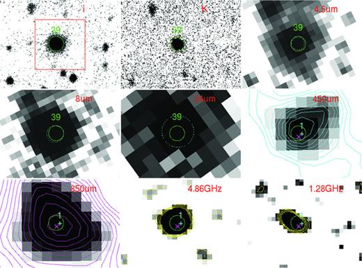
Finding charts for 850_1/450_1. From top left to bottom right: i (the size of the red box is 10 × 10 arcsec2), K, 4.5 μm (dashed cyan circle is the positions of the 4.5 μm sources with radius equal to the flux extraction radius), 8 μm (dashed cyan circles mark 8 μm sources and extraction radii), 24 μm (dashed cyan circles mark 24 μm sources and extraction radii), 450 μm (with cyan contours starting at 2σ and increasing in steps of 0.5), 850 μm (with magenta contours, starting at 2σ and increasing in steps of 0.5), 4.86 GHz (with yellow contours starting at 2σ and in intervals of 1), 1.29 GHz (with yellow contours, same as previous). All finding charts have the same FOV and the solid circles indicate the optical/NIR source position and extraction radius (green corresponds to 1.5 arcsec, red to smaller radii), only the sources mentioned in the text have been labelled. The labels have been omitted in the SCUBA and radio images for clarity, but we have labelled and marked instead with cyan ‘+’ our positions for the 450 μm sources and with magenta ‘x’ the positions of the 850 μm sources.

Finding charts for 850_2/450_2. Same layout as in Fig. 3.
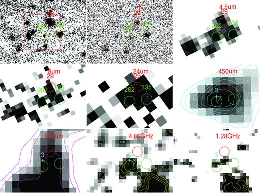
Finding charts for 450_3. Same layout as in Fig. 3.
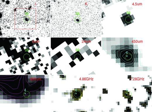
Finding charts for 450_4. Same layout as in Fig. 3.
It is worth noting the existence of a ‘blob’ of diffuse radio emission to the south-west (SW) of 450_3 (09:41:45.694 +38:54:07.57), clearly visible in both the VLA and Giant Metrewave Radio Telescope (GMRT) data with a diameter of about 3 arcsec. It appears to be connected to 450_3 by a bridge of ∼2σ emission in the former image. Its spectral index is α=−1.42 +0.18−0.14 which would advocate for it to be a lobe of radio emission. This area of diffuse emission is also clearly devoid of optical and Spitzer counterparts, which would be consistent with the lobe hypothesis. There is no evidence of a counterlobe to the north-east (NE) of 450_3. If it is a lobe, it could be associated instead with source 850_2/450_2, which is much brighter in radio, but no bridge of emission is seen between the latter source and the ‘blob’.
4.2 Association to submm sources, SEDs and SFR
The best-fitting (to RiZJK, 4.5 and 8 μm) photometric redshift templates are shown as red lines in Fig. 2, as well as the observed wide-band SEDs with a number of templates. We have plotted finding charts in i, K, Spitzer, SCUBA, VLA and GMRT for the five distinct sources from S10 (see Figs 3–7). All the redshift confidence intervals given in the rest of this section are 1σ.
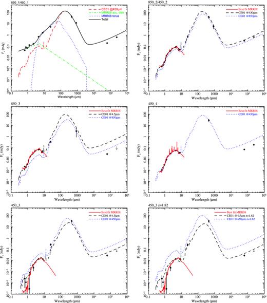
SED in Fν in the observer's frame for 850_1/450_1 (RX J0941, top left-hand panel), 850_2/450_2 (top right-hand panel), 850_3 (middle left-hand panel), 450_4 (middle right-hand panel) and 450_3 (with templates at the best photometric redshift – bottom left-hand panel – and fixed at z = 1.82– bottom right-hand panel). Observed points (RiZJK, 4.5, 8, 24, 450 and 850 μm, and 6 and 20 cm) are shown as black dots and upper limits as down-pointing arrows. The meaning of each line is summarized in each panel and explained fully in Section 4.2.
The templates from MRR08 do not include dust emission, so in order to model adequately the longer wavelengths we have used the starburst models of Chary & Elbaz (2001, hereafter CE01), which have been obtained from observations at several NIR–FIR wavelengths requiring the relative fluxes in different bands to be consistent with the observed IR luminosity functions. One feature of these models which is worth noting is that their shape is luminosity dependent and hence, given a redshift and the flux in one band, the SED is fully defined. The authors have provided idl routines to compute their templates at a given redshift and through a number of instrumental bandpasses. We have added the SCUBA 450 and 850 μm sensitivity curves to the set of available bandpasses. The absence of a good correlation between the B-band and IR luminosities implies that the optical/NIR part of their SEDs is uncertain. This is not a major problem here since we are only using the CE01 SEDs for the longer wavelengths. Instead of performing a formal χ2 fit to the data, we have computed the CE01 templates corresponding to each of the observed Spitzer and SCUBA fluxes at the redshift of each source.
In the case of 850_1/450_1, we expect to have a strong AGN component, especially in the rest-frame optical/NIR part of the spectrum. We have modelled it using templates from MRR08. We have approximated their RR1v2 AGN template with a broken power law (which is a good approximation to the continuum shape), redshifting it to z = 1.82 (the redshift of RX J0941). Within the Unified Model for AGN (Antonucci 1993), part of this direct emission is intercepted by a dusty torus, which ‘reprocess’ it and emits it at MIR and FIR wavelengths. To model this emission, we have used the dust torus template from MRR08.
We now discuss the counterparts to the submm sources and the SEDs individually.
850_1/450_1: the sharp radio contours prove that this source is indeed the central QSO (RX J0941). It is associated with source 39 (242/180 in S10). The full SED for this object is shown in Fig. 2 (top left-hand panel). The dashed red line represents the CE01 template normalized to the observed 450 μm flux at z = 1.82. It clearly reproduces well the observed emission at 450 μm and redwards, but it falls well short of the observed values bluewards of that wavelength. We have fitted the RiZJK fluxes with our broken power-law model for the ‘direct’ AGN emission from MRR08 (green dot-dashed line), which more or less follow the blue spectrum in the observed optical/NIR part of the SED, but again fails to account for the observed MIR emission. We have added the starburst emission to the direct AGN emission, subtracted it from the 8 μm point and rescaled the dust torus emission from MRR08 to this value (blue dotted line). The sum of these three components is shown as the black solid line in the figure. It clearly follows the overall shape of the SED, which cannot be reproduced by any two of the models alone. The submm emission is clearly dominated by the starburst, with the total AGN contribution being at least 2 orders of magnitude smaller, as originally stated in Page et al. (2001). There is very little room for an additional radio contribution from the AGN in this radio-quiet (RQ) QSO.
850_2/450_2: the radio data show a strong point-like source, coincident with our source 140 (191/155 in S10). Its photometric redshift is zp = 1.85 with a redshift interval spanning 1.83–2.16 with spectral type Sab. Our source 16 is about 2.2 arcsec away from 140, and could be contributing to its 24 μm flux. Its photometric redshift is 3.0 (2.9–3.0, Scd). Source 13 is brighter and coincides with elongations in the contours at 450 and 850 μm. Its photometric redshift is zp∼ 1.19 ± 0.03 (Scd), and hence is probably unrelated to the central QSO. In Fig. 2 (top right-hand panel), the dashed and dotted lines show the CE01 templates normalized to 450 and 850 μm, respectively. These lines straddle very closely all bluer and redder wavelengths.
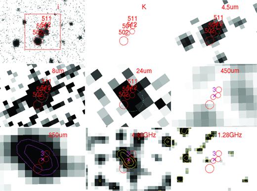
850_3: the NE–SW elongated 2σ and 2.5σ850 μm contours are aligned with the VLA 2σ contour. However, there is no sign of it in the GMRT image. This peak would favour our source 501 as the preferred counterpart (zp = 1.85, z in 1.83–2.20, Sab, 339/241 in S10), although this optical/NIR neighbourhood is rather crowded: sources 502, 511 and 512 are also close. The Spitzer emission appears point like favouring either 501 or 512. Unfortunately, the absence of J and K data for this area does not allow to put strong constraints on the photometric redshift range for 512 (zp∼ 0.7, SB). In Fig. 2 (middle left-hand panel), the CE01 template normalized to the 850 μm flux (blue dotted line) reproduces reasonably well all spectral points redwards of 8 μm, but falls well short at bluer wavelengths, although the spectral shape is similar. Normalizing the CE01 template to the 4.5 μm flux is a bit too high at 24 and 850 μm, and too high at radio wavelengths.
450_3: the 450 and 850 μm contours are complex (this source might also be detected in 850 μm, see Section 2) The >2σ VLA contour includes the 450 μm peak of 450_3, coinciding with our source 262 (206/160 in S10), and hence is our preferred counterpart. Object 262 comes originally from a 4.5 μm detection and only has upper limits in iZJ; hence, its redshift is poorly constrained, seeming to prefer zp∼ 2.8 (youngE, z > 2.6). Its absolute B magnitude would be too faint for both z = 1.82 and 2.8, suggesting an even higher redshift. This source seems to be connected by a 2σ bridge of radio emission to the radio ‘blob’ discussed in Section 4.1. Nearby sources with some evidence for Spitzer emission are 135 (205/159 in S10, zp = 1.85,1.8–2.2, Scd) and 29 (to the NW and along a NS elongation in the 850 μm contours, zp = 2.7, 2.6–2.9, SB). Object 135 coincides with the main east–west asymmetry of the 450 μm emission and could be related to the central QSO, although the absence of a radio detection does not support this idea. Since the redshift of 262 is poorly constrained, we show the CE01 SED normalized to the IRAC 4.5 μm and SCUBA points both at z = 2.78 (bottom left-hand panel) and at the redshift of the QSO z = 1.82 (bottom right-hand panel). The CE01 template normalized to the 450 μm point is well above the radio and the 4.5 and 8 μm points in both cases, while when it is normalized to the 4.5 μm point it matches better the IRAC and the radio points. This may mean that there might be some contribution to the SCUBA flux from our source 135, in agreement with the elongated contours at 450 μm. The 24 μm source position is intermediate between 262, 135 and 29, so the flux in that range also probably includes contribution from them, explaining why it lies above the CE01 template at z = 2.78.
450_4: it coincides with a well-defined point-like IRAC, VLA and GMRT source, very close to our source 98 (the unlabeled source to the W of the centre of the finding chart for 450_4 in S10). We have found zp = 1.85 (1.8–2.1, Sbc). Its SED is plotted in Fig. 2 (middle right-hand panel), showing that the CE01 models at that redshift neatly follow the shape of the Spitzer and SCUBA points (only the one normalized to the SCUBA point is shown, the models normalized to the Spitzer points are indistinguishable in this scale). The only clearly discrepant range is radio, which falls a factor of about 3 below the CE01 template.
In summary, the radio positions allow assigning unambiguous counterparts to all of the submm sources. Four out of five submm sources (850_1/450_1 – RX J0941, 850_2/450_2, 450_4 and 850_3) have counterparts with redshifts compatible with 1.82 within ∼1σ. The three latter ones have very similar spectral shapes, compatible with an existing relatively old stellar population with ongoing star formation. The last submm source (450_3) appears to be a radio emitting object at higher redshift, although there is a nearby counterpart within the ‘right’ redshift interval and very similar properties to the other counterparts to the submm sources (135). From the number counts in Coppin et al. (2006), we would expect to have about one submm source unrelated to the QSO in our field, so it is not surprising that 450_3 turns out to be a ‘background’ object, considering also its radio faintness.
4.3 Upper limits on AGN luminosities and estimating black hole masses
850_1/450_1 is the central QSO, and hence it obviously harbours a powerful AGN. In this Section, we will concentrate on the rest of our submm sources. The ‘blob’ of radio emission close to 450_3 might be interpreted as evidence for the presence of an AGN in this object. This possibility cannot be rejected using our current data due to its quality at the bluer wavelengths, where the AGN would be expected to dominate.
The optical-to-radio SEDs of the other three counterparts to the SCUBA sources have very limited room left for an additional AGN emission component. We will derive below limits to the luminosity of any putative AGN and the mass of the associated SMBH, under the assumption that the latter is growing through accretion, and radiation is emitted in the process. Our galaxies could harbour SMBH more massive than deduced below if they were dormant.
We have taken advantage of our XMM–Newton observation of this field (Page et al. 2011) to set limits on the intrinsic luminosity of any such AGN (see Section 2). Of course, the central QSO is actually detected (see Page et al. 2011). Three other SCUBA sources have upper limits on the pn camera (850_3 is in a gap between two chips in that camera), with similar values of <0.000 34 (<0.000 455) count s−1 in the 0.5–2 keV – soft – (2–10 keV – hard) band (using a simple power law with photon index Γ = 1.9 and local Galactic absorption; these values correspond to fluxes of about <6 × 10⁻¹⁶ and <4 × 10⁻¹⁵ erg cm−2 s−1, respectively). We have taken these count rates and estimated what would be the intrinsic luminosity of a z = 1.82 AGN to produce those count rates if viewed through different amounts of intrinsic absorption, parametrized as the Hydrogen column density NH. We have used NH = 0 and log(NH cm−2) = 21.5–25.5 in steps of 1 dex. We adopt a simply parametrized AGN spectral model following Gilli, Comastri & Hasinger (2007), i.e. an exponentially cut-off absorbed power law of photon index Γ = 1.9, a small scattered component, a reflection component and an Fe K emission line. We include a correction for Compton scattering of the continuum at the highest column densities. We have used the program xspec and an on-axis response matrix and ancillary file for pn to convert from count rates in those bands to luminosities in the rest frame 2–10 keV band LX,2−10 keV. The results are shown in Fig. 8.
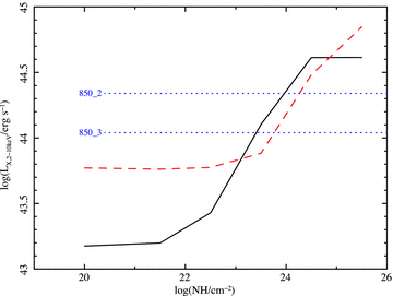
Upper limits to the 2–10 keV intrinsic luminosity of an AGN from the upper limits to the soft band (black solid line) and hard band (red dashed line) count rates from XMM–Newton observations versus the intrinsic column density. The value for NH = 0 has been plotted at log(NH/cm−2) = 20. The blue dotted lines mark the limits from the observed 24 μm fluxes for sources 850_2 and 850_3 (see text for an explanation).
Supernovae and binary stars associated with star formation produce X-rays, which would further reduce the allowance for any AGN emission. Ranalli, Comastri & Setti (2003) found a tight correlation between X-ray luminosity and FIR luminosity in local starburst galaxies which, using equation (1) above (Kennicutt 1998), can be expressed as SFR (M⊙ yr−1) = 2 × 10−40LX,2−10keV(erg s−1) (their equation 15). For the typical values of our galaxies of SFR ∼ 2000 M⊙ yr−1, this corresponds to LX,2−10 keV∼ 1043 erg s−1, comparable with the above upper limits for the soft band and moderate absorption.
In addition, we can set very conservative upper limits to the presence of an obscured AGN from the observed 24 μm flux. We have used as fiducial values those of sources 850_2 and 850_3 (∼700 and ∼350 μJy, respectively), because 450_4 is not detected in that band and 450_3 is probably a background source and its emission in that band is probably a blend of several sources. Assuming that the emission from dust heated by the AGN at 24 μm is isotropic and that the full observed fluxes at that wavelength have this origin, we can use an AGN SED (the Richards et al. 2006 RQ QSO template redshifted to z = 1.82) to find out what hard X-ray fluxes those 24 μm fluxes would correspond to. The corresponding values are log(LX,2−10 keV/erg s−1) = 44.3 and 44.0, respectively. Since the starburst SED template leaves very limited room for an additional AGN contribution (for instance, for 850_2 the difference between the 24 μm flux of CE01 template normalized to 450 μm and the actual observed flux at that wavelength is about 200 μJy, a factor of about 2 below our lowest fiducial value), this is an absolute ceiling to the maximum luminosity of a putative AGN in the innermost regions of our submm sources.
We conclude that AGN with intrinsic 2–10 keV luminosity ∼1043 erg s−1 could be present in our SCUBA sources if they are behind modest amounts of absorption [log(NH/cm−2) ≤ 22–23], while objects with almost QSO luminosities (∼1044 erg s−1) would have to be hiding behind much more substantial amounts of material [log(NH/cm−2) > 24]. More luminous AGN are not compatible with our current data. An X-ray luminosity of ∼1044 erg s−1 is compatible with the observed hard X-ray luminosities of SMGs at similar X-ray fluxes (Alexander et al. 2005)
4.4 Dust masses
For Fν, we have used the monochromatic fluxes at λ = 450 and 850 μm from Table 1. In order to estimate a range of dust masses for each object, we have used the eight possible combinations of (κ0 = 0.04 m2 kg−1, λ0 = 1.2 mm) (Beelen et al. 2006) and (κ0 = 2.64 m2 kg−1, λ0 = 125 μm) (Dunne, Eales & Edmunds 2003) with (T = 47 K, β = 1.6) (representative of unobscured quasars at high redshift; Beelen et al. 2006) and (T = 35 K, β = 1.5) (representative SMGs; see Kovács et al. 2006) and with the minimum and the maximum of the 1σ uncertainty interval in their photometric redshifts, taking the minimum and the maximum values of those combinations (which always corresponded to the minimum redshift, higher κ0, higher T and maximum redshift, higher κ0, lower T, respectively). We have made two exceptions: 850_1/450_1 (the QSO) for which we have fixed z = 1.82, and 450_3 for which we give both the intervals fixing z = 1.82 (main body of the table) and allowing the full photometric redshift uncertainty interval (footnote e of Table 1).
An additional source of uncertainty comes from the errors on the submm fluxes, which range from about 10 per cent to about 40 per cent (with one case reaching 70 per cent). These fractional errors are generally smaller than the uncertainty ranges derived above, and therefore we take the latter to represent a good estimate of the order of magnitude of the dust masses present in our sources.
For the sources detected at both submm wavelengths, we find that the dust mass estimates derived from 450 and 850 μm are compatible within the uncertainties. All sources have dust masses in the range 2 × 10⁸ – 3 × 10⁹ M⊙.
We can also estimate the gas mass present in the central regions of those galaxies from the dust masses, assuming a gas-to-dust ratio of 54, deduced by Kovács et al. (2006) for z = 1–3 SMG (with an uncertainty of about 20 per cent). This value is similar to the one obtained by Seaquist et al. (2004) for the central regions of nearby SCUBA galaxies. For our typical dust mass of ∼109 M⊙, this corresponds to a gas mass of ∼5 × 10¹⁰ M⊙.
4.5 Galaxy stellar masses
We have obtained MK at the best photometric redshift integrating the best-fitting template using hyperz. These estimates should be reasonably accurate for the sources with IRAC detections up to z∼ 2.6, since the best-fitting template would then be ‘anchored’ in a photometric point on a neighbouring rest-frame wavelength.
A further source of uncertainty is the assumed L/M. MRR08 use a different approach to estimate the stellar masses from the 3.6 μm luminosities of their best-fitting templates, with a L/M that depends on the galaxy class and on the cosmic time. We have also estimated the stellar masses of our three counterparts following this recipe. We obtain L/M = 0.05–0.06 and  for 450_4, 850_2 and 850_3, respectively. These stellar masses are between two and three times larger than those in Table 1, the discrepancies being larger than the total error budget calculated above.
In what follows, we will use for our sources a fiducial value log(M*/M⊙) = 11.5 ± 0.2 which takes into account the different stellar mass values for the different sources and the redshift and photometric uncertainties discussed above. Using the MRR08 recipe would produce values higher by 0.3–0.5 dex.
These stellar masses are similar to those obtained for other samples of SMGs: e.g. Borys et al. (2005) find log(M*/M⊙) = 11.4 ± 0.4 in the Chandra Deep Field (CDF)-N/GOODS-N region, and Michałowski, Hjorth & Watson (2010) find log(M*/M⊙) = 11–12 with a median of 11.7, despite using very different SEDs and methods for deriving the stellar mass (in the second case). As pointed out by Borys et al. (2005), those stellar masses are about 10 times larger than those of typical UV-selected star-forming galaxies at similar redshifts (Shapley et al. 2005). They are compatible with Schechter stellar mass for the GOODS-MUSIC galaxies at z∼ 1.8 (log(M*/M⊙) ∼ 11.3 ± 0.15 Fontana et al. 2006). They also similar to the Schechter mass of 3.6–4.5 μm selected galaxies in the Hubble Deep Field (HDF-N), CDF-S and the Lockman Hole in the 1.6 < z≤ 2.0 redshift interval [log(M*/M⊙) = 11.40 ± 0.18; Pérez-González et al. 2008]. Their 0 < z < 0.2 galaxies have slightly smaller masses [log(M*/M⊙) = 11.16 ± 0.25], although compatible within 1σ.
Although the above masses are stellar masses for the whole galaxy, they are probably dominated by the spheroid (as discussed by Borys et al. 2005; Alexander et al. 2008), since high-angular resolution H-band imaging of SMGs suggests that the stellar structure of most SMGs is best described by a spheroid/elliptical galaxy light distribution (Swinbank et al. 2010).
5 EVOLUTIONARY STAGE OF THE COUNTERPARTS
In this section, we use our estimates of the SFR and the stellar and dust mass for the counterparts to the submm sources to investigate their current state, their plausible future development and their relation to any putative AGN.
An immediate conclusion is that our SMGs are very mature; they have stellar masses typical of MIR and submm-selected galaxies (∼3 × 10¹¹ M⊙), and their gas masses (∼5 × 10¹⁰ M⊙) are around an order of magnitude smaller than our estimates of the stellar mass, indicating that ≳90 per cent of the maximum possible stellar mass is already in place.
Interestingly, Onodera et al. (2010) find a galaxy at a very similar redshift (z = 1.82) with a very similar stellar mass, which has properties fully consistent with those expected for passively evolving progenitors of present-day giant ellipticals. When the vigorous star formation taking place in our SMGs is over, they might well look like that object.
A common indicator of the strength of the star formation in galaxies is the specific SFR (SSFR) defined as the ratio of the SFR to the stellar mass. It is generally found that high-mass galaxies tend to have lower SSFR at z≲ 2 (see e.g. Feulner et al. 2005; Pérez-González et al. 2008; Ilbert et al. 2010), which is interpreted as a sign that star formation does not significantly change their stellar mass over this redshift interval. Our SMGs have SSFR ∼ 3–10 Gyr−1. These values are about an order of magnitude higher than those of MIR-selected galaxies with similar redshifts (1.6 < z≤ 2) and stellar masses [log(M*/M⊙) > 11] in Pérez-González et al. (2008). Our SMGs are amongst the most actively star-forming objects of their time.
Ilbert et al. (2010) find that, for a fixed range in SSFR, the fraction of high-mass objects among their star-forming galaxies drops with redshift between z = 2 and 1, while that of lower mass objects is approximately constant down to z∼ 1. This implies that the low-mass star-forming galaxies are able to maintain a high SSFR, while the massive galaxies evolve rapidly into systems with a lower SSFR (since the mass cannot go down, this means necessarily lower SFR). This is the expected evolution of our SMGs as deduced above from an independent argument, and follows a clear downsizing pattern (e.g. Cowie et al. 1996; Pérez-González et al. 2008).
Assuming that our SMGs host a SMBH which is growing and emitting radiation, in Section 4.3 (equation 5) we deduced a very conservative upper limit to the mass of the SMBH in AGN in the centre of our galaxies of log(M•/M⊙) < 8.1. Hence, their BH mass-to-galaxy mass ratio is log(M•/M*) < −3.4. Applying the relation between those quantities found by Marconi & Hunt (2003) for local galaxies, we get log(M•/M*) =−2.6[for log(M*/M⊙) = 11.5], so at face value our sources seem to have BH masses at least about a factor of 6 below local galaxies of the same mass. Other studies have also found lower SMBH-to-galaxy mass values in z∼ 2 SMG (e.g. Borys et al. 2005; Alexander et al. 2008; Coppin et al. 2009), which are commonly interpreted as the BH growth lagging behind the galaxy growth, since galaxies appear to be essentially fully grown while AGN are ‘undersize’.
There are considerable uncertainties in such estimates (as discussed at some length by e.g. Borys et al. 2005; Alexander et al. 2008). We include 0.2 dex of uncertainty in the stellar masses of our SMGs and the upper limit to the SMBH mass ranges between about 7.4 and 8.4 (in logarithmic solar masses) for different Eddington ratios and bolometric corrections (see Sections 4.3 and 4.5). Taking the extreme values for both masses, we get upper limits to log(M•/M*) between −2.9 and −4.3, while the value for local galaxies is log(M•/M*)local=−2.6 ± 0.3 (using the rms intrinsic dispersion quoted in Marconi & Hunt 2003, using instead Häring & Rix 2004 we would get −2.5 ± 0.3).
Hence the upper limit to the ratio we derived above between the local and our SMBH-to-galaxy mass is log(M•/M*)local/log(M•/M*) > 6, with an attached ‘uncertainty interval’∼1–100. The AGN in the centres of our galaxies would have to be heavily obscured and just at the limit of detection for that ratio to be close to unity. The X-ray-obscured AGN in SMGs studied by Alexander et al. (2005) are indeed heavily obscured [80 per cent have log(NH/cm−2) > 23], but their average luminosity is LX,2−10 keV∼ 5 × 1043 erg s−1, leading to an additional factor of 2 on that ratio. Finally, another factor of 2 or 3 would be necessary if we used the MRR08 method for estimating the stellar masses.
In summary, our SMGs appear to be mature log(M*/M⊙) = 11.5 ± 0.2 and with limited scope of significant further increase in mass (remaining gas mass ∼5 × 10¹⁰ M⊙), while any putative AGN in their centres [log(M•/M⊙) ≲ 8.1] is probably smaller than those of local galaxies of similar mass (by a factor of more than 6) but with plenty of fuel to grow if it can tap the inferred gas mass: the mass that a SMBH at our derived upper limit needs to accrete to reach the local SMBH-to-gas mass ratio is only about 1.3 per cent of the total gas mass.
The QSO RX J0941 shows strong X-ray emission (luminosity of 3 × 1044 erg s−1), high SFR (a few thousand solar masses per year) and strong ionized winds (Page et al. 2011). Within the evolutionary scheme outlined in Section 1, all these clues would mean that the SMBH is starting to push away the material responsible for the star formation and the SMBH growth.
Finally, the properties of our SMGs are similar to those of similar objects in ‘blank field’ observations (e.g. Borys et al. 2005; Alexander et al. 2008, whose properties have been obtained with similar methods) despite being in a significant overdensity. Similar properties of ‘spike’ and ‘field’ SMGs at z∼ 1.99 have also been reported by e.g. Chapman et al. (2009). This indicates that the environment does not affect substantially the SMG properties. Galaxy interactions are commonly invoked to channel material to the internal regions of galaxies, triggering starbursts (Mihos & Hernquist 1994). We have mixed evidence: RX J0941 (850_1) and 450_4 appear isolated in the optical/NIR bands, while 850_2 and 850_3 are in crowded immediate environments. Unfortunately, we lack high angular resolution data around our sources to be able to constraint tightly their interaction history.
6 CONCLUSIONS
Using X-ray to radio data, we have studied the immediate environment of RX J0941, a z = 1.82 QSO with strong ionized winds visible in the UV and in X-rays (Page et al. 2011), which shows both strong submm emission and an overdensity of SMGs around it (Stevens et al. 2004;S10). Such high density regions are expected to form a galaxy cluster at z = 0 (Kauffmann 1996).
The 6 and 20 cm radio data confirm the presence of all the submm sources and help to pinpoint their observed-frame optical-to-MIR counterparts. We have obtained photometric estimates of their redshifts using hyperz to fit SWIRE galaxy templates (MRR08) to RiZJK and Spitzer-IRAC data.
We found that four of the five unique submm sources are indeed associated with the QSO. The fifth source appears to be a background source, perhaps with an associated lobe of radio emission. The photometric redshifts appear to be robust against using different sets of templates (Bruzual & Charlot 2003; MRR08).
Under the assumption that a growing SMBH is hosted by our SMGs, we have used X-ray upper limits and the observed 24 μm fluxes to estimate a very conservative upper limit to the X-ray luminosity (<1044 erg s−1) of such putative AGN [and hence a SMBH mass of log(M•/M⊙) < 8.1], even if Compton thick material is absorbing the direct AGN emission.
We have used the rest-frame optical-to-radio starburst templates of CE01 to estimate the SFRs of the host galaxy of the QSO and the SMGs, obtaining individual rates of 1000 M⊙ yr−1 or above (see Table 1). We have also estimated dust (∼109 M⊙) and gas (∼5 × 10¹⁰ M⊙) masses, assuming parameters typical of the centres of SMGs.
We have also estimated their stellar masses from their rest-frame K-band luminosities, finding log(M*/M⊙) ∼ 11.5 ± 0.2, in line with other mass estimates for SMGs (e.g. Borys et al. 2005), but about 10 times larger than typical UV-selected star-forming galaxies at similar redshifts.
An immediate conclusion (as also found for other samples of SMGs) is that they are mature galaxies, with large stellar masses and an inferred reservoir of gas that would only allow a further 10 per cent increase in mass at most.
At the same time, their SMBH masses are a least factor of ∼6 below that expected for their galaxy mass and the local SMBH-to-galaxy mass ratio (Marconi & Hunt 2003). This has also been found previously for other samples of SMGs and is commonly interpreted as the growth of the SMBH lagging behind the galaxy growth, since the latter is already fully matured while the AGN still requires substantial growth (Borys et al. 2005; Alexander et al. 2008; Coppin et al. 2009). Accretion of a few percent of the inferred gas mass on to the SMBH would be sufficient to reach the local mass ratio.
Further observations are required to understand better the issues discussed here. Deeper X-ray data would allow to place tighter limits on, or to actually detect, AGN emission from the SMGs. Forthcoming Herschel SPIRE and PACS data will ‘fill in’ the gaps in the FIR–submm SED, getting better estimates of the SFR and dust masses. High angular resolution millimetre observations would give more accurate estimates of the gas mass. Photometric redshifts and SED studies for the other overdensities of SMGs in our sample (S10) will assess their relationship with the central QSOs and their evolutionary status, helping to understand the role of these high density peaks in the formation and evolution of galaxies.
The authors thank the anonymous referee for helpful suggestions to clarify the paper. FJC thanks M. Rowan-Robinson for his help with the SWIRE templates, R. Pelló for her help with hyperz and N. Benítez for his help with bpz. FJC, JE and SF acknowledge financial support from the Spanish Ministerio de Educación y Ciencia (later Ministerio de Ciencia e Innovación) under projects ESP2006-13608-C02-01 and AYA2009-08059. FJC, JAS and MJP acknowledge further support from the Royal Society. Based on observations made at the William Herschel Telescope and at the Isaac Newton Telescope which is operated on the island of La Palma by the Isaac Newton Group in the Spanish Observatorio del Roque de los Muchachos of the Instituto de Astrofísica de Canarias. Also based on observations obtained at the Gemini Observatory (under programme GN2004A-Q-52), which is operated by the Association of Universities for Research in Astronomy, Inc., under a cooperative agreement with the National Science Foundation (NSF) on behalf of the Gemini partnership: the National Science Foundation (United States); the Science and Technology Facilities Council (United Kingdom); the National Research Council (Canada); CONICYT (Chile); the Australian Research Council (Australia); Ministério da Ciência e Tecnologia (Brazil) and Ministerio de Ciencia, Tecnología e Innovación Productiva (Argentina). UKIRT is operated by the Joint Astronomy Centre, Hilo, Hawaii on behalf of the UK Science and Technology Facilities Council. Also based on observations made with the Spitzer Space Telescope, which is operated by the Jet Propulsion Laboratory, California Institute of Technology, under National Aeronautics and Space Administration (NASA) contract 1407. The James Clerk Maxwell Telescope (JCMT) is operated by The Joint Astronomy Centre on behalf of the Science and Technology Facilities Council of the United Kingdom, the Netherlands Organization for Scientific Research and the National Research Council of Canada. JCMT data were taken under project ID M03AU46. Also based on data collected at the XMM–Newton, an ESA science mission with instruments and contributions directly funded by ESA Member States and NASA. This research has made use of data obtained from the SuperCOSMOS Science Archive, prepared and hosted by the Wide Field Astronomy Unit, Institute for Astronomy, University of Edinburgh, which is funded by the UK Science and Technology Facilities Council. The NRAO is a facility of the National Science Foundation operated under cooperative agreement by Associated Universities. We thank the staff of the GMRT who have made these observations possible. GMRT is run by the National Centre for Radio Astrophysics of the Tata Institute of Fundamental Research. This publication makes use of data products from the 2MASS, which is a joint project of the University of Massachusetts and the Infrared Processing and Analysis Center/California Institute of Technology, funded by the NASA and the NSF. Funding for the SDSS and SDSS-II has been provided by the Alfred P. Sloan Foundation, the Participating Institutions, the NSF, the US Department of Energy, the NASA, the Japanese Monbukagakusho, the Max Planck Society and the Higher Education Funding Council for England. The SDSS is managed by the Astrophysical Research Consortium for the Participating Institutions. The Participating Institutions are the American Museum of Natural History, Astrophysical Institute Potsdam, University of Basel, University of Cambridge, Case Western Reserve University, University of Chicago, Drexel University, Fermilab, the Institute for Advanced Study, the Japan Participation Group, Johns Hopkins University, the Joint Institute for Nuclear Astrophysics, the Kavli Institute for Particle Astrophysics and Cosmology, the Korean Scientist Group, the Chinese Academy of Sciences (LAMOST), Los Alamos National Laboratory, the Max-Planck-Institute for Astronomy (MPIA), the Max-Planck-Institute for Astrophysics (MPA), New Mexico State University, Ohio State University, University of Pittsburgh, University of Portsmouth, Princeton University, the United States Naval Observatory and the University of Washington.
REFERENCES
Appendix
APPENDIX A: APERTURE MATCHING OF THE PHOTOMETRIC POINTS
Since each of our five optical–NIR images has a different seeing, we need to smooth all of them so that the effective seeing is the same as the one with the worst value (Z in our case). We have done this using gaus in iraf.
We have chosen a default aperture of 1.5 arcsec radius, which corresponds to ∼98 per cent enclosed flux for a 2D Gaussian with FWHM equal to the effective seeing (or 96 per cent for the empirical aperture correction explained below). There are 75 sources closer than 3 arcsec to another source so that the default aperture would assign counts from the same pixels to at least two sources. To avoid this, for each source we have chosen an aperture which is the minimum of 1.5 arcsec and half the distance to the closest source (in steps of 0.1 arcsec). The minimum aperture found using this method is 0.6 arcsec.
The flux F of each source is determined (using phot within iraf) from the number of counts within the chosen aperture (after background subtraction) and the magnitude from the usual −2.5 log F. The default phot procedure to obtain the uncertainty in the magnitude involves determining the mean value (msky) and the standard deviation (stdev) of the pixel values over the background area. This value can also be used to estimate the 1σ limit for the flux of each source as  (assuming Poisson statistics), where area is the area for the extraction of the source counts.
Following this recipe produces both too low values for the magnitude errors and unrealistically low flux limits. We believe that this is because the reduction processes outlined in Section 2 imply co-adding many individual images with rescalings to match median or average pixel values over essentially arbitrary areas. Furthermore, since we have smoothed the images to have the same ‘effective’ seeing, we have introduced correlations between the values of neighbouring pixels and essentially averaging away the dispersion in the sky values. This is bound to alter the statistical characteristics of the counts in each final pixel, with respect to the naïve Poisson assumption underlying most photometry packages (like phot).
We have followed an alternative approach. For each image, we have excluded an area of radius 2.5 arcsec around each source and, for each aperture radius, we have placed at random a large number (700) of circles of that size on the image, and we have measured the standard deviation (skydev) of the values of the fluxes within the simulated apertures, scaled to the total circle area. We have only kept simulated apertures in which more than 99 per cent of their area was outside the excluded zones. The number of simulated apertures has been chosen not to oversample the un-excluded area. We have checked that reducing the fraction of good pixels to 90 per cent, increasing the exclusion radius to 3 arcsec or increasing the number of simulated apertures to 2000 does not change the obtained values. The error on the fluxes can then be estimated as  and the 1σ upper limits as m0− 2.5 log10(skydev), where epadu is the e− ADU−1 of the detector and m0 are the zero-point magnitudes given in Table 2. The 1σ limits obtained in this way are shown in Table A1 in terms of magnitudes. In order to get, for example, 5σ limits, 2.5 log10(5) ∼ 1.75 needs to be subtracted from those values.
1σ upper limits for each image and aperture (see Appendix A).
| Aperture (arcsec) | R | i | Z | J | K |
| 0.6 | 27.06 | 27.41 | 26.26 | 24.67 | 23.44 |
| 0.7 | 26.76 | 27.05 | 26.02 | 24.43 | 23.08 |
| 0.8 | 26.55 | 26.86 | 25.85 | 24.13 | 22.86 |
| 0.9 | 26.28 | 26.73 | 25.64 | 23.93 | 22.65 |
| 1.0 | 26.15 | 26.49 | 25.49 | 23.74 | 22.51 |
| 1.1 | 25.95 | 26.38 | 25.40 | 23.60 | 22.34 |
| 1.2 | 25.80 | 26.25 | 25.21 | 23.47 | 22.21 |
| 1.3 | 25.68 | 26.14 | 25.10 | 23.32 | 22.08 |
| 1.4 | 25.51 | 25.99 | 25.01 | 23.17 | 21.99 |
| 1.5 | 25.40 | 25.89 | 24.89 | 23.06 | 21.91 |
This problem is also present in the Spitzer images, so we have obtained skydev for them in the same way as for the optical–NIR images, using the source extraction radii given in Section 2.1. Since those images were in units of MJy sr−1, the errors on the fluxes obtained by SExtractor (assuming Poisson statistics) were underestimated, and very similar for all sources (since they were dominated by the variance of the pixel values in the background). We have used the FLUXCONV and GAIN keywords in the headers of the 4.5 and 8 μm images4 and the exposure times to estimate the original number of counts in the image and the corresponding errors. The total uncertainty in the image fluxes was obtained by adding to these errors in quadrature the total uncertainty in the determination of the values of those keywords (about 5 per cent, see footnote) and the uncertainty in the sky values (skydev). These fluxes and errors are the ones used for the empirical flux calibration described in 2.1. After applying this calibration, the 1σ sky standard deviations in the 4.5, 8 and 24 μm bands are 0.5, 2.1 and 52 μJy, respectively.
In order to obtain a good estimate of the stellar mass, it is essential to have a good measurement of the rest-frame K-band absolute magnitude, which would fall between the IRAC bands at the redshift of RX J0941. Hence, it is essential to include those bands in the photometric redshift fits for the 101 sources detected in either of those two MIR bands. But, since the Spitzer fluxes are corrected to ‘infinite’ aperture, good estimates of this correction for the optical–NIR fluxes are needed as well, so that all the photometric points fed to the fit match.
We have done this empirically, extracting for each source a radial profile in the smoothed i-band image between 0.2 arcsec and half the distance to the nearest source (see above) and fitting to it both a single and a double Gaussian profile, allowing thus for both ‘nuclear’ and ‘galaxy’ components. We have chosen for each source the best fit between those two using an F-test. The average value of the σ of a single Gaussian profile (for the sources for which this was the best fit) is 0.59 arcsec, slightly larger than the one used for matching the angular resolution of all optical–NIR images (0.54 arcsec), but essentially compatible with it. A correction factor was then calculated from the best-fitting profile for each source.
The fluxes/magnitudes of the 101 sources with 4.5 or 8 μm detections have been corrected with this factor before the photometric redshift fitting, so the derived physical magnitudes are already for ‘infinite’ aperture. For the remaining 138 sources, this factor has been applied to these derived magnitudes after the photometric redshift fit.
