Magnetothermal and magnetorotational instabilities in hot accretion flows

Abstract

1 INTRODUCTION

Hot, diffuse accretion flows are likely to be present in low-luminosity active galactic nuclei (AGNs) and the quiescent and hard states of black hole X-ray binaries (Narayan 2005; Yuan 2007; Narayan & McClintock 2008). When the mass accretion rate is very low, the electron mean-free path will be very large, so the accreting plasma is nearly collisionless. For example, from Chandra observations of the accretion flow at the Galactic Centre, Sgr A*, the electron mean-free path is estimated to be 0.02–1.3 times the Bondi radius (∼10⁵–10⁶ Schwarzschild radii). In such cases, thermal conduction can have a significant influence on the dynamics (Quataert 2004; Johnson & Quataert 2007), resulting in the transport of thermal energy from the inner (hotter) to the outer (cooler) regions. If the energy flux carried by thermal conduction is substantial, the temperature of the gas in the outer regions can be increased above the virial temperature. Thus, gas in the outer regions is able to escape from the gravitational potential of the central black hole and form outflows, significantly decreasing the mass accretion rate (Tanaka & Menou 2006; Johnson & Quataert 2007).

Time-dependent hydrodynamical simulations of hot accretion flows show that they are convectively unstable, no matter whether the flow is radiatively inefficient (Igumenshchev & Abramowicz 1999, 2000; Stone, Pringle & Begelman 1999) or efficient (Yuan & Bu 2010). This is consistent with the prediction of one-dimensional analytical models of advection-dominated accretion flows (ADAFs; Narayan & Yi 1994, 1995). Convective instability occurs because the entropy of the flow increases in the direction of gravity. However, in a magnetized weakly collisional accretion flow, in which the electron mean-free path is much greater than the Larmor radius, thermal conduction is anisotropic and primarily along the magnetic field lines. In this case, Balbus (2000, 2001) found that the stability criterion for convection is fundamentally altered: convection occurs when the temperature – not the entropy – increases in the direction of gravity. Convective instabilities in this regime are referred to as the magnetothermal instability (MTI).

In a weakly magnetized, non-rotating atmosphere, local simulations have demonstrated that the MTI can amplify the magnetic field and lead to a substantial convective heat flux (Parrish & Stone 2005, 2007). Sharma, Quataert & Stone (2008, hereafter SQS08) investigated the effects of the MTI on accretion flows in two dimensions using global simulations in spherical polar coordinates. Their simulations focused on the region around the Bondi radius, where the MTI growth time is shorter than the gas infall time. They found that the MTI can amplify the magnetic field and align field lines with the direction of the temperature gradient (radially), consistent with the results obtained by previous local simulations. The effects of the MTI on the intracluster medium (ICM) have also been investigated (Parrish, Stone & Lemaster 2008). In that study also, the MTI drives the magnetic field lines to be radial, leading to a conductive flux, which is an appreciable fraction of the classical Spitzer value. Such a high rate of thermal conduction makes the slope of the temperature profile flatter.

The studies of the MTI described above all focus on a non-rotating accretion flow. It is well known that in a weakly magnetized, differentially rotating hot accretion flow, the magnetorotational instability (MRI; Balbus & Hawley 1991, 1998) will be present. Also, magnetohydrodynamics (MHD) turbulence driven by the MRI is thought to be the most promising mechanism of angular momentum transport. In principle, the MTI and MRI should coexist in such flows. Therefore, an interesting question for investigation is whether the MTI and MRI interact with one another; that is, does one instability enhance or suppress the other, or do the two instabilities operate entirely independently? For example, it is interesting to ask whether convective motions driven by the MTI can transport angular momentum, and similarly whether turbulent motions driven by the MRI can transport heat.

Motivated by the question above, we present the results of a two-dimensional MHD simulation of hot accretion flows with anisotropic thermal conduction and rotation. We investigate flows that are slowly rotating (not rotationally supported) at the Bondi radius, where the growth times of both the MTI and MRI are shorter than the infall time. This paper is organized as follows. We introduce our numerical methods and initial conditions in Section 2. Most of our results are presented in Section 3, while Section 4 is devoted to a summary and discussion.

2 NUMERICAL SIMULATION

We adopt two-dimensional, spherical coordinates (r, θ) and assume axisymmetry ∂/∂ϕ≡ 0. We use the Zeus-2D code (Stone & Norman 1992a,b) to solve the MHD equations with anisotropic thermal conduction:

1

2

3

4

5

Here, ρ is the mass density, v is the velocity, p is the pressure, ψ=−GM/r is the gravitational potential (where G is the gravitational constant and M is the mass of the central black hole), B is the magnetic field, e=p/(γ− 1) is the internal energy (where γ is the adiabatic index), Q is the heat flux along magnetic field lines, χ is the thermal diffusivity, is the unit vector along magnetic field and T is the temperature of the gas.

For convenience, we adopt χ=κp/T and assume that κ=a_c(GMr)^1/2, which has the dimension of a diffusion coefficient (cm² s⁻¹). Anisotropic thermal conduction is implemented using the method based on limiters (Sharma & Hammett 2007) to guarantee that heat always flows from hot to cold regions.

We initialize our simulations as follows. The radial velocity, internal energy and density of the accretion flow are adopted from the hydrodynamic Bondi solution. For the other two components of the velocity (v_θ and v_ϕ), we set v_θ = 0 and v_ϕ=l₀/r where l₀ (= const.) – a parameter of our simulations – is the specific angular momentum of the accretion flow. The initial magnetic field is uniform and perpendicular to the equatorial plane (i.e. B=B_z, where z is the vertical cylindrical coordinate). We have run four models. The parameters used in these models are listed in Table 1. In models L1 and L2, we set l₀ to be 0.1 times the Keplerian angular momentum at the inner boundary. Thus, in models L1 and L2, the centrifugal barrier is inside our inner boundary, and a rotationally supported region is never formed in these two models. In models H1 and H2, however, we set l₀ to be 10 times the Keplerian angular momentum at the inner boundary. Thus, in models H1 and H2, the centrifugal barrier is outside our inner boundary, so that a rotationally supported disc can form, which is subject to the MRI. We set β (the ratio of gas pressure to magnetic pressure) to be β = 10¹² at the outer boundary in our initial conditions. We assume that the adiabatic index γ = 1.5. We use the Bondi radius, r_B=GM/c²_∞ (c_∞ is the sound speed at infinity, and we set c²_∞ = 10⁻⁶c² where c is the speed of light) to normalize all of the length-scales in our paper. Times reported in this paper are all in units of the inverse rotation frequency at the outer radius of the domain, Ω⁻¹_out = (r³_out/GM)^1/2.

All of our calculations span a domain bounded by an inner boundary at r_in = 0.05r_B and an outer boundary at 20r_B. As in SQS08, we adopt a numerical resolution of 60 × 44. The radial grid is logarithmically spaced. A uniform polar grid extends from θ = 0 to π. At the poles, we use axisymmetric boundary conditions. In the radial direction, we use inflow/outflow boundary conditions at both the inner and outer boundaries. For the temperature at the inner and outer boundaries, we use outflow boundary conditions.

3 RESULTS

3.1 Magnetic field amplification

A weakly magnetized, conductive, differentially rotating accretion flow is subject to MTI and MRI when the following condition is satisfied:

6

Here, Ω is the angular velocity of the accretion flow. Provided that the magnetic field is weak, the condition for the existence of MTI alone is

7

This condition is always satisfied in the initial conditions of our calculations. Thus, as long as the MTI growth time is smaller than the gas infall time, the MTI will grow. The condition for the existence of the MRI is

8

This condition is again always satisfied in the initial conditions of our calculations. Defining

9

10

the MTI and MRI growth time-scales are then t_MTI=γ⁻¹_MTI and t_MRI=γ⁻¹_MRI, respectively. The wavelengths of the maximum growth rates for MTI and MRI are

11

and

12

respectively. Here, is the Alfvén speed.

We investigate the interplay between the MTI and MRI by examining the magnetic field amplification by the two instabilities. Note that, in addition to the MTI and MRI, the magnetic field can also be amplified by the geometric convergence of the accretion flow in spherical geometry and flux freezing. First, we investigate the magnetic field amplification by flux freezing by carrying out model L1. We note that in models L1 and L2, the centrifugal barrier is inside our inner boundary, and thus the time-scale for the MRI to grow is much longer than the gas infall time-scale. Furthermore, in model L1, we set the coefficient of the thermal diffusivity a_c = 0 (i.e. there is no MTI in model L1). Therefore, the magnetic field amplification in model L1 can only be a result of flux freezing. The results show that the effect of flux freezing on magnetic field amplification is very small, allowing us to ignore this effect in the analysis of models L2, H1 and H2.

In model L2, we set the coefficient of the thermal diffusivity a_c = 0.2 so that it is unstable to the MTI. In this model, the magnetic field is amplified only by the MTI. In models H1 and H2, the centrifugal barrier is outside our inner boundary. The time-scale for the growth of the MRI is much shorter than the gas infall time, so the MRI will affect the flow in both models. In model H1, we set the coefficient of the thermal diffusivity a_c = 0, so that the MTI is suppressed and the magnetic field is amplified only by the MRI. In model H2, we set the coefficient of the thermal diffusivity a_c = 0.2, so that both MTI and MRI coexist, and the magnetic field is amplified by the non-linear evolution of both. The properties of the four models are summarized in Table 1. The models demonstrate the interplay between the MTI and MRI. We have also tried various other values of a_c; we have found that changing a_c by a factor of a few does not affect our results, consistent with the conclusion in SQS08.

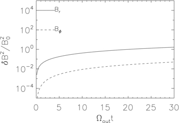
Figs 1–4 show the change of magnetic energy as a function of time in these four models. The energy is averaged from r=r_out/40 to r_out. The solid, dotted and dashed lines correspond to the energy in the r, θ and ϕ components of the magnetic field, respectively.

Figure 1

Evolution of the volume-averaged magnetic energy in both the r and ϕ components of the magnetic field normalized to the initial magnetic energy in a shell from r_out/40 to r_out in model L1. In this model, the magnetic field is amplified only by flux freezing. As v_θ∼ 0, there is almost no amplification of the θ component of the field, so it is not shown. The growth of each component is defined as δB²_r,θ,ϕ = (〈B²_r,θ,ϕ〉_V−B²_r,θ,ϕ,0), where 〈〉_V denotes volume average and B₀ is the initial field strength.

Open in new tabDownload slide

Figure 2

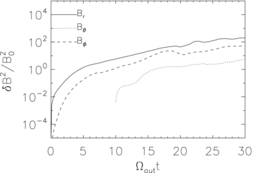
Change of volume-averaged magnetic energy in the r, θ and ϕ components of the magnetic field normalized to the initial magnetic energy in a shell from r_out/40 to r_out as a function of time in model L2. In this model, the magnetic field is amplified by the MTI. The growth of each component of the magnetic field is defined as δB²_r,θ,ϕ = (〈B²_r,θ,ϕ〉_V−B²_r,θ,ϕ,0), where 〈〉_V denotes volume average and B₀ is the initial field strength.

Open in new tabDownload slide

Figure 3

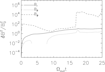
Change of volume-averaged magnetic energy in the r, θ and ϕ components of the magnetic field normalized to the initial magnetic energy in a shell from r_out/40 to r_out as a function of time in model H1. In this model, the magnetic field is amplified by the MRI. The growth of each component of the magnetic field is defined as δB²_r,θ,ϕ = (〈B²_r,θ,ϕ〉_V−B²_r,θ,ϕ,0), where 〈〉_V denotes volume average and B₀ is the initial field strength.

Open in new tabDownload slide

Figure 4

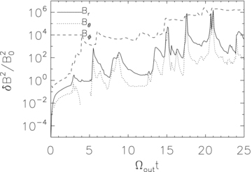
Change of volume-averaged magnetic energy in the r, θ and ϕ components of the magnetic field normalized to the initial magnetic energy in a shell from r_out/40 to r_out as a function of time in model H2. In this model, the magnetic field is amplified by both the MTI and MRI. The growth of each component of the magnetic field is defined as δB²_r,θ,ϕ = (〈B²_r,θ,ϕ〉_V−B²_r,θ,ϕ,0), where 〈〉_V denotes volume average and B₀ is the initial field strength.

Open in new tabDownload slide

Fig. 1 shows the magnetic energy evolution in model L1. The field is smoothly amplified by flux freezing. At the end of the simulation, the field is only amplified by a factor of 2. Because v_θ∼ 0, there is almost no amplification of the θ component of the field. From this model, we can see that the effect of flux freezing on magnetic field amplification is very small.

We now investigate the magnetic field amplification by the MTI (model L2). The only difference between models L1 and L2 is that in the latter we include thermal conduction so that the MTI is present. Fig. 2 shows the evolution of the magnetic energy in model L2. It shows significantly more amplification of the magnetic field in comparison to model L1. This amplification is mainly a result of motions driven by the MTI. Initially, the field is rapidly amplified by the MTI. After time t = 6, the magnetic field ceases to grow exponentially, and the growth rate becomes small, for the following reason. The growth rate of the fastest growing mode of the MTI is given by γ≃ |[1/ρ][dp/dr][d ln T/dr]|^1/2b_θ where b_θ=B_θ/B. The growth rate decreases with time because of the decrease of b_θ with time. In this model, we use parameters F_r,t, F_θ,t and F_ϕ,t to represent the amplification factors of the r, θ and ϕ components of the magnetic field, respectively. We find

13

14

15

Here, B_r,f, B_θ,f and B_ϕ,f correspond to the r, θ and ϕ components of the magnetic field at the end of the simulation, respectively. The radial component of the magnetic field is amplified by the MTI significantly. The MTI saturates by aligning field lines with the temperature gradient (radial direction), which is consistent with the results of previous work (Parrish & Stone 2005, 2007; SQS08). SQS08 found that the magnetic field amplification by MTI is quasi-linear. If the magnetic field is weak initially, the MTI can amplify the field by a factor of ∼10–30, independent of the initial field strength. Our calculation confirms their result.

We investigate field amplification by the MRI in model H1. In this model, we turn off thermal conduction so the MTI does not exist, and the magnetic field amplification must be a result of motions driven by the MRI. Fig. 3 shows the time evolution of the magnetic energy. Initially (t < 16.5), the field is very weak. At our resolution, the fastest growing mode of the MRI is not resolved, so the field amplification occurs primarily by flux freezing. The initial (t < 1) rapid amplification of the azimuthal component of the magnetic field is a result of shear. At t = 16.5, the magnetic field strength is amplified by flux freezing to a high enough value that the MRI is resolved, and the field undergoes substantial and rapid amplification by the MRI. To illustrate this point, we define a parameter Re=λ_MRI/Δx, where Δx is the grid size, which measures how well the MRI is resolved on our numerical grid. Fig. 5 shows the contours of Re at t = 16.5. From this figure, it is clear that the unstable wavelengths of the MRI are well resolved at that time. The MRI amplifies the field rapidly, and shortly after t = 16.5 the MRI saturates and the field begins to grow algebraically. Saturation of the MRI can be understood as follows. The condition for MRI to operate is k²v²_a+ dΩ²/d lnr < 0. After t = 18, we find k²v²_a+ d Ω²/d ln r∼ 0 in the region where the MRI growth wavelength can be resolved, so the growth rate of the MRI decreases significantly. Using parameters F_r,r, F_θ,r and F_ϕ,r to represent the magnetic field amplification factor of the r, θ and ϕ components of the magnetic field, respectively, we find

16

17

18

Here, B_r,f, B_θ,f and B_ϕ,f correspond to the r, θ and ϕ components of the magnetic field at the end of the simulation, respectively. The toroidal component is most significantly amplified as expected.

Figure 5

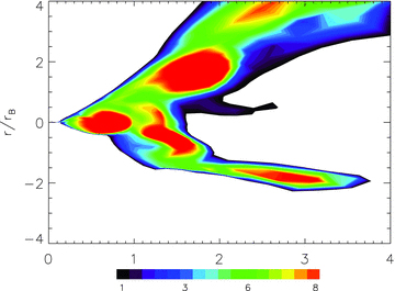
Contour of Re=λ_MRI/Δx at time t = 16.5, where Δx is the grid size. It is clear that the wavelength of the fastest growing mode of the MRI is well resolved at time t = 16.5.

Open in new tabDownload slide

In model H2, we turn on thermal conduction so both the MTI and MRI coexist. Fig. 4 shows the time evolution of the magnetic energy. Initially (t < 3), there is only the MTI. This is because, initially, the field is too weak for unstable wavelengths of the MRI to be resolved. At t = 3, the magnetic field has been amplified by the MTI enough that unstable modes of the MRI are resolved, and the MRI begins to drive motions. After t = 3, the field begins to be amplified exponentially by both the MTI and MRI, until at t∼ 20 both instabilities saturate and the growth of the field becomes algebraic. Using parameters F_r, F_θ and F_ϕ to represent the amplification factor of the r, θ and ϕ components of the magnetic energy, respectively, we find

19

20

21

Here, B_r,f, B_θ,f and B_ϕ,f correspond to the r, θ and ϕ components of the magnetic field at the end of the simulation, respectively.

Comparing models L2, H1 and H2, we find

22

23

24

Let us first consider the amplification of the radial component of the magnetic field. If the MTI alone amplifies the radial component of the magnetic energy by a factor of F_r,t (model L2), and the MRI alone by a factor of F_r,r (model H1), then when the MTI and MRI coexist the radial component of the magnetic field can by amplified by a factor of F_r,tF_r,r (model H2). The amplification factors for the other two components of the magnetic energy behave similarly. We therefore conclude that in the non-linear regime the MTI and MRI amplify the field independently. This is most likely because the MTI is a buoyancy instability driven by radial gradients in the temperature, while the MRI is a dynamical instability driven by the radial gradient of the orbital frequency. Provided that the magnetic field is weak and the plasma is dilute, thermal conduction from hotter to cooler regions will make the plasma buoyantly unstable, regardless of whether the flow also contains turbulent eddies driven by the MRI. However, provided that the magnetic field is weak and differential rotation exists, the MRI can operate regardless of the presence of convective eddies driven by the MTI.

3.2 Role of MTI in angular momentum transfer

The MRI is now believed to be the most promising mechanism of angular momentum transport in fully ionized accretion flows. It is interesting to investigate whether the MTI can contribute to angular momentum transfer in hot, diffuse accretion flows.

First, we compare the angular momentum profiles in models L1 and L2 at the end of both calculations. The flow in model L1 is laminar, while there is (only) MTI in model L2. The angular momentum profiles at the end of the simulations are shown in Fig. 6. It is clear that the angular momentum distribution of model L1 is almost the same as the initial distribution. This is because the flow in model L1 is laminar, and the magnetic field is very weak. Therefore, both the Reynolds and magnetic stresses are very small and there is almost no angular momentum transfer. It is also clear that in model L2, angular momentum is transferred from the inner to the outer regions. In order to investigate the mechanism for the angular momentum transport in this case, we plot the Maxwell and Reynolds stresses in Fig. 7. The dotted and solid lines correspond to the Maxwell stress (−B_rB_ϕ/4π) in models L1 and L2, respectively. Because of magnetic field amplification by the MTI, the Maxwell stress in model L2 is much larger than that in model L1. The triangles and squares denote the Reynolds stress in models L1 and L2, respectively. Because of the presence of motions driven by the MTI in model L2, the Reynolds stress is three orders of magnitude higher than in model L1. Because the magnetic field is still very weak in model L2, the Maxwell stress is much smaller than the Reynolds stress. We conclude that the angular momentum transport in model L2 is dominated by the Reynolds stress. We note that although the MTI induced Reynolds stress does transfer angular momentum, the effect is quite low, so that there is only a small change of the angular momentum profile compared to the initial conditions.

Figure 6

Radial profiles of specific angular momentum for models L1 (dotted line) and L2 (solid line). The dashed line shows the initial angular momentum distribution.

Open in new tabDownload slide

Figure 7

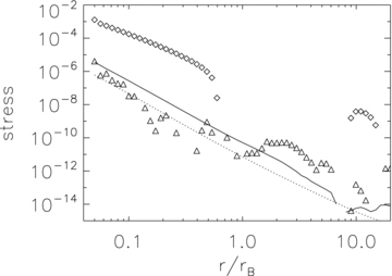
Radial profiles of stress. The dotted and solid lines correspond to the Maxwell stress in models L1 and L2, respectively. The triangles and squares are Reynolds stress in models L1 and L2, respectively.

Open in new tabDownload slide

Next, in Fig. 8, we compare the angular momentum distribution in models H1 and H2 at late times. Both profiles are similar. Recall that both models are unstable to the MRI, while only H2 is unstable to the MTI. The similarity in the angular momentum profiles indicates that the role of the MTI in angular momentum transport is less important compared to the MRI.

Figure 8

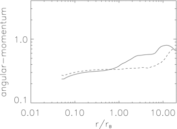
Radial profiles of specific angular momentum for models H1 (solid line) and H2 (dashed line).

Open in new tabDownload slide

3.3 Effects of MTI on the structure of the accretion flow

Fig. 9 shows the time-averaged density (upper-left panel), temperature (upper-right) and mass accretion rate (lower panel) for models H1 and H2. In the upper panels, the solid and dashed lines correspond to models H1 and H2, respectively. In the lower panel, the solid, dotted and dashed lines correspond to the net accretion rate, inflow rate and outflow rate, respectively. The black and red lines correspond to models H1 and H2, respectively. As shown in the upper-right panel, the radial profile of temperature in model H2 (with MTI) is flatter than that in model H1. This is likely because thermal conduction transports energy from the inner to the outer regions of the flow. From the lower panel, we can see that the inflow rate decreases because of the effects of thermal conduction. This is consistent with Johnson & Quataert (2007). The decrease is caused by the increased heating of the outer regions by thermal conduction.

Figure 9

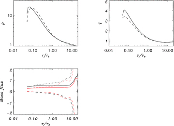
Radial profiles of time-averaged variables in models H1 and H2: density (upper-left panel) and temperature (upper-right panel). The lower panel shows the mass accretion rate. In the upper panels, solid and dashed lines correspond to models H1 and H2, respectively. In the lower panel, the solid, dotted and dashed lines correspond to the net accretion rate, inflow rate and outflow rate, respectively. The black and red lines correspond to models H1 and H2, respectively.

Open in new tabDownload slide

4 DISCUSSION AND SUMMARY

In extremely low accretion rate systems, the plasma is very dilute, and the collisional mean-free path of electrons is much greater than their Larmor radius. Thus, thermal conduction is anisotropic and along magnetic field lines. Anisotropic thermal conduction can fundamentally alter the Schwarzschild convective instability criterion. Convection sets in when temperature (as opposed to entropy) increases in the direction of gravity. Convective instability in this regime is referred to as the MTI. The MTI can amplify the magnetic field and align field lines with the temperature gradient (i.e. the radial direction). If the flow has angular momentum, the MRI may also exist. We have investigated the possible interaction between the MTI and MRI by performing two-dimensional MHD simulations of non-radiative rotating accretion flows with anisotropic thermal conduction.

We have presented the results from four models, with the focus on the amplification of magnetic energy by the combination of MTI and MRI. As a control case, we computed a model (L1) in which neither the MTI nor the MRI was present, so that the magnetic field is amplified only by flux freezing and geometrical compression in the flow. We find that field amplification via flux freezing in this case is very small. Next, we investigated the effects of the MTI on magnetic field amplification in model L2. We find that the MTI can amplify magnetic field significantly, which is consistent with the result obtained in previous work. Finally, we considered the evolution of rotating flows that are unstable to the MRI. In model H1 (no thermal conduction), only the MRI is present. In model H2, both the MTI and MRI coexist. By comparing the structure and evolution of these different models, we find that if the MTI alone can amplify the magnetic energy by a factor of F_t, and the MRI alone by a factor of F_r, then when the MTI and MRI are both present, the magnetic energy can be amplified by a factor of F_tF_r. Thus, we conclude that the MTI and MRI operate independently, and that there is little feedback on the amplification factor in the non-linear regime. Because the MTI and MRI are driven by different properties of the flow (temperature gradient for MTI and angular velocity gradient for MRI), the presence of one may not strongly affect the presence of the others. Thus, anisotropic thermal conduction can make the plasma buoyantly unstable, regardless of whether or not turbulent eddies driven by the MRI are present. Similarly, an unstable rotation profile can result in the MRI, regardless of whether or not there are convective eddies induced by the MTI.

In addition to the interplay between the MTI and MRI, we have also investigated the effects of MTI on angular momentum transport. We find that the MTI enhances angular momentum transport simply because it can amplify magnetic field (thus enhancing the Maxwell stress) and induce radial motions (thus enhancing the Reynolds stress). However, we note that the effects of the MTI on angular momentum transfer are small. Finally, we find that thermal conduction does make the slope of the temperature smaller because of the outward transport of energy, and the increase of the temperature in the outer regions decreases the mass accretion rate.

Lastly, we would like to mention that in a weakly collisional accretion flow, the ion mean-free path can be much greater than its Larmor radius, and thus the pressure tensor is anisotropic. In this case, the growth rate of the MRI can increase dramatically at small wavenumbers compared to the MRI in ideal MHD (Quataert, Dorland & Hammett 2002; Sharma, Hammett & Quataert 2003). In this regime, the viscous stress tensor is anisotropic, and Balbus (2004) has shown that when anisotropic viscosity is included, the flow is subject to the magnetoviscous instability (MVI); see also Islam & Balbus (2005). The MVI may also amplify the magnetic field significantly. An interesting project for the future is to investigate the effects of the MVI on hot accretion flows.

We thank P. Sharma for sending us his code. This work was supported in part by the Natural Science Foundation of China (grants 10773024, 10833002, 10821302 and 10825314), the National Basic Research Programme of China (973 Programme 2009CB824800) and the CAS/SAFEA International Partnership Programme for Creative Research Teams.

REFERENCES