


Abstract
We study the effects of anisotropic thermal conduction on low-collisionality, astrophysical plasmas using two- and three-dimensional magnetohydrodynamic simulations. Dilute, weakly magnetized plasmas are buoyantly unstable for either sign of the temperature gradient: the heat-flux-driven buoyancy instability (HBI) operates when the temperature increases with radius while the magnetothermal instability (MTI) operates in the opposite limit. In contrast to previous results, we show that the MTI can drive strong turbulence and operate as an efficient magnetic dynamo, akin to standard, adiabatic convection. Together, the turbulent and magnetic energies may contribute up to ∼10 per cent of the pressure support in the plasma. In addition, the MTI drives a large convective heat flux, up to ∼1.5 per cent ×ρc3s. These findings are robust even in the presence of an external source of strong turbulence. Our results for the non-linear saturation of the HBI are consistent with previous studies but we explain physically why the HBI saturates quiescently, while the MTI saturates by generating sustained turbulence. We also systematically study how an external source of turbulence affects the saturation of the HBI: such turbulence can disrupt the HBI only on scales where the shearing rate of the turbulence is faster than the growth rate of the HBI. The HBI reorients the magnetic field and suppresses the conductive heat flux through the plasma, and our results provide a simple mapping between the level of turbulence in a plasma and the effective isotropic thermal conductivity. We discuss the astrophysical implications of these findings, with a particular focus on the intracluster medium of galaxy clusters.
1 INTRODUCTION
The thermodynamics of a plasma can have dramatic and sometimes unexpected implications for its dynamical evolution. For example, thermal conduction can reduce the accretion rate in spherical accretion flows by as much as 2 to 3 orders of magnitude relative to the Bondi value (Johnson & Quataert 2007; Shcherbakov & Baganoff 2010). Additionally, Balbus (2000) and Quataert (2008) demonstrated that the convective dynamics of conducting plasmas differ significantly from those of an adiabatic fluid. This paper focuses on the non-linear evolution and saturation of this convection.
When anisotropic conduction is rapid compared to the dynamical response of a plasma, the temperature gradient, rather than the entropy gradient, determines the plasma’s convective stability. The convective instability in this limit is known as the heat-flux-driven buoyancy instability (HBI) when the temperature increases with height (g·∇T < 0), or as the magnetothermal instability (MTI) when the temperature decreases with height (g·∇T > 0). We summarize the linear physics of these instabilities in Section 2. Parrish & Stone (2005, 2007) and Parrish & Quataert (2008) studied the non-linear development of the MTI and HBI using numerical simulations. These instabilities couple the magnetic structure of the plasma to its thermal properties and potentially have important implications for galaxy clusters (Parrish, Stone & Lemaster 2008; Bogdanović et al. 2009; Parrish, Quataert & Sharma 2009; Sharma et al. 2009a; Bogdanović, Reynolds & Massey 2010; Parrish, Quataert & Sharma 2010; Ruszkowski & Oh 2010), hot accretion flows on to compact objects (Sharma, Quataert & Stone 2008) and the interiors and surface layers of white dwarfs and neutron stars (Chang & Quataert 2010).
In this paper, we revisit the non-linear behaviour of the HBI and MTI. We focus on the physics of their saturation, but also include a lengthy discussion of possible astrophysical implications in Section 6. Our analysis is idealized (we use a plane-parallel approximation and neglect radiative cooling), but we are able to understand the non-linear behaviour of the HBI and MTI, and therefore their astrophysical implications, more thoroughly compared to previous papers. Our results for the saturation of the HBI are similar to those of Parrish & Quataert (2008), but with an improved understanding of the saturation mechanism. Our results for MTI, however, differ from previous results, significantly changing the predicted astrophysical implications of the MTI. We show in Section 4.2 that this is because the development of the MTI in many previous simulations has been hindered by the finite size of the simulation domain.
The structure of this paper is as follows. We describe the linear physics of the MTI and HBI in Section 2. We describe our computational set-up in Section 3 and the results of our numerical simulations in Section 4. In order to better understand how the saturation of the HBI and MTI may change in a more realistic astrophysical environment, we study the interaction between these instabilities and an external source of turbulence or fluid motion (Section 5). Finally, in Section 6, we summarize our results and discuss the astrophysical implications of our work.
2 BACKGROUND
2.1 Equations and assumptions
 is the unit matrix, g is the gravitational field, f is an externally imposed force, T is the temperature,
 is a unit vector in the direction of the magnetic field and κe is the thermal conductivity of free electrons (Braginskii 1965). While κe depends sensitively on temperature (Spitzer 1962), we take it to be constant in our calculations to simplify the interpretation of our results. This approximation does not affect our conclusions, because the physics of the buoyancy instabilities is independent of the conductivity in the limit that the thermal diffusion time across the spatial scales of interest is short compared to the dynamical time.
2.2 The physics of buoyancy instabilities in dilute plasmas
The dissipative term in equation (1d) shows that fluid displacements in a plasma are not in general adiabatic. The standard analysis of buoyancy instabilities therefore does not necessarily apply, and the convective and mixing properties of a conducting plasma can be very different from those of an adiabatic fluid. In this paper, we focus on the limit in which thermal conduction is much faster than the dynamical time in the plasma. This applies on scales ≲7 (λH)1/2, where λ is the electron mean free path and H is the plasma scaleheight; this ‘rapid conduction limit’ encompasses most scales of interest for the ICM. In this limit, the magnitude of the temperature gradient and the local orientation of the magnetic field control the convective stability of the plasma (Balbus 2000; Quataert 2008).
Although a single dispersion relation describes the linear stability of plasmas in this limit, it is easiest to understand the physics by separately considering cases where the temperature increases or decreases with height. Balbus (2000) first considered the case where the temperature decreases with height and identified the magnetothermal instability, or MTI. We show a schematic of this instability in the top row of Fig. 1. The first panel of this figure shows a plasma in hydrostatic and thermal equilibrium, with a weak horizontal magnetic field. We apply a small, plane-wave perturbation and, as the plasma evolves, the field lines follow the fluid displacements. Efficient conduction along these field lines keeps the displacements isothermal. Since the temperature falls with height, upwardly displaced fluid elements are warmer than their new surroundings; they expand and continue to rise. Similarly, downwardly displaced fluid elements sink. An order-of-magnitude calculation shows that displacements grow exponentially, with the growth rate (or e-folding rate) p∼ |g ∂ ln T/∂z|1/2.
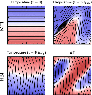
Illustration of the linear development of buoyancy instabilities in dilute plasmas from two-dimensional numerical simulations. Colour shows the temperature, increasing from blue to red, while black lines trace the magnetic field. Top row: quasi-linear evolution of the MTI. Left-hand panel: initial equilibrium state, with  and the conductive heat flux Q = 0 everywhere. Right-hand panel: the plasma at t = 5tbuoy given an initial perturbation with
  . Flux freezing and rapid conduction along field lines ensure that Lagrangian fluid displacements are nearly isothermal. If the initial state has a positive temperature gradient, upwardly displaced fluid elements are warmer than their surroundings; they will expand and continue to rise. Similarly, downwardly displaced fluid elements are cooler than their surroundings and will sink. Bottom row: quasi-linear evolution of the HBI. The initial equilibrium state has
  and a net downward conductive heat flux, with ∇ · Q = 0 everywhere. Left-hand panel: the plasma at t = 5tbuoy given an initial perturbation with kx=kz. The perturbation alters the geometry of the magnetic field, so that field lines are not parallel and there can be conductive heating and cooling of the plasma. Right-hand panel: temperature difference at t = 5tbuoy relative to the initial condition. Magnetic field lines converge in upwardly displaced fluid elements, leading to an increased temperature. These fluid elements will then expand and continue to rise. Similarly, downwardly displaced fluid elements are conductively cooled, then they contract and continue to sink.
Quataert (2008) investigated the limit in which the temperature of the plasma increases with height. The instability in this case is known as the heat-flux-driven buoyancy instability, or HBI. We sketch the growth of the HBI in the bottom row of Fig. 1. Here, the initial equilibrium state has vertical magnetic field lines and a constant heat flux; the latter is required for the plasma to be in thermal equilibrium. However, perturbations to the magnetic field divert the heat flux and conductively heat or cool pockets of the plasma. If the temperature increases with height, upwardly displaced fluid elements become warmer than their surroundings and therefore experience a destabilizing buoyant response. These perturbations grow at the same rate |g ∂ ln T/∂z|1/2 as the MTI.
 , threaded by a constant magnetic field with any orientation in the
  plane:
 is the direction of the wave vector and
As we stated in Section 2.1, the growth rate in the rapid conduction limit is independent of thermal conductivity.
Equation (7) shows that magnetic tension can suppress the MTI and HBI; if ω2A > ω2buoy, p2 must be negative, and the plasma is stable to small perturbations. This is intuitively reasonable from Fig. 1: a strong magnetic field will resist the displacements shown there. In this paper, we focus on the relatively weak field limit in which magnetic tension does not suppress the instabilities, and we take ωA≪ωbuoy in equation (7). The dominant role of the magnetic field in our analysis is to enforce anisotropic electron heat transport.
For any magnetic field direction  , the term in square brackets in equation (7) can be positive or negative; thus, there are always linearly unstable modes, irrespective of the thermal state of the plasma (excluding the singular case of ∂T/∂z = 0).
We finally note that, although we neglected cooling in equation (1d), it adds a term to equation (7) which is insignificant when the cooling time is much longer than ω−1κ (Balbus & Reynolds 2008, 2010). This is not necessarily the case near the centres of cool-core clusters, and we plan to explore the combined effects of cooling and buoyancy instabilities in future work. For now, we assume that the buoyancy instabilities develop independently of cooling; this allows us to understand the non-linear development and saturation of the instabilities themselves and therefore to assess their possible implications for the thermal balance of the plasma.
3 NUMERICAL METHOD
3.1 Problem set-up and integration
We consider the evolution of a volume of plasma initially in hydrostatic and thermal equilibrium, but subject to either the HBI or MTI. We seed our simulations with Gaussian-random velocity perturbations with a flat spatial power spectrum and a standard deviation of 10−4cs. The small amplitude of these initial perturbations ensures that the instabilities begin in a linear phase and permits us to compare our results with the predictions of equation (7). Astrophysical perturbations are unlikely to be this subsonic, however, and the instabilities in our simulations take much longer to saturate than one would expect from the larger perturbations found in a more realistic scenario. We return to this point in Section 6.
We highlight the distinctness of the HBI and MTI from adiabatic convection by choosing initial conditions with ∂s/∂z > 0 whenever possible, so that the plasma would be absolutely stable if it were adiabatic. Our results do not rely critically on this choice, however, because the plasma is not adiabatic and its evolution is independent of its entropy gradient to the lowest order in ωbuoy/ωκ. Our results are much easier to interpret when ωbuoy does not vary across the simulation domain, and we prioritize this constraint on the initial condition over the sign of its entropy gradient (as we discuss in more detail below).
We solve equations (1a)–(1c), along with a conservative form of equation (1d), using the conservative MHD code Athena (Gardiner & Stone 2008; Stone et al. 2008) with the anisotropic conduction algorithm described in Parrish & Stone (2005) and Sharma & Hammett (2007). In particular, we use the monotonized central difference limiter on transverse heat fluxes to ensure stability. This conduction algorithm is subcycled with respect to the main integrator with a time-step Δt∝ (Δx)2; our simulations are therefore more computationally expensive than adiabatic MHD calculations. We draw most of our conclusions from simulations performed on uniform Cartesian grids of (64)3 and (128)3 cells. We also performed a large number of two-dimensional simulations on grids of (64)2, (128)2 and (256)2.
We perform our calculations in the plane-parallel approximation with a uniform gravity  . We fix the temperature at the upper and lower boundaries of our computational domain, and we extrapolate the pressure into the upper and lower ghost cells to enforce hydrostatic equilibrium at the boundary. For all other plasma variables, we apply reflecting boundary conditions in the direction parallel to gravity and periodic boundary conditions in the orthogonal directions. As we discuss in Section 4, the choice of fixed temperatures at the upper and lower boundaries has an important effect on the non-linear evolution. Simulations with Neumann boundary conditions in which the temperature at the boundaries is free to adjust would give somewhat different results (see e.g. Parrish & Stone 2005). Our choice of Dirichlet boundary conditions is motivated largely by the fact that many galaxy clusters in the local universe are observed to have non-negligible temperature gradients (Piffaretti et al. 2005).
We perform both local (with the size of the simulation domain L being much smaller than the scale-height H) and global (L≳H) simulations of the MTI and HBI. The local simulations separate the development of the instability from any large-scale response of the plasma, allowing us to study the dynamics in great detail. However, because the response of the plasma on larger scales can influence the non-linear evolution and saturation of the instabilities, we also carry out global simulations. We detail our initial conditions for these simulations in the following sections.
3.2 Local simulations
Both of the above atmospheres have positive entropy gradients and therefore would be stable in the absence of anisotropic conduction. The results we describe in this paper are entirely due to non-adiabatic processes.
We show in Section 4.1 that local and global HBI simulations give very similar results; we therefore use the simpler, local simulations for most of our analysis of the HBI. By contrast, the large-scale vertical motions induced by MTI make its evolution inherently global; as we describe in Section 4.2, local simulations do not give a converged result independent of L/H. We therefore study the saturated state of the MTI using global simulations, which require an alternative set of initial conditions.
3.3 Global simulations

The positive and negative signs in equation (10b) produce atmospheres unstable to the HBI and MTI, respectively. Note that T(z = 0) = 1 as in our local simulations. We take g0 = 1, S = 3 and ω2buoy = 1/2 and numerically solve for ρ(z) so that the initial atmosphere is in hydrostatic equilibrium. The atmosphere defined by equation (10) does not have a single, well-defined scale-height. We therefore define H so that L/H = ln (Tmax/Tmin); this definition for H is analogous to that used in our local simulations and L/H reflects the total free energy available to the instabilities. Because H is a defined, rather than fundamental, property of the atmosphere, it is not independent of the size of the simulation domain. We carry out simulations with domain sizes L = 0.5 and 2.0, which have L/H = 0.27 and 1.4, respectively.
Simulations with a larger simulation domain size inherently permit larger vertical displacements, and the boundary conditions do not influence the evolution of the plasma as strongly as they do in a local simulation. We find that the neutrally stable layers described in Section 3.2 do not alter the results of our global simulations, and we therefore do not include them in our global set-up.
We chose the conductivity in our local simulations so that κe = 10ρωbuoyL2, but the corresponding constraint on the time-step becomes impractical for our global simulations. Instead, we adjust κe so that the ratio κe/L is the same as it is in the local simulations. This keeps the ratio of the conduction time to the sound-crossing time constant, and is appropriate if the turbulence driven by the MTI or HBI reaches a terminal speed less than or of the order of sound speed. We carried out simulations with different values of the conductivity and verified that our results are insensitive to order unity changes in κe.
The atmosphere we use for our global MTI simulations has a negative entropy gradient. One might worry that the results of these simulations – which aim to focus on the MTI – would be biased by the presence of adiabatic convection. This is only a pedagogical inconvenience, however; ωκ > N on all relevant scales in the simulation, so the adiabatic limit to equation (4) is not important, and the evolution of the plasma is nearly independent of its entropy gradient. To confirm this we carried out L = 0.27 H simulations with both sets of initial conditions; they give very similar results. Additionally, we performed one simulation of adiabatic convection using this set-up, and the behaviour of this simulation is entirely different from that of our MTI simulations: after a brief period of convection, the atmosphere rapidly became isentropic and settled into a quiescent state.
3.4 Turbulence
The pure HBI/MTI simulations described in the previous sections are physically very instructive but astrophysically somewhat idealized. In order to better understand the astrophysical role of the HBI and MTI, we also study their interaction with other sources of turbulence and fluid motion. We assume that these take the form of isotropic turbulence, which we include via the externally imposed force field f in equation (1b). Following Lemaster & Stone (2008), we compute f in momentum space from scales k0={4, 6, 8}× 2 π/L, down to kmax = 2k0, with an injected energy spectrum  . We then randomize the phases, perform a Helmholtz decomposition of the field, discard the compressive component, transform the field into configuration space and normalize it to a specified energy injection rate. We find that the turbulence sets up a non-linear cascade that is not very sensitive to either the driving scale or the injected spectrum of the turbulence.
This prescription for turbulence is statistically uniform in both space and time and therefore provides a controlled environment in which to study the interaction between turbulence and buoyancy instabilities. This may not, however, be a good approximation to real astrophysical turbulence; we discuss the implications of our choice in Sections 5 and 6.
3.5 Convergence
We found that the kinetic energy and mean magnetic field angles in our local HBI simulations converge by a resolution of (64)3 cells, and that our global HBI simulations converge with roughly 60 grid cells per scale-height. Convergence is more subtle in our MTI simulations, however. We performed our global MTI simulation on grids of (64)3, (96)3 and (128)3 cells and found that the saturated kinetic energies agree to within 5 per cent and show no trend with resolution. We also performed a simulation on a grid of (256)3 cells and found, surprisingly, that the saturated kinetic energy in this simulation is lower by about 15 per cent. Unfortunately, we are unable to say whether this is indicative of a trend at higher resolution, as a yet higher resolution simulation would be extremely computationally expensive given the short Courant time-scale associated with the thermal conduction.
Experience with the magnetorotational instability (MRI; Balbus & Hawley 1991) shows that convergence in turbulent MHD simulations can be quite subtle (see Fromang & Papaloizou 2007; Davis, Stone & Pessah 2010), but it is unclear as to what extent these lessons apply to the MTI. For example, the MTI is much more weakly sensitive to the lack of a net magnetic flux (Parrish & Stone 2007). None the less, a more detailed convergence study will be necessary to fully understand the saturation of the MTI.
We finally note that all viscous and magnetic dissipation in our simulations is numerical; specifically, we have not controlled either the Prandtl or the magnetic Prandtl numbers. MHD turbulence can be sensitive to these quantities, but we leave a thorough parameter study to future work.
4 NON-LINEAR SATURATION
4.1 Saturation of the HBI
Parrish & Quataert (2008) described the non-linear saturation of the HBI, but they did not explicitly test the dependence of their results on the size of the computational domain. This dependence turns out to be crucial for the MTI (see Section 4.2), but we show here that the size of the domain has little effect on the saturation of the HBI. None the less, we describe the non-linear behaviour of the HBI in reasonable detail, expanding on the physical interpretation given in previous papers (although our HBI results do not differ significantly from those of previous authors). The saturation of the HBI is the simplest process we consider in this paper and will serve as a useful comparison for our new results.
We study the saturation of the HBI using 2D and 3D simulations spanning a range of domain sizes L/H. Table 1 lists all of the simulations presented in this section.
Parameters for HBI simulations (Section 4.1).
| Name | D | res | L/H | κ |
| h1 | 2 | 64 | 0.05 | 7.07 |
| h2 | 3 | 64 | 0.05 | 7.07 |
| h3 | 3 | 128 | 0.75 | 0.47 |
| h4 | 3 | 128 | 1.40 | 0.35 |
| Name | D | res | L/H | κ |
| h1 | 2 | 64 | 0.05 | 7.07 |
| h2 | 3 | 64 | 0.05 | 7.07 |
| h3 | 3 | 128 | 0.75 | 0.47 |
| h4 | 3 | 128 | 1.40 | 0.35 |
All simulations are performed on square Cartesian grids of size L. D is the dimensionality of the simulation, res is the number of grid cells along a side, and κ is the conductivity (in units of kB/μm×ρωbuoyL2). All of these simulations are local (equation 8), except for the one with L/H = 1.4, which uses the global set-up (equation 10). We initialized all of these simulations with weak horizontal magnetic fields ( ).
).
Parameters for HBI simulations (Section 4.1).
| Name | D | res | L/H | κ |
| h1 | 2 | 64 | 0.05 | 7.07 |
| h2 | 3 | 64 | 0.05 | 7.07 |
| h3 | 3 | 128 | 0.75 | 0.47 |
| h4 | 3 | 128 | 1.40 | 0.35 |
| Name | D | res | L/H | κ |
| h1 | 2 | 64 | 0.05 | 7.07 |
| h2 | 3 | 64 | 0.05 | 7.07 |
| h3 | 3 | 128 | 0.75 | 0.47 |
| h4 | 3 | 128 | 1.40 | 0.35 |
All simulations are performed on square Cartesian grids of size L. D is the dimensionality of the simulation, res is the number of grid cells along a side, and κ is the conductivity (in units of kB/μm×ρωbuoyL2). All of these simulations are local (equation 8), except for the one with L/H = 1.4, which uses the global set-up (equation 10). We initialized all of these simulations with weak horizontal magnetic fields ().
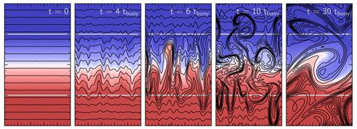
Fig. 2 shows snapshots of the evolution of temperature and magnetic field lines in a local, 2D HBI simulation. We chose this simulation to simplify the field-line visualization, but the results in Fig. 2 apply equally to our local and global 3D simulations. We initialized this simulation in an unstable equilibrium state with vertical magnetic field lines ( ). As described in Section 3.1, we seed this initial condition with small velocity perturbations; the HBI causes these perturbations to grow in the first three panels of Fig. 2. The evolution becomes non-linear in the third panel, when the velocity perturbations reach ∼4 per cent of the sound speed. Afterwards, the instability begins to saturate and the plasma slowly settles into a new equilibrium state. The last panel in Fig. 2 shows that this saturated state is highly anisotropic: the magnetic field lines are almost entirely orthogonal to gravity. Flux conservation implies that the fluid motions must also be anisotropic, with most of the kinetic energy in horizontal motions at late times (see Fig. 3, discussed below). These horizontal motions are very subsonic: in all of our simulations, the velocities generated by the HBI are significantly less than 1 per cent of the sound speed in the saturated state.
Evolution of the HBI with an initially vertical magnetic field in a local, 2D simulation (simulation h1 in Table 1). Colour shows temperature and black lines show magnetic field lines. A small velocity perturbation to the initial state seeds exponentially growing modes which dramatically reorient the magnetic field to be predominantly horizontal. The induced velocities are always highly subsonic and, after t∼ 20tbuoy, are also almost entirely horizontal. Once the plasma reaches its saturated state, it is buoyantly stable to vertical displacements. The plasma does not resist horizontal displacements, but the saturated state is nearly symmetric to these displacements and they do not change its character.
Evolution of the vertical and horizontal kinetic energy in a local, 2D HBI simulation (simulation h1 in Table 1). The units are such that the thermal pressure P≈ 1 and the initial magnetic energy is B2/8π = 10−12. After a period of exponential growth in which the x and z motions are in approximate equipartition, HBI saturates and the kinetic energy ceases to grow. At this point, the energy in the vertical motion is in the form of stable oscillations, which decay non-linearly. The horizontal motions are unhindered, however, and persist for the entire duration of the simulation. These horizontal motions are responsible for the asymmetry of the magnetic field shown in Fig. 4.
 ; these modes have the growth rate
 , only modes with
  are unstable. Since the HBI saturates by making the field lines horizontal (
 ), both the maximum growth rate of the instability and the volume of phase space for unstable modes decrease as the HBI develops. This strongly limits the growth of the perturbations, and helps explain why the instability saturates relatively quiescently.
As argued by Parrish & Quataert (2008), the HBI saturates when its maximum growth rate pmax vanishes, so that no unstable modes remain. While this is clearly a sufficient condition for the plasma to reach a new stable equilibrium, it is by no means necessary. The instability could, e.g. saturate via non-linear effects, but in practice this is not the case (at least for simulations without an additional source of turbulence; see Section 5.1). Equation (11) for pmax shows that the HBI can saturate by making either ∂T/∂z or  vanish; intuitively, the HBI is powered by a conductive heat flux, which it must extinguish in order to stop growing. Erasing the temperature gradient might seem like the more natural saturation channel, since the conduction time across the domain is much shorter than other time-scales in the problem. In an astrophysical setting, however, the large-scale temperature field is often controlled by cooling, accretion or other processes apart from the HBI. We therefore impose the overall temperature gradient on our simulations by fixing the temperature at the top and bottom of the domain, so that ωbuoy is roughly independent of time, and saturation requires
  .
.
 limit in equation (7) to understand the late-time behaviour of the plasma:
 which feels no restoring force. This simply reflects the fact that the plasma is stably stratified and resists vertical displacements. Displacements orthogonal to gravity are unaffected by buoyancy, however, and appear as zero-frequency modes in the dispersion relation.
Fig. 3 demonstrates this asymmetry between vertical and horizontal displacements in the late-time evolution of the plasma. This figure shows the kinetic energy in horizontal and vertical motions as a function of time. During the initial, linear growth of the instability (t≲ 10tbuoy), buoyantly unstable fluid elements accelerate towards the stable equilibrium, and the kinetic energy is approximately evenly split among vertical and horizontal motions. As the instability saturates, however, the plasma becomes buoyantly stable and traps the vertical motions in decaying oscillations (internal gravity waves). The horizontal motions keep going, however, and retain their kinetic energy for the duration of the simulation. This difference in the response of the plasma to vertical and horizontal motions accounts for the anisotropy of the velocity field in the saturated state of the HBI.
Fig. 4 shows the evolution of the rms magnetic field angle (left-hand panel) and magnetic energy (right-hand panel) in 3D HBI simulations for three different values of the size of the computational domain L relative to the scale-height H. The zero-frequency modes discussed above also dominate the evolution of the magnetic field at late times, after the motions become non-linear (t≳ 10tbuoy). The horizontal displacements stretch out the field lines, amplifying and reorienting them. Quantitatively, we expect that  , where λ is a characteristic scale for the modes in the saturated state, ξ is the magnitude of the horizontal displacements, and we have assumed that the velocity is constant with time. The left-hand panel of Fig. 4 shows that the dependence in the simulations is quite close to this, with
  .4 Stretching the field lines in this manner amplifies the field strength by the amount of δB∝ξ; if the velocity is constant with time, we expect B2∝t2. The right-hand panel of Fig. 4 shows that this time dependence is approximately true for our two larger HBI simulations; the amplification is slightly slower in the very local calculation with L/H = 0.05. There is no indication that the magnetic field amplification has saturated at late times in our HBI simulations. We suspect that the amplification would continue until the magnetic and kinetic energy densities reach approximate equipartition, but we would have to run the simulation for a very long time to confirm this.
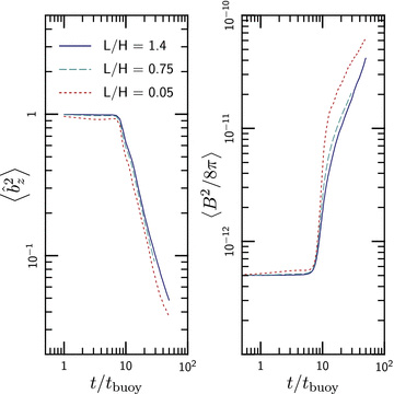
Evolution of the orientation (left) and energy (right) of the magnetic field in 3D HBI simulations for three different values of the size of simulation domain relative to the temperature scaleheight (L/H) (simulations h2–h4 in Table 1). Units are such that the thermal pressure P is ≃ 1. The results are nearly independent of size of the simulation domain. As described in Section 4.1, the HBI saturates by shutting itself off; the linear exponential growth ends at t∼ 10tbuoy, and most of the evolution of the magnetic field happens afterwards. This evolution is driven by the horizontal motions shown in Fig. 3, which both amplify and reorient the magnetic field. After a brief period of exponential growth, the field amplification is roughly linear in time. By contrast, the field amplification by the MTI is exponential in time (see Fig. 8).
One of the important results in Fig. 4 is that the saturated state of the HBI is nearly independent of the size of the computational domain L/H. Since the late-time evolution of the plasma is driven only by horizontal displacements, the key dynamics all occur at approximately the same height in the atmosphere. The saturation of the HBI is thus essentially local in nature and should not be sensitive to the global thermal state of the plasma or the details of the computational set-up.
The dramatic reorienting of the magnetic field caused by the HBI severely suppresses the conductive heat flux through the plasma. The conductive flux is proportional to  , which decreases in time ∝ (t/tbuoy)−1.7. The saturated state of the HBI is also buoyantly stable and resists any vertical mixing of the plasma. As a result, the convective energy fluxes in our HBI simulations are very small, ∼10−6 ρc3s. The effect of the HBI therefore is to strongly insulate the plasma against both conductive and convective energy transport. This can dramatically affect the thermal evolution of the plasma (Bogdanović et al. 2009; Parrish et al. 2009).
The fact that the growth rate of the HBI depends on the local orientation of the magnetic field, as well as the thermal structure of the plasma, makes it very different from adiabatic convection. This dependence on the magnetic field structure provides a saturation channel in which the kinetic energies are very small compared to the thermal energy (e.g. in Fig. 3, ρv2/nkT∼ 10−5). Critically, these highly subsonic motions occur in simulations in which the boundary conditions allow for the presence of a sustained, order unity, temperature gradient (d ln T/d ln z∼ 1). In an adiabatic simulation, the analogous sustained entropy gradient would generate convective motions with ρv2∼nkT. This does not occur in an HBI-unstable plasma. Thus, although a plasma with a positive temperature gradient is in general buoyantly unstable, the effect of the HBI is to peacefully stabilize the plasma within a few buoyancy times by suppressing the conductive heat flux through the plasma. The resulting stably stratified plasma then resists vertical mixing and, in the absence of strong external forcing, we expect the fluid velocities and magnetic field lines to be primarily horizontal. In Section 5, we perturb this state with externally driven, isotropic turbulence and test the strength of the stabilizing force.
4.2 Saturation of the MTI
Fig. 5 shows the evolution of one of our local, 2D MTI simulations. As in the HBI simulation shown in Fig. 2, we initialized this simulation in an unstable equilibrium state (a weak horizontal magnetic field) and seeded it with the small velocity perturbations described in Section 3.1. The MTI and HBI stem from very similar physics, and as a result have very similar linear dynamics. The non-linear behaviour of the two instabilities is entirely different, however. While the HBI saturates relatively quiescently by driving the plasma to a buoyantly stable and highly anisotropic state, the MTI generates vigorous, sustained convection that tends to isotropize both the magnetic and velocity fields.
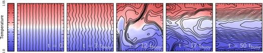
Evolution of the MTI with an initially horizontal magnetic field in a local, 2D simulation (simulation m1 in Table 2). Grey horizontal lines show the transition to the buoyantly neutral layers described in Section 3.2; the colour scale is identical to that in Fig. 2. Initial perturbations grow by the mechanism described in Section 2.2 (Fig. 1); rising and sinking plumes rake out the field lines until, by t = 6tbuoy, they are mostly vertical. This configuration is, however, non-linearly unstable to horizontal displacements, which generate a horizontal magnetic field and thus continually seed the MTI (see Fig. 6). The result is vigorous, sustained convection in marked contrast to the saturation of the HBI in Fig. 2. In this local simulation, buoyant plumes accelerate until they reach the neutrally stable layers. The boundaries prematurely stop the growth of the MTI, and the local simulation underpredicts the kinetic energy generated by the MTI (see Fig. 7).
As we did for the HBI, we study the saturation of the MTI using 2D and 3D simulations spanning a range of domain sizes L/H. Table 2 summarizes the simulations presented in this section.
Parameters for MTI simulations (Section 4.2).
| Name | D | res | L/H | κ | Field configuration |
| m1 | 2 | 64 | 0.033 | 7.07 | horizontal |
| m2 | 2 | 64 | 0.033 | 7.07 | vertical |
| m3 | 3 | 64 | 0.033 | 7.07 | horizontal |
| m4 | 3 | 64 | 0.033 | 7.07 | vertical |
| m5* | 3 | 128 | 0.500 | 0.31 | horizontal |
| m6* | 3 | 128 | 1.400 | 0.35 | horizontal |
| m7 | 3 | 256 | 0.500 | 0.06 | horizontal |
The definitions of L, D, and κ are the same as in Table 1. All simulations use the local set-up (equation 9), except for the one with L/H = 1.4, which is global (equation 10). Each of these simulations was initialized with a weak magnetic field  with the orientation indicated in the table.
*We also repeated simulations m5 and m6 with initial field strengths  .
.
Parameters for MTI simulations (Section 4.2).
| Name | D | res | L/H | κ | Field configuration |
| m1 | 2 | 64 | 0.033 | 7.07 | horizontal |
| m2 | 2 | 64 | 0.033 | 7.07 | vertical |
| m3 | 3 | 64 | 0.033 | 7.07 | horizontal |
| m4 | 3 | 64 | 0.033 | 7.07 | vertical |
| m5* | 3 | 128 | 0.500 | 0.31 | horizontal |
| m6* | 3 | 128 | 1.400 | 0.35 | horizontal |
| m7 | 3 | 256 | 0.500 | 0.06 | horizontal |
| Name | D | res | L/H | κ | Field configuration |
| m1 | 2 | 64 | 0.033 | 7.07 | horizontal |
| m2 | 2 | 64 | 0.033 | 7.07 | vertical |
| m3 | 3 | 64 | 0.033 | 7.07 | horizontal |
| m4 | 3 | 64 | 0.033 | 7.07 | vertical |
| m5* | 3 | 128 | 0.500 | 0.31 | horizontal |
| m6* | 3 | 128 | 1.400 | 0.35 | horizontal |
| m7 | 3 | 256 | 0.500 | 0.06 | horizontal |
The definitions of L, D, and κ are the same as in Table 1. All simulations use the local set-up (equation 9), except for the one with L/H = 1.4, which is global (equation 10). Each of these simulations was initialized with a weak magnetic field with the orientation indicated in the table.
*We also repeated simulations m5 and m6 with initial field strengths .
Since the linear dispersion relation successfully describes the non-linear evolution and saturation of the HBI, it is a good place to begin our discussion of the MTI. The MTI is described by equation (7) when ∂T/∂z < 0. The linear evolution of the MTI is the opposite of that of the HBI: the MTI operates when the temperature decreases with height, its fastest growing modes are the ones with wave vectors k parallel to  , and the force that destabilizes the MTI is exactly that which stabilizes the HBI in its saturated state. Equation (7) shows that the maximum growth rate of the MTI goes to zero when
  . By analogy with the HBI, it thus seems reasonable to expect that the MTI also saturates quiescently, by making the field lines vertical.
The first three panels of Fig. 5 show that this is nearly what happens. As the perturbations grow exponentially, the buoyantly rising and sinking blobs rake out the field lines, making them largely vertical. The growth rate of the MTI goes to zero when the field lines become vertical; since the velocities are still small at this point in the evolution (∼10−2cs), one might expect the MTI to operate like the HBI and quiescently settle into this stable equilibrium state. Instead, however, the MTI drives sustained turbulence for as long as the temperature gradient persists. The plasma never becomes buoyantly stable, and the magnetic field and fluid velocities are nearly isotropic at late times.
We can understand this evolution using the same approach we employed for the HBI. Although the plasma in our MTI simulations never reaches a state in which the MTI growth rate is zero, examining the properties of this state is very instructive. The equilibrium state of the MTI with  (i.e. a vertical field) has precisely the same dispersion relation as the saturated state of the HBI, given by equation (12). There are again zero-frequency (neutrally stable) modes of the dispersion relation which correspond to horizontal perturbations to the equilibrium state of the MTI; these experience no restoring force, because the restoring force is buoyant in nature and unaffected by horizontal displacements.5 Critically, however, these zero-frequency perturbations now add a horizontal component to the magnetic field, pulling the plasma out of the equilibrium state and rendering it unstable to the MTI.
Fig. 6 vividly illustrates this process. This figure shows a simulation that starts with the linearly stable equilibrium state of the MTI (a vertical magnetic field), seeded with the same highly subsonic velocity perturbations as before. The compressive component of the perturbation rapidly damps because the Mach number is small, and buoyancy traps the vertical components of the perturbation in small-amplitude oscillations, as predicted by equation (12). The incompressive, horizontal displacements propagate freely, however, and by t = 7.5tbuoy, they have noticeably changed the local orientation of the magnetic field. The plasma is no longer in its stable equilibrium state, and by t = 20tbuoy, it is clear that this process has excited the MTI. At late times, the simulations initialized with horizontal (linearly unstable; Fig. 5) and vertical (linearly stable; Fig. 6) magnetic fields are qualitatively indistinguishable. Thus, although equation (7) shows that a plasma with ∂T/∂z < 0 is linearly stable if the magnetic field is vertical, that configuration is non-linearly unstable.
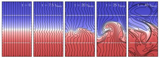
Evolution of the MTI in a plasma with an initially vertical magnetic field in a local, 2D simulation (simulation m2 in Table 2). This configuration is linearly stable according to equation (7), but there are zero-frequency, kx = 0, modes which do not have a restoring force. Physically, these correspond to horizontal motions which do not feel gravity/buoyancy. Because of these zero-frequency modes, small random initial perturbations add a horizontal component to the magnetic field, eventually rendering the plasma unstable to the MTI. This creates a feedback loop, allowing the MTI to generate vigorous, sustained convection; the HBI does not have this same feedback loop and so does not generate sustained turbulence (Fig. 2). At late times, the results of this simulation with an initially vertical magnetic field are very similar to Fig. 5 which starts with a horizontal magnetic field.
The non-linear instability of the  state of the MTI precludes the magnetic saturation channel. The zero-frequency horizontal motions generate a horizontal magnetic field component from the vertical magnetic field, seeding the instability and closing the dynamo loop. This continuously drives the MTI and generates sustained turbulence. Without a linear means to saturate, the MTI grows until non-linear effects can compete with the linear instability, which requires v∼cs.
Fig. 7 shows the Mach number in 3D MTI simulations as a function of time, for different sizes of the computational domain L/H. The MTI buoyantly accelerates rising or sinking fluid elements. For simulations with L≪H, the velocities generated by the MTI are artificially suppressed because the small size of the computational domain prematurely stops the buoyant acceleration (Fig. 5). Fig. 7 shows that the results of these simulations are reasonably consistent with mixing length estimate  . By contrast, for simulations with L≳H, the Mach numbers approach ∼1 so that the MTI taps into the full buoyant force associated with the unstable temperature gradient. This is only true, of course, because our boundary conditions fix the temperature at the top and bottom of the computational domain. If the temperatures were free to vary, the MTI could saturate by making the plasma isothermal. Which of these saturation mechanisms is realized in a given astrophysical system will depend on the heating and cooling mechanisms that regulate the temperature profile of the plasma.
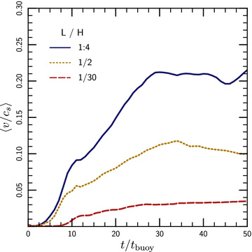
Volume-averaged Mach numbers of the turbulence generated by MTI in 3D simulations, for three different values of the size of simulation domain relative to the temperature scaleheight L/H. MTI buoyantly accelerates the unstable fluid elements; if the size of the simulation domain is smaller than a scaleheight, the boundaries suppress the growth of the instability. Local simulations with L/H = 1/30 therefore strongly underpredict the strength of the turbulence generated by MTI. In global simulations with L≳H, MTI leads to turbulence with average Mach numbers of ∼0.2; the velocity distribution extends up to ∼5 times the mean.
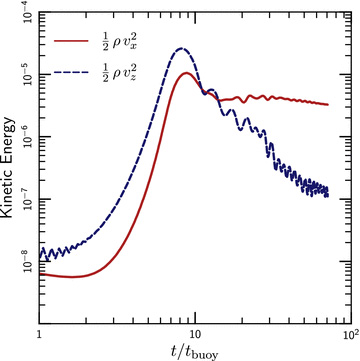
Fig. 8 shows the evolution of the magnetic field orientation (left-hand panel) and energy (right-hand panel) as a function of time in our 3D MTI simulations (for two different values of L/H). The sustained, vigorous turbulence generated by the MTI in the non-linear regime (t≳ 10tbuoy) rapidly amplifies the magnetic field. The magnetic and kinetic energies reach approximate equipartition in our simulations, with B2/8π∼ 0.1ρv2. The kinetic and magnetic energies generated by the MTI together contribute ∼5–10 per cent of the pressure support in its saturated state.

Left-hand panel: evolution of the magnetic field orientation in 3D MTI simulations, for two different values of the size of simulation domain relative to the temperature scaleheight L/H. During the linear phase of evolution (t≲ 10tbuoy), the MTI drives the plasma towards a nearly vertical magnetic field, i.e.  . When the instability becomes non-linear, however (near t∼ 10tbuoy), the evolution changes. Unlike the HBI, the plasma never settles into an equilibrium state; instead the MTI drives vigorous turbulence. This turbulence amplifies and nearly isotropizes the magnetic field. Right-hand panel: evolution of the magnetic (dashed line) and kinetic (solid line) energy in local (L/H = 1/2) 3D MTI simulations, with different initial field strengths. These local simulations have a positive entropy gradient, but underpredict the magnetic and kinetic energy produced by the MTI. The magnetic energy in the saturated state approaches ∼10 per cent ×ρv2.
The evolution of the magnetic field geometry, shown in the left-hand panel of Fig. 8, nicely illustrates the transition of the MTI from the linear to the non-linear regime. During the linear phase of the instability (t≲ 10tbuoy), the plasma accelerates towards the equilibrium state with  . After the evolution becomes non-linear (t≳ 10tbuoy), however, the MTI drives sustained turbulence, which nearly isotropizes the magnetic field.
While the HBI works to insulate the plasma against vertical energy transport, the MTI enhances it. Fig. 8 shows that the conductive flux through the plasma is slightly greater than ∼1/3 of the field-free value κe∇T[because  ]. Moreover, the MTI leads to large fluid velocities and correlated temperature and velocity perturbations – hot pockets of plasma rise, while cool pockets sink. These imply that the MTI drives an efficient outwards convective heat flux. Fig. 9 shows that this flux can be ∼1.5 per cent of ρc3s, consistent with the Mach numbers of ∼0.2 in Fig. 7. This convective flux is probably not large enough to influence the thermodynamics of the ICM, but it could be important in other environments where the MTI can operate, such as the interiors of white dwarfs and neutron stars (Chang & Quataert 2010).
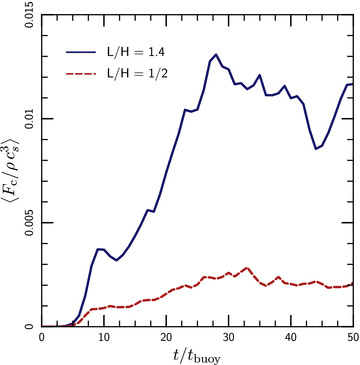
Convective energy fluxes generated by the MTI. The large turbulent velocities associated with the MTI (Fig. 7) lead to efficient convective transport of energy, at a reasonable fraction of the maximal value, ρc3s. In these MTI simulations, the conductive energy flux is ∼0.4 times the field-free value and always dominates the convective energy flux for galaxy cluster conditions.
We close this section by noting a few details in our description of the MTI that have been glossed over. Though we call the simulation set-up shown in Fig. 6 linearly stable, this is only exactly true in the rapid-conduction limit. Balbus & Reynolds (2010) found that the plasma in this set-up is buoyantly overstable, with a growth time tgrow∼ 3tbuoy ωκ/ωbuoy∼ 20tbuoy. This time-scale is long compared to the growth we observe, however, and our results are consistent with the interpretation that the plasma is non-linearly unstable. We also note that the zero-frequency modes we describe actually have a finite frequency due to the restoring force of magnetic tension. This is very small in our simulations, however. Magnetic tension can, of course, stabilize this state if the magnetic field is strong enough. As mentioned in Section 2.2, however, we choose not to explore that limit.
5 INTERACTION WITH OTHER SOURCES OF TURBULENCE
Thus far, we have described the development and saturation of buoyancy instabilities only in the idealized case of an otherwise quiescent plasma. In a more astrophysically realistic scenario, however, other processes and sources of turbulence may also act on the plasma and the resulting dynamics can be more complicated. For example, the evolution of the HBI will not simply proceed until its growth rate is zero everywhere. Instead, we expect the saturated state to involve a statistical balance among the various forces; this balance depends on the buoyant properties of the plasma and provides a test of our understanding of the non-linear behaviour of the HBI and MTI. Furthermore, any change in the saturated state of the plasma due to the interaction between the HBI/MTI and other sources of turbulence could change the astrophysical implications of these instabilities.
We choose to explore the interaction between buoyancy instabilities and other sources of turbulence using the idealized, isotropic turbulence model described in Section 3.4. While this model glosses over the details of what generates the turbulence, we hope that it captures the essential physics of the problem, allowing us to study the effect of turbulence without unnecessarily restricting our analysis to specific applications. We intend to specialize to specific sources of turbulence in future work, but our present analysis should apply in the ICM, accretion discs, and anywhere else the assumptions summarized in Section 2.2 apply.
In the following sections, we study the transition from a state dominated by buoyancy to one dominated by isotropic turbulence using a number of simulations of the HBI and MTI, with turbulence in the range of 0.1 ≲tbuoy/tdist≲ 10.
5.1 Effect of turbulence on the HBI
Fig. 10 shows representative snapshots of the temperature and magnetic field lines in the saturated states of our HBI simulations with turbulence; the strength of the injected turbulence increases from the top left panel through the bottom right (the labels correspond to the values of tbuoy/tdist). When tdist is long compared to the buoyancy time, as in the first panel of Fig. 10, the turbulence is weak; the HBI therefore dominates and the evolution of the plasma is similar to that described in Section 4.1. The saturated state of the HBI feels a buoyant restoring force which resists vertical displacements ξz with a force per unit mass fbuoy=ω2buoyξz. As we increase the strength of the applied turbulence in the following panels of Fig. 10, the vertical displacements grow, and the field deviates more strongly from the  equilibrium state of the HBI. When tdist is short compared to the buoyancy time, as in the last panel of Fig. 10, turbulence can displace the fluid elements faster than buoyancy can restore them. The turbulence then dominates the evolution of the plasma, tangling and isotropizing the field lines.
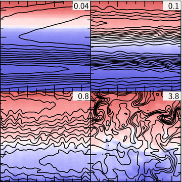
Snapshots of the saturated states of our 2D HBI simulations with externally driven turbulence. Colours show the temperature (increasing from blue to red), and black lines show magnetic field lines. Each panel is labelled with the dimensionless strength of the turbulence in the simulation, tbuoy/tdist, defined in Section 5. When tbuoy≲tdist, as in the top two panels, the HBI dominates the evolution of the plasma. When tbuoy≳tdist, the turbulence can isotropize the magnetic field, but it does so in a scale-dependent way with the large scales retaining memory of the horizontal field imposed by the HBI.
Fig. 10 also shows the length-scale dependence of the transition from an HBI to a turbulence-dominated state. It is clear in the second and third panels that the HBI has globally rearranged the field lines, but that the turbulence is increasingly efficient at smaller scales. This is a consequence of the fact that turbulence typically perturbs the plasma in a scale-dependent way, while the buoyant restoring force of the HBI does not. If the turbulence follows a Kolmogorov cascade, the force ∼ω2/k∝k1/3 increases with decreasing scale, so the turbulence will always win on sufficiently small length-scales. It is therefore somewhat ambiguous whether turbulence or the HBI dominates a certain configuration, as the answer will typically depend on scale. As mentioned earlier, we skirt this issue by defining tdist at the scale where the velocity spectrum of the injected turbulence peaks. When assessing the astrophysical importance of the HBI, it is important to keep this scale in mind. If the scale where the turbulent energy spectrum peaks is smaller than the temperature gradient length-scale, the HBI may still insulate the plasma against conduction, even if the field lines are isotropized on smaller scales.
In order to quantify the transition from an HBI-dominated configuration to one dominated by turbulence, we measure the mean orientation of the magnetic field via the volume average of  . The saturated value for this quantity approaches zero when the HBI dominates, and 1/D when the magnetic field is isotropic, where D is the number of dimensions in the simulation.
Fig. 11 shows the saturated field angle as a function of tbuoy/tdist. The points in this figure represent simulations with different driving scales k0, different dimensionality and different buoyancy times tbuoy (Table 3 summarizes our parameter study). Symmetry of the coordinate axes requires that b2z=1/2 in 2D or 1/3 in 3D if the magnetic field is isotropic. To include both our 2D and 3D simulations on the same plot, we shift our 3D values of 〈b2z〉 by a factor of 3/2. To within the scatter shown in Fig. 11, we find that the saturated value of 〈b2z〉 depends only on the ratio tbuoy/tdist: for tbuoy≳tdist the turbulence is strong and the field becomes relatively isotropic while for tbuoy≲tdist the isotropic turbulence is weak and the HBI drives the magnetic field to become relatively horizontal. The fact that the transition between these two states occurs around tbuoy∼tdist suggests that our definition of tdist, though somewhat arbitrary, is reasonable.
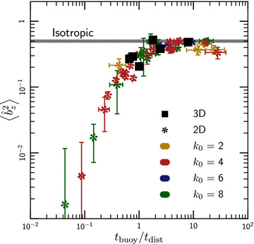
Saturated magnetic field orientation as a function of the strength of the externally driven turbulence, tbuoy/tdist, for local HBI unstable atmospheres with tbuoy = 1,  and
and  . The thick grey line is an isotropic magnetic field in 2D. Coloured points represent simulations with turbulence driven on different scales. Squares mark 3D calculations; the values of 〈b2z〉 for the 3D simulations have been shifted by a factor of 3/2 since isotropy implies b2z = 1/2 in 2D but b2z = 1/3 in 3D. Error bars represent 1σ statistical fluctuations in
  and tdist. These points are reasonably well fit by the broken power law
  .
.
Parameter study for HBI simulations with turbulence (Section 5.1).
| D (2) | res (64) | L (0.1) | H (2.0) | B0 (10−6) |  |
| – | – | – | – | – | 2 |
| – | – | – | 1.0 | – | 2 |
| – | – | – | 3.0 | – | 2 |
| – | – | – | – | – | 4 |
| – | – | 1.0 | – | – | 4 |
| – | – | 0.3 | – | – | 4 |
| 3 | – | – | – | – | 4 |
| 3 | – | – | – | 10−3 | 4 |
| 3 | – | 1.0 | – | 3 × 10⁻⁴ | 4 |
| 3 | 128 | 1.0 | – | 3 × 10⁻⁴ | 4 |
| – | – | – | – | – | 6 |
| – | – | – | – | – | 8 |
| – | 256 | – | – | – | 8 |
| 3 | – | – | – | – | 8 |
| D (2) | res (64) | L (0.1) | H (2.0) | B0 (10−6) | |
| – | – | – | – | – | 2 |
| – | – | – | 1.0 | – | 2 |
| – | – | – | 3.0 | – | 2 |
| – | – | – | – | – | 4 |
| – | – | 1.0 | – | – | 4 |
| – | – | 0.3 | – | – | 4 |
| 3 | – | – | – | – | 4 |
| 3 | – | – | – | 10−3 | 4 |
| 3 | – | 1.0 | – | 3 × 10⁻⁴ | 4 |
| 3 | 128 | 1.0 | – | 3 × 10⁻⁴ | 4 |
| – | – | – | – | – | 6 |
| – | – | – | – | – | 8 |
| – | 256 | – | – | – | 8 |
| 3 | – | – | – | – | 8 |
The simulations were initialized with our local set-up (equation 8) and an initial magnetic field strength B0. Each simulation was performed on uniform Cartesian grids of side L, resolution res and dimension D. We varied the size of the simulation domain L (scaling the conductivity as described in Section 3.3), the plasma scale-height H and the initial magnetic field strength B0; the fiducial values for these parameters are included in the table header (– indicates the fiducial value). For each entry in the table, we performed simulations with both initially horizontal and vertical magnetic fields. As described in Section 5.1, these simulations include isotropic turbulence injected on the scale  and with a range of turbulent energy injection rates to give 0.1 ≲tbuoy/tdist≲ 10.
Parameter study for HBI simulations with turbulence (Section 5.1).
| D (2) | res (64) | L (0.1) | H (2.0) | B0 (10−6) | |
| – | – | – | – | – | 2 |
| – | – | – | 1.0 | – | 2 |
| – | – | – | 3.0 | – | 2 |
| – | – | – | – | – | 4 |
| – | – | 1.0 | – | – | 4 |
| – | – | 0.3 | – | – | 4 |
| 3 | – | – | – | – | 4 |
| 3 | – | – | – | 10−3 | 4 |
| 3 | – | 1.0 | – | 3 × 10⁻⁴ | 4 |
| 3 | 128 | 1.0 | – | 3 × 10⁻⁴ | 4 |
| – | – | – | – | – | 6 |
| – | – | – | – | – | 8 |
| – | 256 | – | – | – | 8 |
| 3 | – | – | – | – | 8 |
The simulations were initialized with our local set-up (equation 8) and an initial magnetic field strength B0. Each simulation was performed on uniform Cartesian grids of side L, resolution res and dimension D. We varied the size of the simulation domain L (scaling the conductivity as described in Section 3.3), the plasma scale-height H and the initial magnetic field strength B0; the fiducial values for these parameters are included in the table header (– indicates the fiducial value). For each entry in the table, we performed simulations with both initially horizontal and vertical magnetic fields. As described in Section 5.1, these simulations include isotropic turbulence injected on the scale and with a range of turbulent energy injection rates to give 0.1 ≲tbuoy/tdist≲ 10.
The bulk of the simulations in Fig. 11 are 2D, and we do not have any 3D simulations in the very weak turbulence limit. These simulations are computationally expensive, both because of conduction and because we have to run them for a long time for turbulence and the HBI to reach a statistical steady state; using 2D simulations allowed us to explore a larger fraction of the interesting parameter space. While the development of turbulence is very different in two and three dimensions, the HBI is essentially two-dimensional in nature. Moreover, the key dynamics governing the interaction between the HBI and turbulence are dominated by the energy-containing scale of the turbulence – the precise power-spectrum of the fluctuations (which differs in 2D and 3D) is less critical. Scaling for dimension, we find that the saturated states of our 2D and 3D simulations are nearly identical. We thus believe that the results in Fig. 11 in the weak turbulence limit are a good description of the magnetic field structure in 3D systems as well.
These results on the interaction between the HBI and other sources of turbulence support an analogy between the saturated state of the HBI and ordinary, adiabatic stable stratification. The most important effect of the HBI in the saturated states of our simulations is to inhibit mixing in the direction of gravity. Ordinary stable stratification also inhibits vertical mixing and, as suggested by Sharma et al. (2009b), our parameter tbuoy/tdist is analogous to the Richardson number used in the hydrodynamics literature. To further expand on this analogy, Fig. 12 shows a comparison of anisotropically conducting (left-hand panel) and adiabatic (right-hand panel) simulations with equal values of tbuoy/tdist. For the adiabatic simulations, we define tbuoy=tad, i.e. using the entropy gradient rather than the temperature gradient. The left-hand panel of Fig. 12 shows simulations with the same injected turbulence, but initialized with vertical or horizontal magnetic field lines. In these simulations, the saturated state is independent of the initial condition. That is, the interaction between turbulence and the HBI leads to a well-defined magnetic field orientation that is independent of the initial field direction.
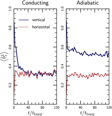
Magnetic field orientation as a function of time in 2D simulations with turbulence and the HBI for different initial magnetic field orientations; tbuoy/tdist = 0.8. Left-hand panel: simulations with anisotropic thermal conduction. Right-hand panel: adiabatic simulations with no conduction (and thus no HBI). Different curves represent simulations with initially vertical and horizontal magnetic field lines, respectively. Conducting simulations eventually reach the same saturated state independently of the initial magnetic field direction. Adiabatic simulations are very similar to the conducting ones if the field is initially horizontal, highlighting the fact that in the saturated state of HBI the plasma is buoyantly stable and behaves dynamically like an adiabatic fluid.
By contrast, in the adiabatic simulations (right-hand panel of Fig. 12), the final magnetic field orientation depends on the initial field direction. For an initially vertical field in an adiabatic plasma, the turbulence slowly isotropizes the magnetic field direction. However, the adiabatic simulations with initially horizontal field lines reach a saturated state that is very similar to that of the HBI simulations. In the adiabatic simulations, the magnetic field is essentially passive, but it traces the fluid displacements. The stable stratification competes with the turbulence and sets a typical scale for vertical displacements in the saturated state. This scale, in turn, determines the magnetic field geometry. The magnetic field plays no dynamical role in this process. The fact that the anisotropically conducting simulations reach the same statistical steady state highlights that the saturated state of the HBI behaves dynamically very much like an adiabatic, stably stratified plasma.
5.2 Effect of turbulence on the MTI
To complete our analysis, we study how externally imposed isotropic turbulence affects the saturation of the MTI. Fig. 13 shows the volume-averaged magnetic field orientation as a function of time in MTI simulations with additional turbulence, for different values of the strength of the turbulence tbuoy/tdist. These are local simulations [with domain sizes L/H = 0.5; initialized using equation (9)] which have the pedagogical advantage of a positive entropy gradient, but which underpredict the kinetic energy generated by the MTI. We drive the turbulence at relatively small scales (k L/2π = 8) so that subsonic turbulence can still satisfy tbuoy/tdist > 1. Both our driven turbulence and the MTI tend to isotropize the magnetic field, so it is not a priori clear whether the field orientation is a good indication of the importance of turbulence relative to the MTI. Although Fig. 13 shows that there is no strong dependence of the saturated field orientation on the strength of the turbulence, the time dependence of the field orientation clearly shows the effect of the turbulence on the MTI.
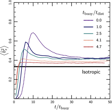
Magnetic field orientation as a function of time in 3D simulations with turbulence and the MTI, for different values of the strength of the turbulence tbuoy/tdist. In all of the simulations, the magnetic field is relatively isotropic in the saturated state. However, the early-time ‘overshoot’ towards a vertical magnetic field due to the MTI is suppressed in the presence of strong turbulence with tbuoy≳tdist. These relatively local simulations (L = 0.5H) underestimate the kinetic energy generated by the MTI (Fig. 7) and therefore the strength of the turbulence required to influence it.
In general, the evolution of the MTI proceeds through two stages: there is a linear phase, where the plasma accelerates towards its nominal stable state (which has a vertical magnetic field), and a non-linear transition to the saturated state, where the strong turbulence generated by the MTI isotropizes the velocities and field lines. In the absence of additional turbulence, the linear phase is characterized by field lines that are primarily in the direction of gravity (Fig. 5). Fig. 13 shows that additional sources of strong (rapidly shearing) turbulence suppress this linear phase of the MTI. Indeed, the evolution of the field angle with time in our strongest turbulence simulations (tbuoy/tdist = 4.7) is quite similar to what we find in simulations of an adiabatic plasma in which the MTI is not present.
It would, however, be incorrect to conclude from Fig. 13 that the MTI is unimportant if there are other strong sources of turbulence in the plasma. The fundamental reason for this is that the growth of the MTI does not depend significantly on scale, while the effects of the other sources of turbulence do. Fig. 14 shows the velocity spectra for the simulations in Fig. 13; for comparison we also show the velocity spectra in adiabatic simulations, which correspond to the power spectra produced solely by the injected turbulence. Fig. 13 demonstrates that even in simulations with very strong imposed turbulence (tbuoy/tdist = 4.7), there is still significant excess power on the largest scales in the computational domain (k L/2π≲ 10). This large-scale power is due to the MTI. Moreover, the turbulent energy due to the MTI dominates the total turbulent kinetic energy in the plasma. These results highlight that ‘strong’ turbulence is a scale-dependent statement. Suppressing the MTI requires having tbuoy/tdist≫ 1 on all scales, up to the temperature/pressure scaleheight of the plasma. Because the MTI itself generates nearly sonic velocities, this suppression would require close to supersonic turbulence. In practice, it is therefore unlikely that additional sources of turbulence can fully suppress the MTI in most astrophysical environments where it is likely to occur (e.g. accretion discs and galaxy clusters).
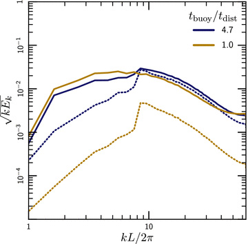
Velocity spectra in simulations with turbulence and the MTI (solid lines), for different values of the strength of the injected turbulence tbuoy/tdist. The turbulence is driven at k L/2π = 8. For comparison, dashed lines show the power spectra in adiabatic simulations, in which the injected turbulence is the only source of power. Even when tbuoy/tdist≫ 1 at the driving scale of the turbulence, so that one might expect the MTI to be suppressed, the MTI produces significant turbulent energy on larger scales k L/2π∼ 2−10. Suppressing the MTI on all scales in a plasma would thus require tbuoy/tdist≫ 1 on all scales smaller than the scale-height.
6 DISCUSSION
The motion of electrons along, but not across, magnetic field lines in dilute, magnetized plasmas produces efficient, anisotropic transport of heat. Such plasmas are therefore non-adiabatic, and the standard analysis of buoyancy (or convective) instabilities does not necessarily apply. Quantitatively, conduction plays an essential role on scales less than 7 (λH)1/2, where λ is the electron mean free path and H is the plasma scaleheight. In this ‘rapid conduction limit’, the temperature gradient, rather than the entropy gradient, dictates the stability of the plasma, and the plasma is unstable for either sign of the temperature gradient (Balbus 2000; Quataert 2008). The convective instability in this limit is known as the HBI (MTI) when the temperature increases (decreases) with height.
Parrish & Stone (2005, 2007) and Parrish & Quataert (2008) extended the original linear analysis of the MTI and HBI into the non-linear regime using numerical simulations. In this paper, we have reconsidered the non-linear saturation of the HBI and MTI. Our work adds to previous investigations because we have identified a key difference between the two instabilities and are able to understand the non-linear behaviour of the MTI more completely. This paper therefore represents a significant change in our understanding of the possible astrophysical implications of the MTI (but not HBI). We have also studied the effect of an external source of turbulence on both the MTI and the HBI. We conclude that other sources of turbulence in a plasma can change the saturation of the HBI, but that it is much harder to disrupt the MTI. Below we summarize our results and discuss their astrophysical implications, focusing on the intracluster medium (ICM) of galaxy clusters.
6.1 HBI
The HBI occurs whenever the temperature increases with height in an anisotropically conducting plasma. Plasmas in the rapid conduction limit are in general linearly unstable, unless the magnetic field lines are horizontal (equation 7). Horizontal field lines represent a fixed point in the evolution of the plasma: if the plasma somehow reaches such a state (and is not perturbed away by another process), it will remain there forever. A horizontal magnetic field is therefore a natural saturation channel for the HBI.
This ‘magnetic’ saturation mechanism can be understood using the linear dispersion relation of the plasma (Section 4.1). Starting from a linearly unstable state, the HBI induces both horizontal and vertical motions in the plasma. As the HBI develops, however, the vertical motions become trapped in internal gravity waves. These waves decay, leaving only the horizontal motions at late times; thus, the fluid velocities are very anisotropic in the saturated state. Since the horizontal motions do not incur a buoyant response, the horizontal displacements can be very large. These motions stretch out the magnetic field lines, amplifying and reorienting them, and drive the plasma towards its stable equilibrium with horizontal magnetic field lines. These horizontal motions therefore drive the non-linear evolution and saturation of the HBI.
Since the saturation of the HBI is dominated by horizontal displacements, the key dynamics all occur at approximately the same height in the atmosphere. The saturation of the HBI is thus essentially local in nature. We have demonstrated this explicitly by carrying out simulations with different domain sizes relative to the plasma scale-height; the results of these simulations are very similar (Fig. 4).
The growth rate of the HBI decreases dramatically as the instability progresses. The HBI therefore saturates quiescently, and the velocities in its saturated state are very subsonic (Fig. 3). The saturation is driven by horizontal motions with nearly constant velocities, so the non-linear magnetic field amplification is approximately linear, rather than exponential, with time. These findings are consistent with those of Parrish & Quataert (2008). We note that the HBI is very much unlike adiabatic convection, which can only saturate by changing the thermal state of the plasma and therefore generates vigorous turbulence. The key difference between the HBI and adiabatic convection is that the source of free energy for the HBI is a conductive heat flux through the plasma, not merely the existence of a temperature gradient. Since the heat flux can be suppressed by rearranging the magnetic field, the HBI has a magnetic saturation channel that is not available to adiabatic convection.
The astrophysical implications of the HBI follow immediately from the nature of its saturated state. By reorienting the magnetic field lines, the HBI dramatically reduces the conductive heat flux through the plasma. The HBI should operate in the innermost ∼100–200 kpc in the intracluster medium of cool-core galaxy clusters, where the observed temperature increases outward. As noted in Parrish & Quataert (2008), this is precisely where the cooling time of the ICM is shorter than its age; the HBI removes thermal conduction as a source of energy for the cores, potentially exacerbating the cooling flow problem (Parrish et al. 2009).
Our results demonstrate that the saturated state of the HBI is buoyantly stable. This may not seem surprising, because it is exactly what one would expect if the ICM were adiabatic. The ICM is not, however, adiabatic, and thermal conduction would render it buoyantly neutral to vertical displacements if the magnetic field lines were tangled. The saturated state of the HBI is buoyantly stable only because of the nearly horizontal magnetic field lines (that are perpendicular to the temperature gradient). The HBI therefore inhibits vertical mixing and allows for the existence of weakly damped internal gravity waves in the plasma.
Sharma et al. (2009b) noted that the stable stratification associated with the saturated state of the HBI competes with other sources of turbulence in a well-defined way. This competition can be understood using a modified Richardson number tbuoy/tdist, where tbuoy is the time-scale for the HBI to grow and tdist is a characteristic ‘distortion time’, or ‘eddy turnover time’, of the turbulence. When tbuoy≳tdist, the turbulence can isotropize the plasma and remove all traces of the HBI (Fig. 11). When tbuoy≲tdist, the saturated state of the plasma represents a statistical balance between turbulence and the HBI, with the magnetic field becoming more horizontal, and the plasma more HBI-dominated, for smaller values of tbuoy/tdist. The strength of other sources of turbulence is therefore crucial for understanding the astrophysical implications of the HBI.
Fig. 11 provides a very simple mapping between the properties of the turbulence and the magnetic field geometry in the plasma. Given the strength of the turbulence and the thermal state of the plasma, this figure provides a recipe for determining the mean geometry of the magnetic field, and therefore the effective conductivity of the plasma. This can be used to interpret observational results or to construct semi-analytic models of anisotropic conduction for use in cosmological simulations.
Turbulence in the ICM is currently poorly constrained, and thus it is difficult to determine precisely how important the HBI is for the evolution of clusters. Reasonable estimates suggest that tbuoy/tdist∼ 1, but more detailed simulations of clusters are required to determine this ratio more precisely. Future observations of the ICM with space-based X-ray calorimeters will place observational constraints on the level of turbulence. In addition, Faraday rotation measurements of the ICM will measure the orientation of the magnetic fields in clusters and constrain the role of the HBI (Bogdanović et al. 2010) (Pfrommer & Dursi 2010 describe another mechanism to measure the magnetic orientation in the ICM). Even if the turbulence is strong (tbuoy/tdist≳ 1), the driving scale and filling factor of the turbulence may allow the HBI to dominate on some scales or at some locations (see Fig. 10 and related discussions in Section 5.1). As suggested by Parrish et al. (2010) and Ruszkowski & Oh (2010), the interaction between turbulence and the HBI might be part of a feedback loop for the thermal evolution of the ICM.
6.2 MTI
The non-linear evolution of the MTI is more complex than that of the HBI. Just like the HBI, the MTI has linearly stable equilibria, but they are transposed: the linearly stable equilibrium states of the MTI have vertical field lines. We have shown, however, that the linearly stable equilibrium states turn out to be non-linearly unstable; i.e. they are unstable to perturbations with a finite amplitude. This non-linear instability arises because neutrally buoyant, horizontal displacements add a horizontal component to the magnetic field. This takes the plasma out of its linearly stable state and re-seeds the instability (Fig. 6 and Section 4.2). As a result, the linearly stable equilibrium states of the MTI do not represent fixed points in the evolution of the instability, and the MTI cannot saturate simply by reorienting the magnetic field.
This difference eliminates the quiescent, magnetic saturation channel for the MTI and dramatically changes its evolution. Without a linear means to saturate, the instability grows until non-linear effects dominate, which occurs when v∼cs. Unlike the HBI, the MTI therefore drives strong turbulence and operates as an efficient magnetic dynamo, much more akin to adiabatic convection. The astrophysical implications of the MTI are therefore entirely different from those of the HBI. The kinetic and magnetic energy generated by the MTI can contribute a significant (up to ten percent) non-thermal pressure support to the plasma in the saturated state. This is consistent with observational constraints on non-thermal pressure support in the ICM near the virial radius (George et al. 2009). This non-thermal pressure support may have consequences for mass estimates of clusters, which often rely on the assumption of hydrostatic equilibrium with thermal pressure support. Note, in particular, that the MTI is predicted to be present at precisely the same radii (≳ the scale radius) to which X-ray and SZ mass measurements are most sensitive.
Because the MTI operates by buoyantly accelerating fluid elements until they approach the sound speed, the results of numerical simulations of MTI are sensitive to the size of the computational domain. The boundaries of the domain can artificially suppress this acceleration, and simulations with sizes smaller than a scale-height underpredict the kinetic energy generated by the MTI (this was the case in the original MTI simulations of Parrish & Stone 2005, 2007). The non-linear development of the MTI is therefore quite sensitive to the global thermal state of the plasma, and an understanding of the MTI requires more careful numerical simulations than are needed for the HBI.
The saturated state of MTI corresponds to a largely isotropic magnetic field, with a slight but persistent vertical (or radial) bias; this bias is robust even in the presence of other sources of strong turbulence (Fig. 13). We find that the magnetic energy generated by the MTI saturates at about 30 per cent of the kinetic energy (Fig. 8). However, it may be difficult to observationally distinguish the turbulence generated by the MTI from that generated by other processes.
The large velocities generated by the MTI, along with correlations between the temperature and velocity perturbations, imply that the MTI drives a large convective heat flux, ∼1.5 per cent ×ρc3s (Fig. 9). While this convective flux is probably too small to alter the thermal evolution of the ICM, it could be important in higher-density astrophysical plasmas, where the electron mean free path is smaller and conduction is not as efficient.
While the MTI cannot saturate by reorienting the magnetic field, it can saturate by making the plasma isothermal. Simulations with Neumann boundary conditions in which the temperature at the boundaries is free to adjust find that this is the case; the atmosphere becomes isothermal before the MTI has a chance to develop (Parrish et al. 2008). We fixed the temperature at the top and bottom boundaries of our simulations; this is partially motivated by the fact that many galaxy clusters in the local universe are observed to have non-negligible temperature gradients.
Sharma et al. (2008) carried out numerical simulations of the MTI in spherical accretion flows and found nearly radial magnetic fields, with modest turbulence. This quasi-linear saturation of the MTI might seem to contradict the results presented in this paper. Note, however, that in the Bondi inflow studied by Sharma et al. (2008), the plasma undergoes at most ∼5–10 MTI growth times before flowing in. After 10 growth times, our simulations also show approximately radial field lines and modest turbulence (Fig. 8). Moreover, the simulations of Sharma et al. (2008) covered a very large dynamic range in radius and may have lacked the resolution to see the full non-linear development of the MTI.
The MTI growth time in the outer parts of the ICM is about 1 Gyr. Although our typical MTI simulations take ∼10–20 growth times to saturate, this does not preclude the importance of the MTI in galaxy clusters. Fig. 8 shows that there is a long, linear ramp-up phase where the instability grows from the tiny perturbations we apply to the non-linear state. Astrophysical perturbations are unlikely to be this subsonic. Fig. 13 shows that the MTI can saturate in ∼2–5 growth times when subjected to larger perturbations, suggesting that the MTI is likely to become non-linear in the outer parts of clusters. Cosmological simulations will be required to fully understand the implications of the MTI for galaxy clusters.
In going from the cubic equation (4) to the quadratic (7), we have ignored a solution for p. This solution is exponentially damped on the conduction time-scale and is not relevant to our analysis.
Note that, although Parrish & Stone (2005) describe these extra layers as buoyantly stable, the effect of the isotropic conductivity is to make them buoyantly neutral.
Note that equation (12) only strictly applies when the magnetic field is exactly horizontal. More generally, there will still be unstable modes with growth rates given by equation (11); this growth rate is very slow in the saturated state of the HBI, however, and these modes do not change the dynamics of the plasma.
The slight difference relative to the simple predictions of flux freezing given the velocity field in Fig. 3 may be due to the finite resolution of our simulations, which prevents us from resolving the field line direction when  .
.
This conclusion is more subtle than the analogous argument for the HBI, because the equilibrium state has a non-zero heat flux. If the horizontal displacements are not incompressive, the field lines could pinch together, heating and destabilizing parts of the plasma. These perturbations do not appear in equation (12) because we have taken the Boussinesq limit. It is in principle possible that such compressive perturbations contribute to destabilizing the  state in our MTI simulations, but all of our analysis is consistent with the neutrally stable zero-frequency perturbations being the critical ingredient.
Support for IJP and PS was provided by NASA through Chandra Postdoctoral Fellowship grants PF7-80049 and PF8-90054, awarded by the Chandra X-Ray Center, which is operated by the Smithsonian Astrophysical Observatory for NASA under contract NAS8-03060. MM and EQ were supported in part by NASA Grant NNX10AC95G, NSF-DOE Grant PHY-0812811, and the David and Lucile Packard Foundation. Computing time was provided by the National Science Foundation through the Teragrid resources located at the National Center for Atmospheric Research and the Pittsburgh Supercomputing Center and by NSF AST Grant 0905801.
REFERENCES
