Halo occupation distribution of massive galaxies since z= 1

Abstract

1 INTRODUCTION

Understanding the origin and evolution of galaxies, in particular the most massive, is one of the major challenges in modern astrophysics. Many massive galaxies today are giant early-type systems; hence the formation of spheroids should proceed to a certain extent in locked step with the mass assembly. Numerical simulations based on the Λ cold dark matter (CDM) theory (White & Rees 1978) predict the hierarchical mass assembly, i.e. large CDM haloes (or dark haloes) are formed through successive mergers of smaller building-block systems. Within formed dark haloes, baryons dissipate their energy and gravitationally collapse to form luminous galaxies. The simplest consequence of the above scenario is that galaxies are also formed in a hierarchical way, which means that the most massive galaxies emerge in the last phase of the formation history. Thus the number-density measurements of massive galaxies, or luminous red galaxies as a proxy of them, in the distant Universe are one of the key observations in recent studies of cosmology and galaxy evolution. While there has been growing evidence that luminous red galaxies are largely in place at z∼ 1 (e.g. Bell et al. 2004; Borch et al. 2006; Cimatti, Daddi & Renzini 2006; Willmer et al. 2006; Brown et al. 2007; Faber et al. 2007), recently Matsuoka & Kawara (2010) found an evidence for the hierarchical formation of massive (M_★ > 10¹¹ M_⊙) galaxies since z = 1 based on an analysis of a large galaxy sample extracted from the near-infrared images.

Clustering measurements provide another important clue as to the formation and evolution of massive galaxies. In the structure formation paradigm of the Λ CDM theory, dark haloes are predicted to cluster together with the clustering strengths depending on their masses, in such a way that more massive dark haloes have larger clustering amplitudes. Thus measurements of galaxy clustering can be used to infer the underlying CDM distribution, and eventually reveal the evolutionary path of galaxies throughout the cosmic mass assembly and structure formation history. There have been a number of clustering measurements of luminous red galaxies in the local (e.g. Norberg et al. 2002; Budavári et al. 2003; Zehavi et al. 2005) and distant (e.g. Brown et al. 2003, 2008; Phleps et al. 2006; Ross et al. 2007; Coil et al. 2008; McCracken et al. 2008) Universe. They found that more luminous galaxies are generally more clustered, as expected if more massive (thus more luminous in red wave bands) galaxies reside in more massive dark haloes. Clustering measurements of stellar-mass selected galaxies are much more challenging due to the difficulty in estimating stellar masses of a large number of galaxies over a wide field of sky. Recently Foucaud et al. (2010) presented such a measurement for galaxies with the stellar masses M_★ > 10¹⁰ M_⊙ at 0.4 < z < 2.0, taken from the Palomar Observatory Wide-field Infrared Survey, and reported the evolution of the stellar-mass to total-mass ratios inferred from the clustering strengths of galaxies.

In this work we present the clustering measurements of massive (M_★ > 10¹¹ M_⊙) galaxies at 0.2 < z < 1.0, a sample built up in Matsuoka & Kawara (2010), and show a simple interpretation of the measured angular correlation function by using halo occupation distribution (HOD) models. This paper is organized as follows. We introduce our galaxy sample and quantify their angular correlation in Section 2. The construction of HOD models and the comparison with the observations are described in Section 3. The inferred properties of underlying dark haloes are discussed in Section 4, then a summary follows in Section 5. Throughout this paper, we adopt the cosmological parameters of H₀=100 h = 70 km s⁻¹ Mpc⁻¹, Ω_m = 0.3, Ω_b = 0.04, Ω_Λ = 0.7, σ₈ = 0.8, and n_s = 1.0. All magnitudes are expressed in the Vega system.

2 MEASUREMENTS

2.1 Sample

The massive galaxy sample used in this work is taken from Matsuoka & Kawara (2010). Below we give a short description of the sample, while we refer the reader to the above paper for the full details.

The massive galaxies are drawn from 55.2 deg² of the UKIRT (United Kingdom Infrared Telescope) Infrared Deep Sky Survey (UKIDSS; Lawrence et al. 2007) and the Sloan Digital Sky Survey (SDSS; York et al. 2000) II Supernova Survey (Frieman et al. 2008), which enable by far the largest survey of massive galaxies to date with robust mass estimate, reaching back to a time when the Universe had only half its present size. The target field is a strip region from the right ascension 1^h15^m to 3^h6^m along the celestial equator, i.e. the declination within ⁠. The galaxies have been selected from the K-band images of the UKIDSS Large Area Survey Data Release 3 (Warren et al., in preparation), and separated from Galactic stars based on their r−z and z−K colours. We estimate that more than 95 per cent of the galaxies in the K-band sources are correctly extracted and that stellar contamination is negligible. Photometric redshifts have been derived by comparing the galaxy colours in the u, g, r, i, z, Y, J, H and K bands to the spectral energy distribution templates created from a part of the sample with spectroscopic redshifts. The estimated redshift accuracy is σ_Δz/(1+z)∼ 0.04. Stellar masses have been estimated by fitting the stellar population synthesis models of Bruzual & Charlot (2003) to the observed colours, by varying the age, metallicity, typical star-formation duration and dust extinction of stellar populations. We adopted the initial mass function (IMF) of Salpeter (1955). The fairly robust estimates of stellar mass were obtained thanks to the inclusion of near-infrared photometry (e.g. Matsuoka et al. 2008), with the estimated uncertainty ⁠. The rest-frame U−V colours were calculated by k-correcting the observed r-, i- or z-band magnitudes.

We define the massive galaxies in this work with the stellar masses 10^11.0 M_⊙ < M_★ < 10^12.0 M_⊙. The galaxies are grouped into four redshift bins, z = 0.2–0.4, 0.4–0.6, 0.6–0.8 and 0.8–1.0. In addition, we classify the galaxies in the following two ways. On the one hand, they are divided based on their stellar masses into the 10^11.0−11.5 M_⊙ and the 10^11.5−12.0 M_⊙ galaxies. On the other hand, we divide them based on their rest-frame U−V colours, into the blue (U−V < 1.0) and the red (U−V > 1.0) galaxy populations. The total numbers of the subsamples are summarized in Table 1.

While the detection completeness is nearly 100 per cent for our sample at z < 1, they could have a significant fraction of the contamination from less massive galaxies due to the Eddington bias (Eddington 1913), since they are located at the steep high-end portion of galaxy stellar mass function. It is especially significant for the most massive, 10^11.5−12.0 M_⊙ galaxies, for which a contaminated fraction could be up to 50 per cent based on the Monte Carlo simulation. Such a contamination would generally reduce measured amplitudes of galaxy clustering.

2.2 Correlation function

A common statistic characterizing clustering of galaxies is the angular correlation function (ACF), w (θ). It is defined by the probability δP of finding two galaxies separated by an angular distance θ, with respect to that expected of a random distribution, i.e.

1

where δΩ₁ and δΩ₂ are elements of solid angle and S_gal is the mean surface density of galaxies. The ACF w (θ) becomes zero for a random or homogeneous distribution.

We use the Landy & Szalay (1993) estimator for evaluating the observed ACFs as follows. On a field with N_G detected galaxies, the numbers of galaxy pairs N_GG(θ) are counted as a function of the separation angle θ±Δθ(deg). Here we adopt the logarithmic step size Δ(log θ) = 0.2. On the other hand, N_R points are placed at random over the observed fields as covered by the real data (galaxies), and the numbers of random pairs N_RR(θ) are counted. In addition, the numbers of data (galaxy)–random pairs, N_GR(θ), are also counted with the above data and random points. Then the Landy & Szalay (1993) estimator gives

2

where DD, DR and RR are the data–data, data–random and random–random pair counts normalized by the total numbers of pairs, i.e. and ⁠. We repeat the calculation 10 times by varying the random components.

The measured w* (θ) are known to be biased to lower values with respect to the real w (θ) due to the boundary effect of the observed area. This bias offset is known as the integral constraint, w_IC (Groth & Peebles 1977). We estimate its amplitude by approximating the ACF with the power-law form

3

In the case of a power-law ACF, the integral constraint is given from the random–random pair counts by (e.g. Roche et al. 1999). We assume the standard value of the ACF slope δ = 0.8, which is found in a wide range of optical and infrared observations of nearby and distant galaxies (e.g. Baugh et al. 1996; Roche & Eales 1999). While the steeper slopes (δ∼ 1) have been reported for nearby early-type galaxies (e.g. Loveday et al. 1995; Guzzo et al. 1997) and luminous red galaxies (e.g. Brown et al. 2008), we confirmed that it is sufficient to adopt a single value of δ = 0.8 for our sample considering the relatively large errors in the ACF measurements especially for the most massive galaxies. The estimated amplitudes of the integral constraint are w_IC∼ 0.04w (1 arcmin), which are negligible at most of the angular scales studied in this work.

We divide our strip-shaped field into nine subfields along the right ascension, each covering approximately 3.0 × 2.5 deg², and measure the ACF in each of the subfields. The measurements in the subfields are then averaged to give the mean estimates of w (θ) with the associated errors calculated from the field-to-field scatters by the bootstrap resampling. The results are shown in Figs 1 and 2 for the different stellar-mass, colour and redshift classes. Note that one should take the covariance matrices into account in rigorous analyses of the ACFs, since the measured ACF amplitudes at different angular scales are correlated with each other. However, it would have little impact on the conclusions presented in this work, given that the uncertainties of the deduced halo characteristics come mostly from the inadequacy of the current HOD models rather than the measurement errors (see below).

Figure 1

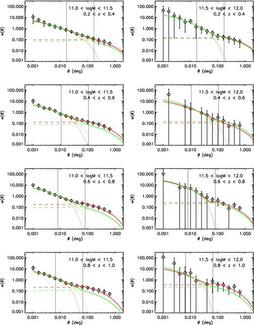
The measured angular correlation functions (diamonds) for the 10^11.0−11.5 M_⊙ (left panels) and the 10^11.5−12.0 M_⊙ (right panels) galaxies at z = 0.2–0.4, 0.4–0.6, 0.6–0.8 and 0.8–1.0, from top to bottom. The error bars represent the 2σ uncertainties of the measurements. The green and red curves show the best-fitting HOD models of the cases (i) and (ii), respectively (see text); the dotted and dashed lines represent the one-halo and two-halo terms, respectively, and the solid lines represent their sums. The thin vertical lines mark the comoving scales of 0.5 and 5 h⁻¹ Mpc at each redshift.

Open in new tabDownload slide

Figure 2

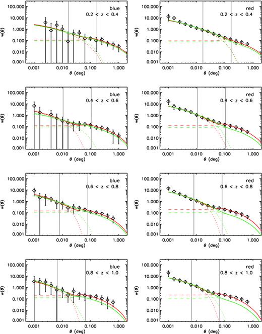
Same as Fig. 1, but for the blue (left panels) and the red (right panels) galaxy populations.

Open in new tabDownload slide

3 HALO OCCUPATION DISTRIBUTION MODELS

We investigate the evolutionary link of the observed galaxies to underlying dark (CDM) haloes by using HOD (see Cooray & Sheth 2002, for a review) models. HOD modelling is a powerful approach to explore galaxy distribution within dark haloes,whose formation and evolution can be predicted by simulations and analytic methods. Observations can provide the useful insights into underlying dark haloes by constraining HOD parameters in such a way that the models appropriately reproduce measured clustering properties of galaxies (e.g. Zehavi et al. 2005; Lee et al. 2006). In this work we follow Blake, Collister & Lahav (2008) for constructing our HOD models (see also Tinker et al. 2005). We give a short description of the models below, while the reader is referred to the above papers and the references therein for further details.

3.1 Model construction

In the HOD models we use the halo mass function n(M) presented by Jenkins et al. (2001). We assume the scale-dependent bias following Tinker et al. (2005), with the bias function b(M) taken from the Sheth, Mo & Tormen (2001) model including the revised parameters given by Tinker et al. (2005). The non-linear dark-matter power spectrum is constructed using the fitting formulae of Smith et al. (2003). The dark halo density profile of Navarro, Frenk & White (1997) is adopted, with the characterizing concentration parameter c(M) calibrated by numerical simulations (Bullock et al. 2001).

The statistical number of a central galaxy within a dark halo of the mass M is parametrized as

4

where erf (x) is the error function (Zheng et al. 2005). The haloes above a threshold mass of M_cut have a single central galaxy and those below M_cut have no central galaxies on average, while the transition between the two cases is softened by the parameter σ_cut. We adopt σ_cut = 0.3, which is the mean value found for luminous red galaxies at z < 1 (Blake et al. 2008; Brown et al. 2008). The number of satellite galaxies is described as the power-law form

5

The total number of galaxies populating a dark halo is given by

6

thus no galaxies are statistically found in the dark haloes below the threshold mass M_cut. We show an example of our HOD model along with the adopted halo mass function in Fig. 3.

Figure 3

An example of the HOD model N(M) and the halo mass function n(M). The HOD model is calculated with the parameter values M_cut = 10¹³ M_⊙, M₀ = 10¹⁴ M_⊙ and β = 1.5. The dotted lines represent the numbers of central galaxies N_cen(M) and satellite galaxies N_sat(M), and the solid lines represent the total number N(M) =N_cen(M) [1 +N_sat(M)]. The dashed lines show the evolving halo mass function at z = 0.3, 0.5, 0.7 and 0.9, from top to bottom. An actual number of galaxies hosted in a halo with the mass M in a given volume scales as n (M) ×N(M).

Open in new tabDownload slide

A spatial clustering of galaxies ξ (r) can be divided into the two terms, namely, a one-halo term [ξ_1h(r)] arising from pairs of galaxies in the same dark halo, and a two-halo term [ξ_2h(r)] arising from pairs of galaxies that reside in different haloes:

7

The one-halo term dominates a correlation function at small scales ≲ a few h⁻¹ Mpc, i.e. less than a typical virial diameter of large haloes, while a two-halo term becomes dominant at larger scales. The halo exclusion (which implements the condition that haloes cannot reside within each other) is considered by introducing the truncation mass, above which the haloes would overlap with each other at the separation r, into the calculation of ξ_2h(r). The truncation mass is derived using the ‘n′_g-matched’ approximation described in Tinker et al. (2005). The spatial correlation ξ (r) is projected to the angular correlation function w (θ) via

8

where x (z) is the comoving radial distance to the redshift z. The redshift distribution of galaxies, p (z), is estimated by giving the random gaussian errors with the standard deviation σ_Δz/(1+z)∼ 0.04, which corresponds to our photometric-redshift uncertainty, to the interpolated number-density evolution reported in Matsuoka & Kawara (2010) (including the local measurements by Cole et al. 2001) multiplied by the comoving volume element, and then extracting the true redshift distribution of the sources found in the disturbed-redshift bin under consideration. However, we find that the resultant HOD parameters presented below are not very sensitive to the details of the p(z) function. We show the examples of the calculated ACFs with the several sets of the HOD parameters in Fig. 4.

Figure 4

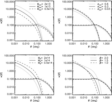
The dependence of the predicted ACF on the HOD parameters. In each panel the two curves of the same line style represent the one-halo and the two-halo terms, the former being dominant at small angular scales. The basic parameters are (M_cut, σ_cut, M₀, β) = (10¹³ M_⊙, 0.3, 10¹⁴ M_⊙, 1.5) and one of the parameter values is altered in each panel as indicated at the top right corner. Note that σ_cut is fixed to 0.3 in the present work.

Open in new tabDownload slide

From the above parametrization of the HOD N (M) along with the halo mass function n(M) and the bias function b (M), we can calculate some useful quantities; the number density of galaxies:

9

the effective large-scale bias:

10

the effective mass of the host dark halo:

11

and the average fraction of central or satellite galaxies:

12

3.2 Other models

Note that the above HOD form is based on a theoretical galaxy sample above a certain baryonic mass threshold, predicted by smoothed particle hydrodynamics (SPH) simulations and semi-analytic galaxy formation models (Berlind et al. 2003; Zheng et al. 2005). While our galaxy sample is defined by the stellar-mass bins rather than thresholds, we use the above models in this work for the following reasons. First, our massive galaxies are located at the steep high-end part of the mass function, so that the galaxies above the upper limit of a stellar-mass bin have little impact on the observables whether they are included in the measurements or not. In fact we find no significant difference in the measured number densities and ACFs between the M_★ = 10^11.0−11.5 M_⊙ and M_★ > 10^11.0 M_⊙ galaxy samples or between the M_★ = 10^11.5−12.0 M_⊙ and M_★ > 10^11.5 M_⊙ galaxy samples. Second, we actually find that adding an upper cut-off to N_cen(M) does not provide the better fits to the observed ACFs than the standard model does, while it is proposed to reproduce the HOD of galaxies in stellar-mass bins (see below). Third, the adopted model can approximate the HODs of various kinds of galaxies with a minimum number of parameters (Zheng et al. 2005), which is essential in exploring the halo characteristics of galaxies with relatively large errors in the ACF measurements, such as our sample.

We have examined the effects of changing HOD models as follows. The standard model is modified by considering the variable σ_cut, fixed β and/or the additional cut-off parameter M₁ of the satellite HOD:

13

We have also tried the six-parameter form:

14

which is constructed to reproduce the HODs of a sample of galaxies in a stellar-mass bin or of young (in terms of stellar age) galaxies presented by Zheng et al. (2005). The essential difference of this form from our standard one is that it allows an upper cut-off of N_cen(M). In addition, we have replaced the whole model construction process (from the choice of dark-matter power spectrum) from the above one following Blake et al. (2008) to the one following the recipe given by Hamana et al. (2004), who adopt the HOD form of

15

We have also tried a few other halo mass functions (Sheth & Tormen 1999; Reed et al. 2007; Bhattacharya et al. 2010) and bias functions (Sheth & Tormen 1999; Tinker et al. 2010a). However, we find that none of the above altered models provides a better reproduction of the observed ACFs than our standard model does.

3.3 Results

We constrain the parameters M_cut, M₀ and β of the standard HOD model by comparing the predicted ACFs [w^th(θ)] and number densities (n^th_gal) with those observed [w^obs(θ) and n^obs_gal] through the Markov chain Monte Carlo (MCMC) method. The observed number densities are taken from Matsuoka & Kawara (2010). We evaluate the likelihood of the specific model by the χ² value of the model fit to the observed quantities. The ACF fitting is restricted to the angular scales θ < 0.3 deg where the effects of the integral constraint (i.e. the boundary effect of the observations) are negligible.

We summarize the obtained best-fitting HOD parameters in Table 2 (the former values in the parentheses). In the case of the 10^11.5−12.0 M_⊙ galaxies at 0.6 < z < 0.8, the parameter β is not well constrained in the plausible range (β < 3) and we fix it to the best-fitting value found for the 10^11.0−11.5 M_⊙ galaxies at the same redshift range (it is justified by the fact that we find the consistent β values for the two populations at other redshifts). The poor constraint on β is caused by the fact that the three HOD parameters correlate with each other in reproducing a given ACF, hence the MCMC fitting could converge to unrealistic combinations of the parameter values when a measured ACF is accompanied by large uncertainty. In other subsamples, plausible values of β are obtained; we find β = 1.5 –2.0 for all but the blue subsamples, which are in good agreement with those found for SDSS luminous red galaxies at 0.4 < z < 0.7 measured by Blake et al. (2008).

The ACFs of the best-fitting HOD models are overlaid on the observed ACFs in Figs 1 and 2 (green curves). In these fittings, the systematic discrepancy between the model and measured ACFs are observed at the large angular scales where two-halo terms dominate the ACFs. The reason for this discrepancy is fairly clear; the observed ACFs are so strong that very massive haloes are required to reproduce them, while the predicted number of such massive haloes is very small compared to the observed numbers of massive galaxies (the further discussion is given below). As a reference, we have carried out another set of model fittings with the modified requirement that the models should only reproduce the observed ACFs, imposing no constraint on the predicted number densities of galaxies. We refer to this second set of model fittings as case (ii), and the original fittings as case (i) hereafter. The results of the former case are listed in Table 2 (the latter values in the parentheses) and are shown in Figs 1 and 2 by the red curves. We obtain the excellent fits of the ACFs in the case (ii) over the entire angular scales, while the predicted n^th_gal are smaller than n^obs_gal in the most cases.

4 DISCUSSION

As a starting point for the discussion, we show the amplitudes of the measured ACFs at the comoving scales of 0.5 and 5 h⁻¹ Mpc in Fig. 5. They are derived by interpolating the data points in Figs 1 and 2 with the best-fitting HOD models of the case (ii).1 The two comoving scales are chosen to represent the clustering within a halo (i.e. one-halo term) or between haloes (i.e. two-halo term), considering the typical diameter of a few h⁻¹ Mpc for large haloes. Apparently the ACF amplitudes are larger in more massive or redder galaxies at both scales. In other words, we find that more mature (hence massive or red) galaxy systems are more clustered. It is the expected result if the more mature galaxies have started stellar-mass assembly earlier within the highly biased region where the structure formation has also started earlier. The larger diversity of the ACF amplitudes at 0.5 h⁻¹ Mpc than at 5 h⁻¹ Mpc reflects the fact that the one-halo term is much more dependent on the HOD details of each galaxy population than the two-halo term is. The two-halo term is mainly determined by the spatial distribution of host haloes rather than those of galaxies within a halo, hence its dependence on the HOD parameters is much weaker than that of the one-halo term. This is clearly seen in Fig. 4.

Figure 5

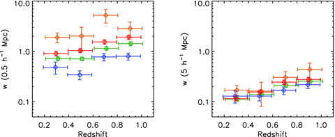
The ACF amplitudes at the comoving scales of 0.5 h⁻¹ Mpc (left) and 5 h⁻¹ Mpc (right) measured for the 10^11.0−11.5 M_⊙ (green), the 10^11.5−12.0 M_⊙ (orange), the blue (blue) and the red (red) galaxies. The data points are slightly shifted along the redshift axis relative to each other for visibility.

Open in new tabDownload slide

In the HOD model fitting, we consider the two cases with the different requirements for the models. They are defined in Section 3.3 and are summarized in Table 3. As already noted, the observed ACFs are so strong that very massive haloes are required to reproduce them, while such massive haloes are extremely rare and could not host the observed number of massive galaxies. While a small number of haloes could host a large number of massive galaxies if the majority of the galaxies are satellites, such an HOD results in very strong ACF amplitudes at small scales, which conflicts with the present measurements (hence is not selected in the above fittings). The case (i) models provide a comparable number of galaxies to the observed by including the host haloes whose masses are presumably lower than in reality, hence the predicted ACFs are weaker than the observed. Therefore, the derived halo masses and biases in the case (i) should be regarded as the lower limits. Case (ii) takes the opposite approach by selecting only the most massive haloes in order to reproduce the observed strong ACFs, while setting aside the majority of the observed galaxies presumably hosted by lower-mass haloes. Thus the derived halo masses and biases should be the strict upper limits. We will discuss this issue further below. The actual HOD parameter values of the galaxies should be somewhere in between those of the above two extreme cases, and we conservatively adopt the above upper and lower limits in this work.

In Fig. 6 we show the derived bias factors and halo mass estimates as a function of redshift. It is clearly seen that the most massive galaxies mark the most biased density structure of dark matter distributions, as expected. The threshold mass for hosting a central galaxy, M_cut, is significantly larger for more massive galaxies, which is consistent with the general agreement that the capability of hosting massive galaxies depends strongly on halo mass. The typical mass for hosting a satellite galaxy, M₀, is extremely large (∼10¹⁴⁻¹⁶ M_⊙), which means that only the most massive haloes could host a galaxy with the stellar mass exceeding 10¹¹ M_⊙ as a satellite. Actually we find that the fractions of central galaxies f_cen in the current sample are larger than 90 per cent in most cases. These results are the consequence of the relative weakness of the observed ACFs at small scales (one-halo terms, arising from central–satellite pairs) compared to those at large scales (two-halo terms, mainly arising from central–central pairs in the current case). While the effective halo mass M_eff shows a similar trend to M_cut with regard to the galaxy stellar mass, the difference of the M_eff between the 10^11.0−11.5 M_⊙ and the 10^11.5−12.0 M_⊙ galaxies are less than those of the M_cut. It is because of the negative and steepening slope of the halo mass function toward high-mass end; increasing M_cut is accompanied by the smaller increment of M_eff since there are less and less haloes as the halo mass increases. The stellar-mass to halo-mass ratios are found to be M_★/M_eff∼ 0.003. We observe no significant difference of the ratios between the different stellar-mass classes, while the ratios might be very marginally larger for more massive systems, which indicates that the fractional mass growth rate (⁠⁠) of haloes are comparable to or marginally lower than those of stellar systems above M_★∼ 10¹¹ M_⊙ (i.e. ⁠). The major mass accretion would have already terminated for these very massive haloes, while the stellar-mass assembly of the massive galaxies would also be inefficient since they are located near the high-mass end of the galaxy mass function.

Figure 6

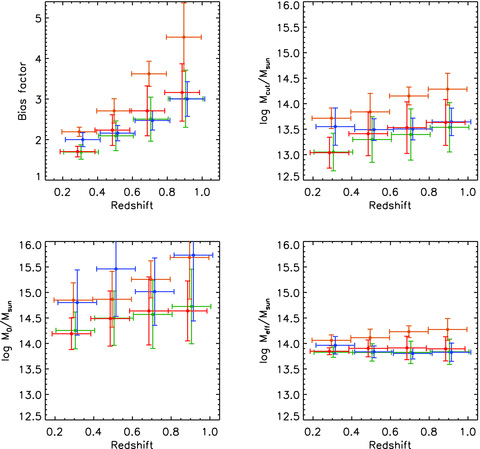
Halo occupation distribution of massive galaxies as a function of redshift (top left: b_gal, the bias factor; top right: M_cut, the threshold mass for hosting a central galaxy; bottom left: M₀, the typical mass for hosting a satellite galaxy; bottom right: M_eff, the effective mass of host haloes). The green, orange, blue and red bars represent the 10^11.0−11.5 M_⊙, the 10^11.5−12.0 M_⊙, the blue and the red galaxies, respectively.

Open in new tabDownload slide

We note that the derived effective masses of haloes, M_eff∼ 10¹⁴ M_⊙, are comparable to the halo masses found for galaxy clusters (e.g. Lin & Mohr 2004; Lin, Mohr & Stanford 2004). Considering the high fraction of central galaxies (f_cen > rsim 0.9), the massive galaxies studied here are presumably equivalent to central galaxies of galaxy clusters. Actually, the stellar masses of M_★ > 10¹¹ M_⊙ are typical of the central galaxies of galaxy groups or clusters with the halo masses ∼10¹⁴ M_⊙ (Yang, Mo & van den Bosch 2008), which is comparable to the current estimates of the effective halo mass.

Fig. 6 shows that the bias factor clearly decreases with decreasing redshift. It implies rapid evolution of dark matter distributions while the clustering structures traced by the massive galaxies evolve relatively slowly. The halo mass M_cut also shows a marginal decline toward the local Universe, which might suggest that the M_★ > 10¹¹ M_⊙ galaxies are formed in progressively less massive haloes with cosmic time. Then it might imply that the fractional mass growth rate of stellar systems exceeds those of haloes (⁠⁠) for the relatively low-mass (M_★ < 10¹¹ M_⊙) galaxies, a part of which eventually evolve into the massive galaxies.

We observe no clear difference of the HODs between the blue and the red galaxies in Fig. 6. It contrasts with the measured ACF amplitudes plotted in Fig. 5, where the red galaxies clearly show higher degree of clustering than the blue galaxies. The difference between the two populations disappears in the derived HODs due to the relative scarcity of the massive blue galaxies; since the current HOD models predict that both populations are mostly central galaxies and assume that the probability of hosting a central galaxy is a monotonically increasing function of halo mass, the numerous red central galaxies require relatively low-mass haloes as their hosts compared to the scarce blue galaxies. Thus the derived halo masses (and biases) of the red galaxies become relatively low, which cancels out the higher ACF amplitudes measured for the red galaxies [indeed the larger halo masses or biases are predicted for the redder galaxies in the case (ii) which imposes no constraints on the predicted galaxy number density].

However, the HOD assumption that the probability of hosting galaxies is a monotonically increasing function of halo mass could be too simplistic, particularly for massive blue galaxies. It is possible that galaxies in massive, grown-up haloes have exhausted most of their gas and have systematically lower level of star formation. In addition, recent studies suggest star-formation quenching mechanisms of massive galaxies as a feedback process of galaxy mass assembly, such as the onset of active galactic nuclei (e.g. Silk & Rees 1998; Granato et al. 2004; Springel, Di Matteo & Hernquist 2005). These processes could systematically reduce the number of massive blue galaxies in massive haloes, in a way dependent on halo characteristics and galaxy star-formation and its quenching physics. We also note that fitting the ACFs of the blue and red galaxies separately with the current HOD models might be problematic, since the haloes hosting a red central and blue satellites, or a blue central and red satellites, cannot be properly reproduced. These situations might be mimicked by the HOD forms such as those given by the equation (14), which allows an upper cut-off in N_cen and reproduces the HODs of ‘young’ galaxies presented by Zheng et al. (2005), but we do not obtain improved fits of the ACFs with this form as compared to those with our standard model. However, since the HODs of the massive blue galaxies could be significantly altered by considering the more numerous red populations, the central fractions of massive blue galaxies deduced above are rather tentative. Further investigation of this issue is beyond the scope of this paper, and would require much more precise clustering measurements of massive blue galaxies. If the observed scarcity of the massive blue galaxies is due to the star-formation quenching physics rather than their need for very massive host haloes, then one might be able to conclude, simply from Fig. 5, that massive blue galaxies reside in less massive haloes than the hosts of massive red galaxies. Again, it would be the natural result if redder galaxies have started stellar-mass assembly earlier within the region where the halo mass assembly has also started earlier.

Finally, we comment on the discrepancy between the HOD model predictions and the observed quantities. As stated above, the observed ACFs are so strong that very massive haloes are required to reproduce them, while such massive haloes are extremely rare and could not host the observed number of massive galaxies. It is unlikely that most of the massive galaxies are hosted by a small number of such massive haloes as satellites, since it would result in much stronger ACFs than observed at small angular scales. The discrepancy between the observed and model ACFs in the case (i) tends to increase with increasing redshift (see Figs 1 and 2). In this regard, we note that a similar discrepancy is observed in the analysis of distant red galaxies at z∼ 2.3 by Tinker, Wechsler & Zheng (2010b) (see also Quadri et al. 2008). The systematic difference between their model and observed ACFs at large angular scales is roughly a factor of 2 (while within the 1σ uncertainty of their measurements), which is comparable to those found in our sample. As raised by Quadri et al. (2008), the underlying cause of the problem might be that the current HOD models are too simplistic. While the current models assume that a number of galaxies hosted in a halo depends solely on the halo mass, other halo characteristics such as the mass accretion rate could affect the galaxy formation and alter the observed properties of galaxies within the halo. We also note that fitting the clusterings of different galaxy populations (e.g. blue and red galaxies) at the same time may improve the situation, while such an analysis would significantly increase the number of HOD parameters and require much precise data for clustering measurements. Furthermore, we can raise the possibility that the evolution of halo mass function and/or bias function is not well understood; our results might point to the earlier emergence of massive haloes (i.e. larger numbers of massive haloes at high redshifts) than predicted in the current halo models.

It is also worth pointing out that the observed ACFs are apparently larger than the fitted HOD models at the smallest angular scales (θ∼ 0.001 deg). These close pairs may represent interacting galaxies (e.g. Roche et al. 1999). Reproducing such a feature by the HOD models requires the detailed description of galaxy interaction within a halo. However, our focus here is the global characteristic of the host haloes and such an investigation is a subject of future papers.

5 SUMMARY

In this work we present a clustering analysis of ∼60 000 massive (stellar mass M_★ > 10¹¹ M_⊙) galaxies taken from Matsuoka & Kawara (2010). The galaxies have been extracted from 55.2 deg² of the UKIRT Infrared Deep Sky Survey (UKIDSS) and the Sloan Digital Sky Survey (SDSS) II Supernova Survey, and are nearly complete to z = 1 with robust estimates of photometric redshift and stellar mass. We classify them based on stellar masses (M_★ = 10^11.0−11.5 M_⊙ or 10^11.5−12.0 M_⊙) and rest-frame colours (blue: U−V < 1.0, red: U−V > 1.0), in order to reveal the difference in the spatial distributions of different galaxy populations.

The ACFs of the galaxies are quantified using the Landy & Szalay (1993) estimator, and we find strong clustering detected for all the subsamples. In order to interpret the measured ACFs, we construct HOD models following Blake et al. (2008) and compare the predicted ACFs with the observed. Our major findings are as follows.

• The clustering amplitudes clearly show a systematic trend regardless of the measured redshift, in which the most massive, 10^11.5−12.0 M_⊙ galaxies have the strongest clustering and the blue galaxies have the weakest clustering. It would be the natural result if more mature galaxies have started stellar-mass assembly earlier within the highly biased region where the halo-mass assembly has also started earlier.

• The bias factors and halo masses are systematically larger for the galaxies with larger stellar masses, which confirms that the capability of hosting massive galaxies depends strongly on halo mass. The stellar-mass to halo-mass ratios are M_★/M_eff∼ 0.003, with no significant difference observed between the different stellar-mass classes.

• The inferred halo masses of M_eff∼ 10¹⁴ M_⊙ and the high central fractions (f_cen > rsim 0.9) indicate that the massive galaxies in the current sample are equivalent to central galaxies of galaxy clusters.

• The bias factor decreases with decreasing redshift, which implies rapid evolution of dark matter distributions while the clustering structures traced by the massive galaxies evolve relatively slowly. The halo mass M_cut also shows a marginal decline toward the local Universe, which might suggest that massive (M_★ > 10¹¹ M_⊙) galaxies are formed in progressively less massive haloes with the cosmic time.

• If the observed scarcity of massive blue galaxies is due to the star-formation quenching physics rather than their need for very massive host haloes, then one might be able to conclude that massive blue galaxies reside in less massive haloes than the hosts of massive red galaxies.

• The observed ACFs are so strong at large angular scales that very massive haloes are required to reproduce them, while such massive haloes are extremely rare and could not host the observed number of massive galaxies. It might point to the inadequacy of the current HOD models or a lack of knowledge about the evolving halo mass function and/or bias function.

We are grateful to K. Shimasaku, K. Kohno, J. Makino, N. Yasuda, and N. Yoshida for insightful discussions and suggestions. We thank the referee for his/her useful comments which helped to improve this paper. YM acknowledges Grant-in-Aid from the Research Fellowships of the Japan Society for the Promotion of Science (JSPS) for Young Scientists. This work was supported by Grants-in-Aid for Scientific Research (17104002, 21840027, 22684005), Specially Promoted Research (20001003), Specially Promoted Research on Inovated Area (22111503), and the Global COE Program of Nagoya University ‘Quest for Fundamental Principles in the Universe (QFPU)’ from JSPS and MEXT of Japan.

REFERENCES