The γ-ray brightest days of the blazar 3C 454.3 Free

Abstract

1 INTRODUCTION

Among the flat-spectrum radio quasar (FSRQ) class of blazars, 3C 454.3 (z = 0.859; Jackson & Browne 1991) is one of the brightest and most variable sources. In 2005 April–May, it underwent a dramatic optical outburst, reaching its historical maximum with R = 12.0 (Villata et al. 2006). This exceptional event triggered observations at X-ray energies with the INTEGRAL (Pian et al. 2006) and the Swift satellites (Giommi et al. 2006). These detected the source up to 200 keV and in a brightened hard X-ray state. This strong optical and hard X-ray activity was followed by a radio outburst with about 1-yr delay (Villata et al. 2007). Despite this extraordinary activity, the lack of a γ-ray satellite at that time prevented us from concluding that this activity was due to a real increase of the jet power, since the integrated optical luminosity was of the same order of the γ-ray luminosity observed, years before, by the EGRET instrument on-board the Compton Gamma-Ray Observatory (CGRO) satellite (Nandikotkur et al. 2007). After the launch of AGILE, 3C 454.3 was seen to be very bright (Vercellone et al. 2007) and variable in the γ-ray band, being often the brightest γ-ray blazar in the sky (Vercellone et al. 2010), even if the simultaneous optical states were much fainter than during the 2005 flare. Many other active phases followed also in 2008 summer just after the launch of the Fermi satellite (Tosti et al. 2008; Abdo et al. 2009a), and in 2009 summer–fall, when the source was detected in active state all across the entire electromagnetic spectrum leading to many Astronomer's Telegrams (ATels) (Bonning et al. 2009; Buxton et al. 2009; Gurwell 2009; Hill 2009; Striani et al. 2009a; Villata et al. 2009). This activity climaxed in 2009 December, when an extraordinary γ-ray flare occurred on December 2, seen by AGILE (Striani et al. 2009b), Fermi/Large Area Telescope (LAT) (Escande & Tanaka 2009), Swift/X-ray Telescope (XRT) (Sakamoto et al. 2009) and Swift/Burst Alert Telescope (BAT) (Krimm et al. 2009).

In the case of the 2007 flare, it was possible to model its spectral energy distribution (SED) in different states with a jet whose total power was nearly constant in time (Katarzynski & Ghisellini 2007), but whose dissipation region was located at different distances R_diss from the central power house (Ghisellini et al. 2007). In this model, the magnetic field energy density scales as U_B∝ (ΓR_diss)⁻², where Γ is the bulk Lorentz factor. Conversely, the radiation energy density U_ext produced by the broad-line clouds scales as Γ² and is independent of R_diss as long as the dissipation region is within the broad-line region (BLR). Even if the latter is most likely stratified, the contribution of the Lyα line to the BLR luminosity is dominant, and we identify the size of the BLR with the shell mostly emitting the Lyα photons. As a consequence, U_B/U_ext∼L_opt/L_γ∝R⁻²_dissΓ⁻⁴. Even with a constant and dominating L_γ and a constant Γ, we can have large variations of the optical flux by changing R_diss. These ideas were borne out in Ghisellini et al. (2007), immediately after the AGILE detection of a very bright γ-ray state accompanied by a moderate optical flux; the optical synchrotron flux can vary by a large amount even if the jet continues to carry the same power and always dissipates the same fraction of it. This assumes and implies, however, that the bulk of the electromagnetic output is in the more energetic inverse Compton component, that in this case should remain quasi-steady.

Instead, the large outburst seen in 2009 December witnessed a dramatic increase of this component. In this case, it is very likely that the power dissipated by the jet indeed increased, and it is likely that this is the consequence of an increase of total power carried by the jet. The luminosity reached in γ-rays exceeded L_γ∼ 3 × 10⁴⁹ erg s⁻¹, a factor of ∼30 larger than the EGRET luminosity, and also larger than the 2007 AGILE state. The goal of our present study is first to characterize the emission properties of 3C 454.3 during the 2009 November–December period, then to find the physical properties of the jet during the flare and finally to compare those with the luminosity of the accretion disc. In fact, as we shall see, the power of the jet of 3C 454.3 in the first week of 2009 December likely surpassed the luminosity of the accretion disc.

We use H₀ = 70 km s⁻¹ Mpc⁻¹ and Ω_M = 0.3, Ω_Λ = 0.7 and use the notation Q = 10^xQ_x in cgs units.

2 DATA & ANALYSIS

2.1 Data sets

This study is focused on the analysis of the multiwavelength (MWL) data gathered by the Fermi and Swift satellites in the period between 2009 November 1 and December 14. From these data we obtained day-scale resolved light curves along the whole time-span, in the γ-ray, X-ray and optical–UV band. Moreover, for some selected days we derived the spectral information needed to study the simultaneous MWL SED. These data sets are labelled according to the observation date.

In order to fully characterize the evolution of the SED across the whole dynamic range of γ-ray flux observed by Fermi, we also built a ‘low’ SED, deriving an HE spectrum of 3C 454.3 from an earlier period of observation when the source was significantly weaker in γ-rays, and matching it with Swift data from the same period.

Finally, in order to better investigate the UV portion of the SED, we matched an archival UV spectrum of 3C 454.3 observed by the Galaxy Evolution Explorer (GALEX) satellite with contemporary optical–UV data taken by Swift.

2.2 Fermi/LAT

We retrieved from the NASA data base1 the publicly available data from the LAT γ-ray telescope on-board of the Fermi satellite (Atwood et al. 2009). We selected the good quality (‘DIFFUSE’ class) events observed within 10° from the source position (J2000) ⁠, but excluding those observed with zenith distance of the arrival direction greater than 105°, in order to avoid contamination from the Earth albedo. We performed the analysis by means of the standard science tools, v. 9.15.2, including Galactic and isotropic extragalactic backgrounds and the P6 V3 DIFFUSE instrumental response function. For each data set (and, in case of spectra, for each energy bin), we calculated the lifetime, exposure map and diffuse response of the instrument. Then we applied to the data an unbinned likelihood algorithm (gtlike), modelling the source spectrum with a power-law model, with the integral flux in the considered energy band and photon index left as free parameters. The minimum statistical confidence level (CL) accepted for each time (or time and energy, in the case of spectra) bin is TS = 10, where TS is the test statistic described in Mattox et al. (1996, see also Abdo et al. 2009b). Quoted errors are statistical, at 1σ level. Systematic flux uncertainties are within 10 per cent at 100 MeV, 5 per cent at 500 MeV and 20 per cent at 10 GeV (Rando 2009).

2.2.1 Light curve

In the upper panel of Fig. 1, we report the integral γ-ray flux above 100 MeV, calculated in 1-d time bins for the period from 2009 November 1 to December 14. The flux level is always above 10⁻⁶ cm⁻² s⁻¹, the clear signature of a coherent γ-ray active phase. On December 2, the flux reached the extreme value of (21.8 ± 1.2) × 10⁻⁶ cm⁻² s⁻¹, the strongest non-gamma-ray burst flux measured by a γ-ray satellite. The corresponding observed γ-ray luminosity is of the same order of PKS 1502+106 in outburst (Abdo et al. 2010a).

Figure 1

Light curve above 100 MeV (top), in the (0.2–10 keV) X-ray band (middle panel) and in the different UVOT filters (bottom panel, as labelled). Note the logarithmic y-axes, and their different scales. Yellow lines mark the days for which simultaneous MWL SED were derived and modelled.

Open in new tabDownload slide

2.2.2 Spectra

The exceptional flux level of 3C 454.3 in late 2009 allowed for the first time to derive day-scale γ-ray spectra with good quality; usually an inconceivable task for space-based instruments due both to their small collection area and the weak flux of the HE sources. This opens new opportunities for the study of the MWL SED of this FSRQ on short time-scales, hopefully allowing deeper insight into the engine and the emission mechanism.

In this study, we use LAT spectra produced with data from only a few single days, selected within the period covered also by Swift observations. We have chosen to construct the SEDs in order to cover the whole flux range of the campaign. We therefore selected November 6, showing the lowest Ultraviolet–Optical Telescope (UVOT) fluxes of the whole period; November 27, a day in the rising phase of the flare, with intermediate γ-ray flux and the three days (December 1, 2 and 3) around the peak, in order to better investigate the evolution of the SED around this extreme phase. For the γ-ray spectrum of November 6, we decided to add the data from the following day (November 7), as it showed compatible γ-ray flux level, to improve the signal-to-noise ratio of the spectrum. Finally, we selected from the 18-months daily light curve (see e.g. Tavecchio et al. 2010) a longer time-span (15 Ms), starting from 2008 December 3 to 2009 May 26, when the source was at the lowest flux levels (F_{>100 MeV}∼ 5 × 10⁻⁷ cm⁻² s⁻¹) since the beginning of LAT observations. The derived HE spectrum allowed to explore the whole available dynamic range of 3C 454.3 γ-ray emission. For each data set, we split the LAT observed band in logarithmically spaced energy bins, and applied in each the unbinned likelihood algorithm. In addition to the request that TS > 10, we further requested that the model predicted at least five photons from the source; when needed, we merge in a single, wider bin the HE bins that did not fulfil this last request. These quality criteria are similar (and somehow more restrictive) to those adopted by Abdo et al. (2010b). For each spectrum, we cross-checked this analysis performed in bins of energy with an unbinned analysis on the whole 0.1–100 GeV band, where we modelled the source with a broken power-law model, in agreement with Abdo et al. (2010b). The results of the two methods were consistent within errors, even if the analysis in bins of energy, that does not exploit the full information of the event distribution across the whole LAT bandpass, leads to wider error bars. We report in Table 1 the parameters of the model, while the SED points are plotted in Fig. 4.

Table 1

Open in new tab

Results of the γ-ray analysis on Fermi-LAT data; only the data set used for the MWL SED are reported. For each data set, the effective source on-time t_on, the photon indices Γ₁ and Γ₂, the break energy E_break, the integral flux in the 0.1–100 GeV band F_{0.1-100 GeV} and the TS value of the unbinned likelihood analysis are reported. Uncertainties are statistical only, at 1σ level; systematics on flux measurement are within 10 per cent at 100 MeV, within 5 per cent at 500 MeV and within 20 per cent at 10 GeV. For the 06/11/09 data set, the relative weakness of the flux makes perfectly adequate a simple power-law model which is also reported for reference.

Obs. date dd/mm/yy	ton (ks)	Γ1	Γ2	Ebreak (GeV)	F0.1-100 GeV (10−6 ph cm−2 s−1)
Low	5.9 × 103	2.33 ± 0.03	3.37 ± 0.27	2.00 ± 0.38	0.61 ± 0.02	4687
06/11/09	61	2.66 ± 0.21	3.80 ± 1.20	1.10 ± 0.57	2.10 ± 0.30	218
		2.78 ± 0.16	–	–	2.15 ± 0.30	218
27/11/09	37	2.13 ± 0.10	3.17 ± 0.54	1.94 ± 0.56	7.58 ± 0.68	900
01/12/09	44	2.33 ± 0.11	3.15 ± 0.38	0.97 ± 0.34	10.76 ± 0.87	1100
02/12/09	39	2.37 ± 0.06	3.17 ± 0.46	2.70 ± 0.26	21.6 ± 1.2	2497
03/12/09	40	2.28 ± 0.06	3.42 ± 0.87	5.86 ± 0.36	15.94 ± 0.98	1915

Obs. date dd/mm/yy	ton (ks)	Γ1	Γ2	Ebreak (GeV)	F0.1-100 GeV (10−6 ph cm−2 s−1)
Low	5.9 × 103	2.33 ± 0.03	3.37 ± 0.27	2.00 ± 0.38	0.61 ± 0.02	4687
06/11/09	61	2.66 ± 0.21	3.80 ± 1.20	1.10 ± 0.57	2.10 ± 0.30	218
		2.78 ± 0.16	–	–	2.15 ± 0.30	218
27/11/09	37	2.13 ± 0.10	3.17 ± 0.54	1.94 ± 0.56	7.58 ± 0.68	900
01/12/09	44	2.33 ± 0.11	3.15 ± 0.38	0.97 ± 0.34	10.76 ± 0.87	1100
02/12/09	39	2.37 ± 0.06	3.17 ± 0.46	2.70 ± 0.26	21.6 ± 1.2	2497
03/12/09	40	2.28 ± 0.06	3.42 ± 0.87	5.86 ± 0.36	15.94 ± 0.98	1915

Table 1

Open in new tab

Results of the γ-ray analysis on Fermi-LAT data; only the data set used for the MWL SED are reported. For each data set, the effective source on-time t_on, the photon indices Γ₁ and Γ₂, the break energy E_break, the integral flux in the 0.1–100 GeV band F_{0.1-100 GeV} and the TS value of the unbinned likelihood analysis are reported. Uncertainties are statistical only, at 1σ level; systematics on flux measurement are within 10 per cent at 100 MeV, within 5 per cent at 500 MeV and within 20 per cent at 10 GeV. For the 06/11/09 data set, the relative weakness of the flux makes perfectly adequate a simple power-law model which is also reported for reference.

Obs. date dd/mm/yy	ton (ks)	Γ1	Γ2	Ebreak (GeV)	F0.1-100 GeV (10−6 ph cm−2 s−1)
Low	5.9 × 103	2.33 ± 0.03	3.37 ± 0.27	2.00 ± 0.38	0.61 ± 0.02	4687
06/11/09	61	2.66 ± 0.21	3.80 ± 1.20	1.10 ± 0.57	2.10 ± 0.30	218
		2.78 ± 0.16	–	–	2.15 ± 0.30	218
27/11/09	37	2.13 ± 0.10	3.17 ± 0.54	1.94 ± 0.56	7.58 ± 0.68	900
01/12/09	44	2.33 ± 0.11	3.15 ± 0.38	0.97 ± 0.34	10.76 ± 0.87	1100
02/12/09	39	2.37 ± 0.06	3.17 ± 0.46	2.70 ± 0.26	21.6 ± 1.2	2497
03/12/09	40	2.28 ± 0.06	3.42 ± 0.87	5.86 ± 0.36	15.94 ± 0.98	1915

Obs. date dd/mm/yy	ton (ks)	Γ1	Γ2	Ebreak (GeV)	F0.1-100 GeV (10−6 ph cm−2 s−1)
Low	5.9 × 103	2.33 ± 0.03	3.37 ± 0.27	2.00 ± 0.38	0.61 ± 0.02	4687
06/11/09	61	2.66 ± 0.21	3.80 ± 1.20	1.10 ± 0.57	2.10 ± 0.30	218
		2.78 ± 0.16	–	–	2.15 ± 0.30	218
27/11/09	37	2.13 ± 0.10	3.17 ± 0.54	1.94 ± 0.56	7.58 ± 0.68	900
01/12/09	44	2.33 ± 0.11	3.15 ± 0.38	0.97 ± 0.34	10.76 ± 0.87	1100
02/12/09	39	2.37 ± 0.06	3.17 ± 0.46	2.70 ± 0.26	21.6 ± 1.2	2497
03/12/09	40	2.28 ± 0.06	3.42 ± 0.87	5.86 ± 0.36	15.94 ± 0.98	1915

Figure 4

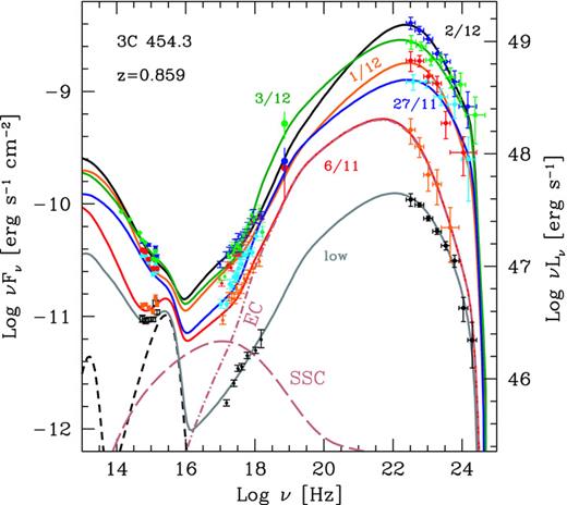
The SED of 3C 454.3 at six selected epochs: 2009 November 6 and 27; 2009 December 1, 2 and 3 plus the previous ‘low’γ-ray state (see text). The different SED are labelled. We also show the result of our modelling, including the accretion disc component, its X-ray corona contribution and the IR emission from the torus (dashed black lines). For the SED of November 6, we show also, for illustration, the contribution of the EC and SSC components. Note that both are necessary to explain the X-ray spectrum, according to our modelling.

Open in new tabDownload slide

2.3 Swift

We analysed the data from observations performed between 2009 November 1 and December 14. We also analysed data from late 2008 December, contemporary to the lowest γ-ray state of 3C 454.3 seen by Fermi. Finally, UVOT data from a pointing in 2008 October were analysed, as we wanted to compare this observation with a roughly simultaneous GALEX archival UV spectrum of the source (see Section 3.2).

The data from the two narrow-field instruments on-board Swift (Gehrels et al. 2004) have been processed and analysed with heasoft v. 6.8 and with the CALDB updated on 2009 December 30.

2.3.1 X-Ray Telescope

Data from the XRT (0.2–10 keV; Burrows et al. 2005) were analysed using the xrtpipeline task, set for the photon counting or window timing modes and having selected single pixel events (grade 0). In the case of the light curve, we converted the observed counts rates to fluxes assuming a common Γ=− 1.6 photon index and with absorption fixed at the Galactic value N^Gal_H = 6.6 × 10²⁰ cm⁻² derived from A_B = 0.46 (Raiteri et al. 2008). The resulting light curve is shown in the middle panel of Fig. 1.

We extracted the spectra in order to build SED simultaneous to Fermi/LAT by using default regions. Data were rebinned in order to have at least 30 counts per energy bin. Power-law models have been fitted to the spectra, except for two cases, the ‘low’ state and the spectrum from December 2, when a broken power-law model fitted the data significantly better (ftest >99 per cent). In Table 2 we report the spectral parameters for the observations used for modelling the SED.

Table 2

Open in new tab

Synopsis of the results of the X-ray analysis performed on Swift/XRT data. Only the data sets used for modelling the MWL SED of 3C 454.3 are reported. For each one of these, the exposure time t_exp, the photon indices Γ₁ and Γ₂, the break energy E_break, the normalization factor of the differential spectrum at 1 keV f₀, the observed (not de-absorbed) flux in the 0.2–10 keV band F_{0.2–10 keV}, the intrinsic luminosity in the same band L_{0.2–10 keV} and the goodness-of-fit statistic (reduced χ²) with the corresponding number of degrees of freedom (d.o.f.) are reported. The ‘low’ data set results from the addition of observations made between 2008 December 25 and 2009 January 01 (obsID from 00090023002 up to 00090023008) while the other data sets come from single pointings and are labelled with the date of observation. Spectra have been dereddened according to the N_H = 6.6 × 10²⁰ cm⁻² value derived from Raiteri et al. (2008). The errors on the observed fluxes are within the 10 per cent level (at 90 per cent CL).

Obs. date dd/mm/yy	ObsID	texp ks	Γ1	Γ2	Ebreak (keV)	f0 (10−2 ph cm−2 s−1 keV−1)	(10−11 erg cm−2 s−1)	L0.2−10 keV (1047 erg s−1)	(d.o.f.)
Low	See caption	9.0	1.13+0.30−0.24	1.13+0.30−0.24	1.40+1.00−0.36	0.15 ± 0.01	1.1	0.34	0.89 (43)
06/11/09	00035050070	1.0	1.52 ± 0.07	–	–	2.2 ± 0.2	6.6	2.1	0.96 (38)
27/11/09	00035050073	0.9	1.42 ± 0.06	–	–	3.0 ± 0.2	11.0	3.1	1.13 (53)
01/12/09	00035050074	1.1	1.43 ± 0.04	–	–	4.5 ± 0.3	16.0	4.5	1.08 (87)
02/12/09	00035050075	1.2	0.98+0.15−0.19	1.56 ± 0.07	1.2 ± 0.2	2.2 ± 0.2	17.0	4.8	0.98 (103)
03/12/09	00035050076	1.0	1.43 ± 0.04	–	–	5.2 ± 0.3	18.0	5.2	0.88 (89)

Obs. date dd/mm/yy	ObsID	texp ks	Γ1	Γ2	Ebreak (keV)	f0 (10−2 ph cm−2 s−1 keV−1)	(10−11 erg cm−2 s−1)	L0.2−10 keV (1047 erg s−1)	(d.o.f.)
Low	See caption	9.0	1.13+0.30−0.24	1.13+0.30−0.24	1.40+1.00−0.36	0.15 ± 0.01	1.1	0.34	0.89 (43)
06/11/09	00035050070	1.0	1.52 ± 0.07	–	–	2.2 ± 0.2	6.6	2.1	0.96 (38)
27/11/09	00035050073	0.9	1.42 ± 0.06	–	–	3.0 ± 0.2	11.0	3.1	1.13 (53)
01/12/09	00035050074	1.1	1.43 ± 0.04	–	–	4.5 ± 0.3	16.0	4.5	1.08 (87)
02/12/09	00035050075	1.2	0.98+0.15−0.19	1.56 ± 0.07	1.2 ± 0.2	2.2 ± 0.2	17.0	4.8	0.98 (103)
03/12/09	00035050076	1.0	1.43 ± 0.04	–	–	5.2 ± 0.3	18.0	5.2	0.88 (89)

Table 2

Open in new tab

Synopsis of the results of the X-ray analysis performed on Swift/XRT data. Only the data sets used for modelling the MWL SED of 3C 454.3 are reported. For each one of these, the exposure time t_exp, the photon indices Γ₁ and Γ₂, the break energy E_break, the normalization factor of the differential spectrum at 1 keV f₀, the observed (not de-absorbed) flux in the 0.2–10 keV band F_{0.2–10 keV}, the intrinsic luminosity in the same band L_{0.2–10 keV} and the goodness-of-fit statistic (reduced χ²) with the corresponding number of degrees of freedom (d.o.f.) are reported. The ‘low’ data set results from the addition of observations made between 2008 December 25 and 2009 January 01 (obsID from 00090023002 up to 00090023008) while the other data sets come from single pointings and are labelled with the date of observation. Spectra have been dereddened according to the N_H = 6.6 × 10²⁰ cm⁻² value derived from Raiteri et al. (2008). The errors on the observed fluxes are within the 10 per cent level (at 90 per cent CL).

Obs. date dd/mm/yy	ObsID	texp ks	Γ1	Γ2	Ebreak (keV)	f0 (10−2 ph cm−2 s−1 keV−1)	(10−11 erg cm−2 s−1)	L0.2−10 keV (1047 erg s−1)	(d.o.f.)
Low	See caption	9.0	1.13+0.30−0.24	1.13+0.30−0.24	1.40+1.00−0.36	0.15 ± 0.01	1.1	0.34	0.89 (43)
06/11/09	00035050070	1.0	1.52 ± 0.07	–	–	2.2 ± 0.2	6.6	2.1	0.96 (38)
27/11/09	00035050073	0.9	1.42 ± 0.06	–	–	3.0 ± 0.2	11.0	3.1	1.13 (53)
01/12/09	00035050074	1.1	1.43 ± 0.04	–	–	4.5 ± 0.3	16.0	4.5	1.08 (87)
02/12/09	00035050075	1.2	0.98+0.15−0.19	1.56 ± 0.07	1.2 ± 0.2	2.2 ± 0.2	17.0	4.8	0.98 (103)
03/12/09	00035050076	1.0	1.43 ± 0.04	–	–	5.2 ± 0.3	18.0	5.2	0.88 (89)

Obs. date dd/mm/yy	ObsID	texp ks	Γ1	Γ2	Ebreak (keV)	f0 (10−2 ph cm−2 s−1 keV−1)	(10−11 erg cm−2 s−1)	L0.2−10 keV (1047 erg s−1)	(d.o.f.)
Low	See caption	9.0	1.13+0.30−0.24	1.13+0.30−0.24	1.40+1.00−0.36	0.15 ± 0.01	1.1	0.34	0.89 (43)
06/11/09	00035050070	1.0	1.52 ± 0.07	–	–	2.2 ± 0.2	6.6	2.1	0.96 (38)
27/11/09	00035050073	0.9	1.42 ± 0.06	–	–	3.0 ± 0.2	11.0	3.1	1.13 (53)
01/12/09	00035050074	1.1	1.43 ± 0.04	–	–	4.5 ± 0.3	16.0	4.5	1.08 (87)
02/12/09	00035050075	1.2	0.98+0.15−0.19	1.56 ± 0.07	1.2 ± 0.2	2.2 ± 0.2	17.0	4.8	0.98 (103)
03/12/09	00035050076	1.0	1.43 ± 0.04	–	–	5.2 ± 0.3	18.0	5.2	0.88 (89)

2.3.2 Ultraviolet–Optical Telescope

Data from the UV telescope UVOT (Roming et al. 2005) were analysed by means of the uvotimsum and uvotsource tasks with a source region of 5 arcsec, while the background was extracted from a source-free circular region with radius equal to 50 arcsec (it was not possible to use an annular region, because of a nearby source). A total of 19 UVOT observations have been performed and analysed between November 1 and December 14. The extracted fluxes are plotted in the lower panel of Fig. 1. The Galactic extinction has been corrected assuming A_B = 0.46 and R_V=A_V/E(B−V) = 3.1 (according to Raiteri et al. 2008), and the extinction law of Cardelli, Clayton & Mathis (1989). The observed magnitudes from the five pointings used for the MWL SED are reported in Table 3; uncertainties include systematics. The observation made on 2008 October 1, roughly contemporary to the GALEX archival spectrum (see Section 2.4), is also reported in the table. The UVOT data set used for the modelling of the ‘low’ state is built with pointings made between 2008 December 25 and 2009 January 1. In this case the reported magnitudes are the mean values over the observations, while the uncertainties are calculated as ⁠, where σ_stat is the mean statistical uncertainty on the single observation and σ_std is the sample standard deviation of the magnitude distribution, and keeps into account the variability of the source.

2.3.3 Burst Alert Telescope

Swift monitors the sky in the hard X-ray band by means of the BAT, a coded mask telescope sensitive in the 15–150 keV band (Barthelmy et al. 2005). We retrieved from the HEASARC hard X-ray transient monitor data base2 the daily sampled light curve of 3C 454.3 in the 15–50 keV band, and converted the count rates to fluxes assuming as reference the BAT count rates and flux of the Crab Nebula in the same band. The corresponding νF_ν values are plotted in Fig. 4.

2.4 GALEX

The Galaxy Evolution Explorer (Martin et al. 2005) is a NASA satellite, in flight since 2003 April 28 and performing an all-sky survey in the far-UV (FUV, ∼ 154 nm) and near-UV (NUV, ∼ 232 nm) with resolution R≡λ/Δλ∼ 200 in NUV slit-less spectroscopy (Morrissey et al. 2007). We retrieved from the MAST3 data base a publicly available spectrum of 3C 454.3, obtained from three exposures taken between 2008 September 30 and October 2. This spectrum is plotted in Fig. 3, and its relevance is discussed in Section 3.2.

Figure 3

A portion of the UV SED of 3C 454.3 as seen by GALEX in 2008 October (in black). The red SED points are derived from a contemporary UVOT observation. At z = 0.859, the Lyα line (λ₀ = 1216Å) is shifted close to the effective frequency of the uvm2 filter, while the neighbouring uvw2 and uvw1 are less sensitive to it. The observer-frame frequency of the Lyα line is shown by the dotted vertical line. The effective areas of the UVOT filters are also plotted for reference, with thick dotted lines; the reference scale is reported on the right vertical axis.

Open in new tabDownload slide

3 OPTICAL AND X-RAY VERSUS γ-RAY FLUX

Fig. 2 shows the γ-ray flux as a function of the flux in the UVOT uvw2 and b filters and as a function of the XRT X-ray flux. From the uvw2 flux we have subtracted the contribution of the accretion disc (0.55 mJy) and the tail of the Lyα line (contributing for 0.094 mJy) intercepted by this filter (see Fig. 3). For the b fluxes, we have subtracted a disc contribution of 0.64 mJy.

Figure 2

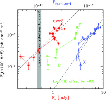
Correlation between the non-thermal UV flux (UVOT filter uvw2, subtracting the disc and the Lyα contributions), non-thermal optical flux (UVOT filter b, subtracting the disc contribution), non-thermal X-rays and the γ-ray flux. The grey vertical stripe indicates the contribution of the accretion disc plus the tail of the Lyα line entering in the uvw2 frequency range. The dashed lines are the linear fit to the γ-ray flux with the uvw2 and X-ray fluxes (see text).

Open in new tabDownload slide

The total time interval is the same shown in Fig. 1, i.e. about 1.5 months. The γ-ray flux correlates with both the UV–optical and X-ray fluxes, and the correlation is more than linear: for a total variation of a factor of ∼20 of F_γ, the optical–UV and the X-ray variability amplitude is a factor of ∼3–4. The vertical grey stripe indicates the flux contribution in the uvw2 UVOT filter due to the accretion disc emission according to our model plus the contribution from the tail of the Lyα line intercepted by the uvw2 filter.

Formally, a least-squares fit assuming a relation log F_γ=m log F_uvw2+q yields m = 1.567 and q=−5.026 (these are the values for the bisector of the correlations y=m₁x+q₁ and x=m₂y+q₂), with a chance probability P = 6.4 × 10⁻⁷.

The correlation with the X-ray flux, as illustrated in Fig. 2, seems to suggest the presence of an X-ray constant component contributing at a level of ∼ 5 × 10⁻¹¹ erg cm⁻² s⁻¹. On the other hand, the plotted data refer only to the 2009 November–December campaign, while the ‘low’ state (shown in Fig. 4) shows that there are states with lower X-ray and γ-ray fluxes (see Table 1 and Table 2). The suspected candidate for this behaviour is the synchrotron self-compton (SSC) component during the 2009 November–December period, as we will discuss in Section 5.1. Applying a least-squares fit to the data of Fig. 2, we find log F_γ = 2.267 log F_X+ 17.512 (again these are the bisector values) and a chance probability of P = 5 × 10⁻⁷.

The correlated variability in the three bands strongly suggests that the corresponding fluxes originate in the same region and by the same population of electrons. This supports the ‘one-zone’ models.

The fact that F_γ varies more than linearly with the optical–UV and the X-ray fluxes is interesting and, at first sight, surprising. Indeed the optical–UV is likely synchrotron emission, while the X-ray flux, having a shape much harder than the optical spectrum, belongs to the same HE hump as the γ-ray emission. We then expect that F_γ and F_X vary together, with F_γ∝F_X. Furthermore, if the γ-ray emission is produced by inverse Compton scattering with broad-line photons, produced externally to the jet – i.e. it is External Compton (EC) radiation – it is proportional to the number of the emitting electrons, as the synchrotron flux. Variations of the electron number should then result in F_γ∝F_opt. Finally, if the SSC process contributes substantially in the X-ray band, F_X is proportional to the square of the number density of the emitting electrons, and then we expect F_X∝F²_γ, just the opposite of what observed. A very similar behaviour has been observed for PKS 1502+106 (Abdo et al. 2010a).

More than linear and even more than quadratic variations of the HE γ-ray flux with respect to the X-ray flux have been already observed in TeV BL Lacs for relatively short (i.e. weeks) periods of time, as in Mkn 421 (Fossati et al. 2008) and PKS 2155−304 (Aharonian et al. 2009), but in these cases the X-ray emission belongs to the synchrotron part of the spectrum, while the γ-ray flux is probably SSC emission. Even so, it is not easy to explain a quadratic relation during the decaying phases of the light curves, because this implies short cooling time-scales (Katarzynski et al. 2005), leading Katarzynski & Walczewska (2010) to propose that the X-ray flux of the varying component must be diluted by the flux produced by another region.

In conclusion, we have that the γ-ray flux varies more than the flux at lower energies both in 3C 454.3 (and PKS 1502+106) and in the less powerful BL Lac objects, despite the large differences in the jet power and in the jet environment leading to different emission processes for the γ-ray photons (i.e. SSC for BL Lacs and EC for 3C 454.3 and other powerful FSRQs). While these similarities deserve further studies, we note here that for powerful blazars we have very short cooling times of the emitting electrons, even at low energies: this at least helps to explain the decaying phases of the light curves, that are instead a problem for TeV BL Lacs. For the specific case of 3C 454.3, we will suggest in the following the likely cause of F_γ varying more than F_X and F_opt, in terms of an inverse correlation between the dissipated power and the magnetic field.

3.1 Variability and cooling time-scales

Tavecchio et al. (2010) analysed in detail the entire light curve of 3C 454.3 in γ-rays, including the period of exceptional activity studied here. It is found that the minimum doubling time-scale is between 3 and 6 h (in our observer frame). This result has also been confirmed by Foschini et al. (2010), who studied another flare occurred in early 2010 April, comparable in flux but observed by Fermi/LAT in pointed mode, therefore with denser time coverage and enhanced statistics. From Fig. 2, we can see that also in X-rays (note the decrease at December 6 and at December 12) the variability time-scale is ∼1 d or shorter. This behaviour has two important consequences.

• The size of the emitting region must be compact, R < ct_varδ/(1 +z) ≈ 7 × 10¹⁵t_var,6h(δ/20) cm. As remarked in Tavecchio et al. (2010), this challenges models in which the dissipation region is at tens of parsecs from the black hole (see e.g. Jorstad et al. 2010), and instead favours models in which the dissipation occurs much closer.

• The cooling time t_cool≤t_var for electrons emitting at γ-ray and X-ray energies. This favours models in which the dissipation occurs in a region where the high density of photons can ensure a rapid cooling. Again, dissipation close to the black hole is favoured, where the BLR can provide a radiation energy density large enough to have t_cool < t_var even for electrons with random Lorentz factors of a few.

3.2 Contribution of the Lyα and of the accretion disc

At a redshift of z = 0.859, the Lyα emission line from the BLR is observed at 2260 Å, within the band of the uvm2 filter of UVOT (effective wavelength λ_eff = 2231Å; Poole et al. 2008).

In this source the line is bright (rest-frame equivalent width EW = 74 Å, according to the observations by Wills et al. 1995), and we wanted to check if it could explain the small excess in the uvm2 and uvw2 filters that is visible in the SED (Fig. 4). In Fig. 3, we show the 1900–2750 Å portion of the UV spectrum of 3C 454.3 observed by the GALEX satellite in 2008 October, together with the SED points observed in the UVOT filters and the corresponding transmission curves. All data have been dereddened with A_B = 0.46 and R_V = 3.1, following Raiteri et al. (2008) and assuming the extinction law from Cardelli et al. (1989). A small mismatch is apparent, but many factors can account for it, such as systematics in the flux measurement between the two instruments and the loose simultaneity of the observations performed with the two telescopes. Moreover, a quantitative study on this issue is far beyond the scope of this paper. Fig. 3 shows that the small bump in the portion of the SED observed by the UVOT filters can be partially due to the Lyα emission line shining the uvm2, and, at a lower level, the neighbouring filters, especially uvw2. This excess was well visible in all our UVOT pointings despite the larger level of the non-thermal contribution. Further, we tried to build a simple model for this portion of the spectrum, as the sum of three components:

• the Lyα emission line, modelled as a Gaussian profile, with σ and normalization obtained from a fit to the GALEX spectrum;

• the blue bump due to a ‘standard’ accretion disc, assumed constant (see Section 4);

• a variable power-law contribution, representing the synchrotron emission from the jet.

With these three components, we managed to reproduce the SED profile for each UVOT observation we considered. The excess in the uvm2 filter that we attributed to the Lyα line was compatible, within the uncertainties, with a constant contribution. This supports Raiteri et al. (2007) when they explain the smaller variability range in the UV band with respect to the optical and infrared (IR) as due to the presence of a blue, stable contribution, becoming more important (relative to the steep synchrotron non-thermal continuum) at higher frequencies. What we emphasize is the presence of two constant components: the accretion disc and the Lyα line.

3.3 The SED of 3C 454.3 at different epochs

In Fig. 4, we show the overall optical to γ-ray SED of 3C 454.3 at five different epochs during 2009 November and December and an additional one (‘low’) representative of a low γ-ray state (see Section 2). We can see the large variability amplitude of the γ-ray flux, whose spectrum is instead remarkably less variable, as noted also in Abdo et al. (2010b). Although it is somewhat harder in the ‘low’ state and on 2009 November 27, it is always characterized by a slope α_γ > 1[F(ν) ∝ν^−α], so that the peak of the γ-ray spectrum is at energies smaller than 100 MeV. On the other hand, the X-ray 0.2–10 keV slope and the Swift/BAT data points suggest that the peak cannot be much below 100 MeV.

As discussed above, we can see that the optical–UV flux varies, but less than the γ-ray flux. At low states, the accretion disc becomes ‘visible’ by flattening the spectrum. The presence of the accretion disc emission has been as noted by Raiteri et al. (2007) discussing observations in 2006–2007, which indicate that the disc produced a flux comparable with what is reported in Fig. 4.

As remarked before, also the X-ray flux varied much less than the γ-ray one during 2009 November–December. On the other hand, in the ‘low’ state, the X-ray flux is much lower (also with respect to the optical), and still very hard.

3.4 The mass of the black hole of 3C 454.3

Gu, Cao & Jiang (2001) estimated M = 4 × 10⁹M_⊙ for the mass of the black hole of 3C 454.3. They used the size of the BLR, R_BLR and the full width at half-maximum (FWHM) of the Hβ line equal to 2800 km s⁻¹ (Netzer et al. 1995). To derive the velocity of the clouds, they multiplied the FWHM value by a factor f = 1.5 (V=f V_FWHM), according to McLure & Dunlop (2001). The McLure & Dunlop f = 1.5 factor was empirically estimated assuming that the clouds belong to two components: one moving randomly and isotropically (that would give ⁠) and one distributed in a disc-like geometry. To derive the black hole mass through M=R_BLRV²G⁻¹, R_BLR was found using the relation of Kaspi et al. (2000):

1

where (λL_λ)_{5100 Å} is the luminosity of the continuum at 5100 Å (rest frame, corresponding to an observed wavelength of 9480 Å). For high-luminosity quasars, the more recent results of Kaspi et al. (2007), obtained using the C ivλ1549 line, yield

2

The observed luminosity at 2510 Å (corresponding to 1350 Å, rest frame) in a period of low state, not much contaminated by the non-thermal continuum, was λL_λ∼ 4 × 10⁴⁶ erg s⁻¹ (from the spectrum taken by the GALEX satellite reported in Fig. 3). This yields R_BLR∼ 6 × 10¹⁷ cm. The FWHM of the C iv line, according to Wills et al. (1995), is 3145 km s⁻¹. Assuming an isotropic velocity field, ⁠, the mass calculated through M=R_BLRV²G⁻¹ is M = 3.4 × 10⁸ M_⊙. Assuming f = 1.5, instead, we find M = 1.2 × 10⁹ M_⊙, in any case smaller than estimated by Gu et al. (2001). Since the continuum could in fact be contaminated by the non-thermal beamed contribution, these values should be considered as upper bounds. Furthermore, given the uncertainties in these relations, this estimate can give only a rough indication of the black hole mass. In the following, when modelling the SED, we will use M = 5 × 10⁸ M_⊙. In the general framework of our model, this is the black hole mass ensuring an observed minimum variability time-scale of ∼6 h, if the jet opening angle in its conical part is 0.1 rad, as assumed for all other blazars analysed in Ghisellini et al. (2010).

4 MODELLING THE SED

To model the SED we have used a relatively simple leptonic, one-zone synchrotron and inverse Compton model. This model, fully discussed in Ghisellini & Tavecchio (2009), has the following main characteristics.

We assume that in a spherical region of radius R, located at a distance R_diss from the central black hole, relativistic electrons are injected at a rate Q(γ) (cm⁻³ s⁻¹) for a finite time equal to the light crossing time R/c. For the shape of Q(γ), we adopt a smoothly broken power law with a break at γ_b:

3

The emitting region is moving with a velocity βc corresponding to a bulk Lorentz factor Γ. We observe the source at the viewing angle θ_v and the Doppler factor is δ = 1/[Γ(1 −β cos θ_v)]. The magnetic field B is tangled and uniform throughout the emitting region. We take into account several sources of radiation externally to the jet: (i) the broad-line photons, assumed to re-emit 10 per cent of the accretion luminosity from a shell-like distribution of clouds located at a distance R_BLR = 10¹⁷L^1/2_d,45 cm; (ii) the IR emission from a dusty torus, located at a distance R_IR = 2.5 × 10¹⁸L^1/2_d,45 cm; (iii) the direct emission from the accretion disc, including its X-ray corona. Furthermore, we take into account the starlight contribution from the inner region of the host galaxy and the cosmic background radiation, but these photon sources are unimportant in our case. We instead neglect, for simplicity, the contribution of a possible population of intracloud free electrons. This contribution would be important if the optical depth τ of these electrons became greater than the covering factor of the emitting line clouds, i.e. τ > 0.1, a rather large value. These free electrons would scatter and re-isotropize the entire disc flux, providing IR radiation, besides optical and UV. The final effect would be to broaden the HE hump, especially below its peak.

All these contributions are evaluated in the blob comoving frame, where we calculate the corresponding inverse Compton radiation from all these contributions, and then transform into the observer frame. For simplicity, the numerical code assumes an abrupt cut-off for the scattering cross-section, equal to the Thomson one for γhν_Lyα/m_ec² < 1 and zero above. This approximation provides acceptable results in the calculation of the inverse Compton scattering of the BLR (e.g. Tavecchio & Ghisellini 2008) and starts to fail only at the largest energies probed by LAT, at which scatterings in the full Klein–Nishina regime start to be important (see also Georganopoulos, Kirk & Mastichiadis 2001; Moderski et al. 2005, for a discussion on the importance of the full Klein–Nishina cross-section).

We calculate the energy distribution N(γ) (cm⁻³) of the emitting particles at the particular time R/c, when the injection process ends. Our numerical code solves the continuity equation which includes injection, radiative cooling and e^± pair production and reprocessing. Ours is not a time-dependent code: we give a ‘snapshot’ of the predicted SED at the time R/c, when the particle distribution N(γ) and consequently the produced flux are at their maximum.

For 3C 454.3, the radiative cooling time of the particles is short, shorter than R/c even for low-energetic particles. This implies that, at lower energies, the N(γ) distribution is proportional to γ⁻², while, above ⁠. The electrons emitting most of the observed radiation have energies γ_peak which is close to γ_b (but these two energies are not exactly equal, due to the curved injected spectrum).

The accretion disc component is calculated assuming a standard optically thick geometrically thin Shakura & Sunjaev (1973) disc. The emission is locally a blackbody, with a temperature profile given e.g. in Frank, King & Raine (2002). Since the optical–UV is the sum of the accretion disc and the jet non-thermal components, there is some degeneracy when deriving the black hole mass and the accretion rate, even in the lowest state, for which the disc is best visible. On the other hand, we can take as a guideline the value of the black hole mass derived in Section 4.1, implying then a very large accretion rate. We also note that in modelling the optical–UV region, one should also consider other thermal components, such as the other emission lines and the Balmer continuum from the BLR. However, all these components are expected to be much less bright than the Lyα emission line, included in the fit. It is also possible that the disc emission spectrum is different than that expected by the Shakura & Sunjaev model; however we use the latter, built on robust theoretical basis.

We model at the same time the thermal disc (and IR torus) radiation and the non-thermal jet emission. The link between these two components is given by the amount of radiation energy density (as seen in the comoving frame of the emitting blob) coming directly from the accretion disc or reprocessed by the BLR and the IR torus. This radiation energy density depends mainly on R_diss, but not on the adopted accretion rate or black hole mass (they are in any case chosen to reproduce the observed thermal disc luminosity).

By estimating the physical parameters of the source, we can calculate the power that the jet carries in the form of radiation (P_r), magnetic field (P_B), relativistic electrons (P_e) and cold protons (P_p) assuming one proton per electron. These powers are calculated according to

4

where U′ is the energy density of the ith component in the comoving frame.

4.1 Constraints on the model parameters

We briefly discuss the constraints that we can put on our modelling.

• The size R of the emitting region must be compact, in order to vary with the observed short time-scale. In the adopted model, this corresponds to a location of a jet dissipation region R_diss∼ct_varδ/[(1 +z)ψ]∼ 7 × 10¹⁶t_var,6h(δ/20)/ψ₋₁ cm, if the jet opening angle is ψ = 0.1 ψ₋₁.

• The short variability time-scale and the large disc luminosity imply R_diss < R_BLR: the dissipation occurs within the BLR.

• If so, the relevant radiation energy density is provided by the BLR photons, with energy density U′_BLR∼f_BLRL_dΓ²/(4πR²_BLRc). Setting f_BLR = 0.1 and using R_BLR = 10¹⁷L^1/2_d,45 cm, the resulting U′_BLR∼Γ²/(12π), i.e. the dependence on L_d and R_BLR drops out. As a consequence, the Lorentz factor of the electrons cooling in a time R/c is (U_B and U′_syn are the magnetic and the synchrotron energy densities):

  

  5

  Therefore the radiative cooling is efficient for all but the lowest energy electrons.

• The bulk Lorentz factor Γ and the Doppler factor δ are constrained by the observed superluminal motion at the very long baseline interferometry (VLBI) scale. Jorstad et al. (2005) find different components moving with different apparent velocities β_app, from a few to more than 20, for observations performed between 1998 and 2001, resulting in different bulk Lorentz factors (from 10 to 25) and different orientations (viewing angles from 2 to 4°), resulting in different Doppler factors (δ from 14 to 30). More recent observations by Lister et al. (2009) found β_app = 14.2 ± 0.8, consistent with the previous findings.

• The soft slope of the γ-ray spectrum and the hard slope of the X-ray spectrum constrain the peak of the HE component hν_c of the SED to lie below 100 MeV (but close to this value). For the EC process, the peak is made by the most relevant electrons scattering the Lyα seed photons. They must have a Lorentz factor γ_peak given by

  

  6

  This implies that the emission at and above the γ-ray peak is in fast cooling (i.e. that the cooling time is shorter than R/c).

• Since the bolometric luminosity is dominated by the γ-ray emission, this limits the injected power in the form of relativistic electrons. The fast cooling regime ensures that almost all the injected power is converted into radiation. We then have P′_inj≈L_γ/δ⁴.

• In general, the value of the magnetic field in the emitting region is derived by the level of the synchrotron emission. However the peak of the synchrotron spectrum, and hence its bolometric luminosity, lies in the unobserved mm–far-IR frequency range. A more robust constrain comes from the soft X-ray band, where we have the contribution of the EC and SSC components. Their spectrum is different (the SSC is softer). Increasing the magnetic field B increases the SSC component. The B field is then found by reproducing the observed flux and shape of the X-ray spectrum.

• The observed soft shape of the γ-ray and optical–UV spectra (once accounting for the contribution of the accretion emission, important in the low states) constraints the index s₂ of the energy distribution of the injected electrons. Since the cooling is almost complete (i.e. almost all electrons cool in R/c), the shape of the emitting distribution, below γ_peak, is ∝γ², almost independent of s₁ (if s₁<2). On the other hand, the details of the curvature around γ_peak and the distribution below γ_cool do depend on s₁. This index is then found by reproducing the X-ray spectrum (and the Swift/BAT point).

5 RESULTS

Fig. 4 shows the results of our modelling for the six simultaneous SEDs for different epochs, while Table 4 lists the used parameters. Fig. 5 shows the same SEDs and models, but extending the frequency axis to the radio band and showing some archival data, to put the SEDs analysed here in contest.

Table 4

Open in new tab

For all models, we have assumed a viewing angle and a bolometric luminosity of the accretion disc L_disc = 6.75 × 10⁴⁶ erg s⁻¹. The black hole mass is assumed to be M = 5 × 10⁸ M_⊙, so the disc luminosity is the 90 per cent of the Eddington value, and the mass accretion rate is ⁻¹ (assuming an efficiency η = 0.08). The size of the emitting blob, for the assumed distances R_diss from the black hole, is always ψR_diss, with ψ = 0.1. We assume that the 10 per cent of the disc luminosity is reprocessed by the BLR and re-emitted as broad lines at a distance R_BLR = 8.2 × 10¹⁷ cm for all models. Another 30 per cent of the disc luminosity is reprocessed and re-emitted as IR radiation by a torus, located at R_IR∼ 2 × 10¹⁹ cm. The minimum observed variability time-scale t_var is in hours and is defined as t_var=R(1 +z)/(cδ). Powers are in units of erg s⁻¹. Size and distances in units of 10¹⁵ cm. Magnetic field B in Gauss. Outflow mass rates in M_⊙ yr⁻¹.

	Low	06/11	27/11	01/12	02/12	03/12
Rdiss	132	156	174	150	173	174
P′inj	0.012	0.054	0.083	0.09	0.145	0.13
B	6.35	5.79	4.57	5.24	4.43	4.49
Γ	15	15	17	18	19.6	19.7
γb	400	340	800	600	350	430
γmax	2.0e3	3.4e3	2.8e3	3.0e3	2.8e3	3.0e3
s1	1.2	1.4	1.45	1.2	0.8	1.3
s2	3.4	4.0	3.9	4.3	3.5	3.4
Rdiss/Rs	880	1040	1160	1000	1150	1160
Rblob	13.2	15.6	17.4	15.0	17.6	17.7
γpeak	149	95.8	206.6	203	176	144
δ	24.5	24.5	26.4	27.3	28.4	28.5
tvar	5.0	5.9	6.1	5.1	5.7	5.8
log Pr	45.35	45.98	46.33	46.42	46.72	46.66
log Pp	47.08	47.97	48.11	48.01	48.09	48.37
log Pe	44.62	45.40	45.51	45.51	45.63	45.76
log PB	45.84	45.84	45.84	45.88	45.94	45.96
	0.14	1.08	1.33	1.01	1.08	2.09

	Low	06/11	27/11	01/12	02/12	03/12
Rdiss	132	156	174	150	173	174
P′inj	0.012	0.054	0.083	0.09	0.145	0.13
B	6.35	5.79	4.57	5.24	4.43	4.49
Γ	15	15	17	18	19.6	19.7
γb	400	340	800	600	350	430
γmax	2.0e3	3.4e3	2.8e3	3.0e3	2.8e3	3.0e3
s1	1.2	1.4	1.45	1.2	0.8	1.3
s2	3.4	4.0	3.9	4.3	3.5	3.4
Rdiss/Rs	880	1040	1160	1000	1150	1160
Rblob	13.2	15.6	17.4	15.0	17.6	17.7
γpeak	149	95.8	206.6	203	176	144
δ	24.5	24.5	26.4	27.3	28.4	28.5
tvar	5.0	5.9	6.1	5.1	5.7	5.8
log Pr	45.35	45.98	46.33	46.42	46.72	46.66
log Pp	47.08	47.97	48.11	48.01	48.09	48.37
log Pe	44.62	45.40	45.51	45.51	45.63	45.76
log PB	45.84	45.84	45.84	45.88	45.94	45.96
	0.14	1.08	1.33	1.01	1.08	2.09

Table 4

Open in new tab

For all models, we have assumed a viewing angle and a bolometric luminosity of the accretion disc L_disc = 6.75 × 10⁴⁶ erg s⁻¹. The black hole mass is assumed to be M = 5 × 10⁸ M_⊙, so the disc luminosity is the 90 per cent of the Eddington value, and the mass accretion rate is ⁻¹ (assuming an efficiency η = 0.08). The size of the emitting blob, for the assumed distances R_diss from the black hole, is always ψR_diss, with ψ = 0.1. We assume that the 10 per cent of the disc luminosity is reprocessed by the BLR and re-emitted as broad lines at a distance R_BLR = 8.2 × 10¹⁷ cm for all models. Another 30 per cent of the disc luminosity is reprocessed and re-emitted as IR radiation by a torus, located at R_IR∼ 2 × 10¹⁹ cm. The minimum observed variability time-scale t_var is in hours and is defined as t_var=R(1 +z)/(cδ). Powers are in units of erg s⁻¹. Size and distances in units of 10¹⁵ cm. Magnetic field B in Gauss. Outflow mass rates in M_⊙ yr⁻¹.

	Low	06/11	27/11	01/12	02/12	03/12
Rdiss	132	156	174	150	173	174
P′inj	0.012	0.054	0.083	0.09	0.145	0.13
B	6.35	5.79	4.57	5.24	4.43	4.49
Γ	15	15	17	18	19.6	19.7
γb	400	340	800	600	350	430
γmax	2.0e3	3.4e3	2.8e3	3.0e3	2.8e3	3.0e3
s1	1.2	1.4	1.45	1.2	0.8	1.3
s2	3.4	4.0	3.9	4.3	3.5	3.4
Rdiss/Rs	880	1040	1160	1000	1150	1160
Rblob	13.2	15.6	17.4	15.0	17.6	17.7
γpeak	149	95.8	206.6	203	176	144
δ	24.5	24.5	26.4	27.3	28.4	28.5
tvar	5.0	5.9	6.1	5.1	5.7	5.8
log Pr	45.35	45.98	46.33	46.42	46.72	46.66
log Pp	47.08	47.97	48.11	48.01	48.09	48.37
log Pe	44.62	45.40	45.51	45.51	45.63	45.76
log PB	45.84	45.84	45.84	45.88	45.94	45.96
	0.14	1.08	1.33	1.01	1.08	2.09

	Low	06/11	27/11	01/12	02/12	03/12
Rdiss	132	156	174	150	173	174
P′inj	0.012	0.054	0.083	0.09	0.145	0.13
B	6.35	5.79	4.57	5.24	4.43	4.49
Γ	15	15	17	18	19.6	19.7
γb	400	340	800	600	350	430
γmax	2.0e3	3.4e3	2.8e3	3.0e3	2.8e3	3.0e3
s1	1.2	1.4	1.45	1.2	0.8	1.3
s2	3.4	4.0	3.9	4.3	3.5	3.4
Rdiss/Rs	880	1040	1160	1000	1150	1160
Rblob	13.2	15.6	17.4	15.0	17.6	17.7
γpeak	149	95.8	206.6	203	176	144
δ	24.5	24.5	26.4	27.3	28.4	28.5
tvar	5.0	5.9	6.1	5.1	5.7	5.8
log Pr	45.35	45.98	46.33	46.42	46.72	46.66
log Pp	47.08	47.97	48.11	48.01	48.09	48.37
log Pe	44.62	45.40	45.51	45.51	45.63	45.76
log PB	45.84	45.84	45.84	45.88	45.94	45.96
	0.14	1.08	1.33	1.01	1.08	2.09

Figure 5

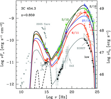
Same as Fig. 4, but extending to radio frequencies and showing also archival data (in light grey), including the optical fluxes achieved during the 2005 optical flare, the 2000 June 5–6 BeppoSAX spectrum (Tavecchio et al. 2002) and the EGRET spectrum of 1992 January (Nandikotkur et al. 2007). Note that (i) during the optical flare of 2005, the optical flux reached a brighter state than in 2009 November–December; (ii) the low Fermi/LAT state is at a lower level than detected by EGRET and (iii) that the X-ray flux and spectrum detected by Swift/XRT for the ‘low’ state superpose exactly to the BeppoSAX data.

Open in new tabDownload slide

The model successfully reproduces the data from the optical to the γ-ray band, using the guidelines explained in Section 4.1. The large variations of the γ-ray luminosity are obtained by mainly varying the power injected in relativistic electrons (by a factor of 10 from the ‘low’ to the highest state, and by a factor of 3 in the restricted period from November 6 to December 2), and the bulk Lorentz factor (from 15 to 20). These are the main changes. Besides them, there are minor changes in the location of the dissipation region (hence, in the size of the emitting region) by less than a factor of 1.4, and in the parameters of the injected electron distribution (i.e. γ_b changes by a factor of ∼2, and also s₁ changes somewhat). These changes are required to fit the X-ray spectrum, while the changes in the s₂ parameter are necessary to account for the (small) changes of the γ-ray and the optical–UV spectra. Although minor, these changes have a relatively strong impact on the total jet power, because γ_b and s₁ control the total amount of electrons present in the source, thus also the number of cold protons, if we assume one proton per electron. Indeed, the maximum value of P_p is obtained on December 3, not at the maximum of the γ-ray flux (occurring at December 2, when there is also the maximum value of P′_inj).

As explained in Section 4.1, the value of the magnetic field is mainly derived to adequately fit the X-ray spectrum, rather than the synchrotron optical–UV spectrum and flux level. Fig. 4 shows the contributions of the SSC and EC components for the SED of November 6. They intersect at ∼1 keV, with the SSC dominating below, and the EC above. A similar decomposition has been adopted in Vercellone et al. (2010) for another epoch (see their fig. 19, showing also the contribution of the accretion disc radiation to the optical–UV flux).

Fig. 5 shows that during the optical flare of 2005 the optical flux reached a brighter state than in 2009 November–December. There was no γ-ray facility in orbit in 2005, so we do not know the γ-ray flux during the optical flare, interpreted by Katarzynski & Ghisellini (2007; see also Ghisellini et al. 2007) as a dissipation event occurring relatively close to the black hole, where the magnetic energy density can be of the same order of the radiation energy density as seen in the comoving frame. In this case L_syn∼L_EC∼L_γ, and we do not need an extraordinary increase of the total power budget to explain this extraordinary optical flare that can occur without a corresponding large increase of the γ-ray flux (and the bolometric one; in this sense the model can be thought as ‘economic’, i.e. assuming the lowest possible power budget). On the contrary, the 2009 γ-ray flare does change the bolometric luminosity by a large factor, without inducing a correspondingly dramatic increase of the optical flux. The results of the modelling presented here explain this behaviour by having a larger power dissipated in regions more distant than in the 2005 flare, with relatively smaller magnetic field and larger bulk Lorentz factors.

Fig. 5 also shows that the ‘low’Fermi/LAT state is lower than the γ-ray flux detected by EGRET in January 1992 and that the X-ray flux and spectrum detected by Swift/XRT for the ‘low’ state superpose exactly to the BeppoSAX data of 2000 June 5–6 (discussed in Tavecchio et al. 2002).

5.1 γ-ray versus X-ray and γ-ray versus optical flux correlations

In Section 3, we showed that the γ-ray flux varies almost quadratically with the optical and X-ray fluxes. In the framework of synchrotron + EC model, modest variations of the synchrotron flux accompanied by large variations of the EC flux imply that the magnetic field must vary oppositely with the observed bolometric power (i.e. the γ-ray luminosity, in this case). Another way to have more than linear variations (but not quadratic) is to vary Γ, that would result in L_EC∝L^3/2_syn (this relation, valid considering frequency integrated luminosities, remains valid in restricted energy ranges if the EC and synchrotron peaks do not move).

Fig. 6 illustrates the specific way of our modelling to have the observed L_γ∝L²_opt correlation. The figure shows how B, Γ and R_diss depend on the observed L_γ, and how B depends on the product ΓR_diss. We can see that B inversely correlates with L_γ, while Γ and R_diss, instead, correlate positively. These makes B to be almost perfectly proportional to (ΓR_diss)⁻¹. Since P_B∝[R_dissΓB]², we have that the Poynting flux at R_diss is approximately constant for all the considered states.

Figure 6

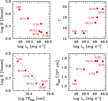
Top: the magnetic field B (left) and the bulk Lorentz factor Γ (right) as a function of the γ-ray luminosity L_γ for the six different SED plotted in Fig. 4. Bottom left: the magnetic field B as a function of ΓR_diss. Bottom right: R_diss as a function of L_γ.

Open in new tabDownload slide

To summarize, the large variation in the γ-ray flux accompanied by much more modest variations of the optical is explained by a magnetic field that decreases when the observed L_γ increases. This is accomplished, in our model, by having larger R_diss and Γ for larger L_γ and jet powers, and by having instead a quasi-constant Poynting flux in the emission region. By the same argument, we can explain the F_γ–F_X correlation, since the contribution of the SSC component to the X-rays becomes relatively more important for lower states, making the SSC X-ray flux to decrease much less than the γ-ray one.

However, the quasi-constancy of P_B may be partly a coincidence, and not the outcome of a fundamental process. This is because it is very likely that the Poynting flux P_B,0 at the start of the jet is the prime cause of the acceleration of the jet itself. In this case, since we find that the total jet power does change, P_B,0 should change as well, and yet have the same value when arriving at R_diss. What can happen is that a stronger P_B,0 implies a larger final Γ, achieved at a larger distance z (i.e. we can have Γ∝z^1/2 as in Vlahakis & Königl 2004). This means that a larger P_jet∼P_B,0 is achieved, but since both R_diss and Γ are larger, P_B at the dissipation region may vary much less than P_B,0∼P_jet∝L_γ.

5.2 The power of the jet

It is interesting to investigate if the extraordinary γ-ray flare corresponds to a real enhancement of the power carried by the jet or if originates by an enhanced efficiency in converting the jet power into radiation, or if is due to an increased Doppler factor δ, making the observed flux to increase even if the jet power remains constant. The nearly model-independent quantity connected to the jet power is P_r, the power that the jet spends to produce the radiation we see. Using U′_rad=L′/(4πR²c), we can rewrite equation (4) as

7

where L is the total observed non-thermal luminosity (L′ is in the comoving frame) and U′_rad is the radiation energy density produced by the jet (i.e. excluding the external components). The last equality assumes θ_v∼ 1/Γ. This quantity is almost model-independent, since it depends only on the adopted δ, that can be estimated also by other means, namely superluminal motions. In Table 4 we list the values of P_r for the different states. The maximum is on December 2, the day of the maximum L_γ, when P_r = 5.2 × 10⁴⁶ erg s⁻¹. This value can be compared with the accretion luminosity, that we assumed constant during the entire period and equal to L_d = 6.75 × 10⁴⁶ erg s⁻¹. The power P_r can be considered as a very robust lower limit to the total jet power P_jet=P_B+P_e+P_p. If the entire P_jet is used to produce the radiation we see (i.e. P_jet=P_r), then the jet would necessarily decelerate and there would be no VLBI superluminal knots, nor any extended radio emission.

Table 4 lists also the value if P_B and P_e. They are smaller than P_r. The fact that P_e < P_r may seem strange at first sight, since the radiation is produced by the electrons, so how can they have less power that what they transform in radiation? The answer is that the radiative cooling time is shorter than R/c, so electrons need to be injected continuously, at least for a time R/c. To estimate P_e, we count electrons (and their energy) forming the N(γ) (cm⁻³) energy distribution after solving the continuity equation, not the ones injected. An example can clarify this point: assume to inject the same energy distribution Q(γ) (cm⁻³ s⁻¹). In case A the radiative cooling is strong, in case B it is weak. The particle density N(γ) is always proportional to ⁠, therefore in case A, N(γ) is smaller than in case B. This despite the fact that in case A we have produced more radiation, since the cooling is stronger.

This implies that there must be a ‘reservoir’ of power able to energize electrons that in turn produce P_r. The simplest solution is to assume that this ‘reservoir’ is provided by protons. The listed values of P_p assume one proton per electron. The implication is that electron–positron pairs cannot be energetically dominant, even if we cannot exclude that they outnumber primary electrons (but not by a large factor). For a more detailed discussion about this point, see Sikora & Madejski (2000) and Celotti & Ghisellini (2008). We summarize here the arguments in Celotti & Ghisellini (2008). If pairs are dynamically important, they must outnumber protons and also the emitting leptons by a large factor. Although possible in principle, this solution poses the problem of the origin of this large number of pairs. If they have been created in the same emitting region (e.g. by γ–γ collisions), then we should see (i) a cut-off in the spectrum and (ii) some reprocessed radiation in X-rays (since the pairs are born relativistic). The level of this reprocessed radiation must be of the same order of the absorbed luminosity (i.e. it is large and should be well visible). If, instead, the pairs are created from the start, we can calculate how many we need. In powerful sources (as 3C 454.3) this number corresponds to an initial pair optical depth greater than unity. If initially cold, the pairs quickly annihilate, and the surviving ones are not enough (to be dynamically important). If they are hot, they emit. At the start of the jet, close to the accretion disc, the radiation energy density and the magnetic field make them to cool very rapidly. So they become cold, and annihilate (besides producing radiation we do not see).

Assuming then that P_p is a good proxy for the real P_jet, we see that during 2009 November and December the jet power varied only by a factor of 2, while L_γ varied by a factor of ∼10. This implies that the jet became more efficient in transforming its power into radiation, rather than becoming more powerful. For the ‘low’ state, instead, the estimated value of P_p∼ 10⁴⁷ erg s⁻¹ is a factor of 10 less than in November 27, with L_γ being a factor of 4 weaker. To summarize, the total excursion (from ‘low’ state to 2009 December 3) of P_p is factor of 20, not very different from the total amplitude of L_γ (factor of ∼30). But restricting the period from November 6 to December 3, the jet power is quasi-constant, while L_γ varied by a factor of 10.

5.3 Jet power versus disc luminosity

The disc luminosity is L_d = 6.7 × 10⁴⁶ erg s⁻¹, comparable to P_r. The jet power must be greater than P_r and therefore greater than L_d. This is one of the most important outcomes of having followed 3C 454.3 during its major γ-ray flare.

Table 4 lists the value of the outflowing mass rate, estimated through ⁠. Since Γ varies moderately (between 15 and 20) while P_p varies by a factor of 10, we have that also varies by an order of magnitude considering the entire time-span, and only by a factor of 2 in 2009 November–December. In this period, it is of the order of 1 solar mass per year. We can compare this value with the accretion mass rate ⁠, that we can derive through ⁠. Assuming η = 0.08, a disc luminosity L_d = 6.75 × 10⁴⁶ erg s⁻¹ gives ⁻¹, about a factor of 10 greater than ⁠.

If the disc emits at a constant level, with a constant ⁠, we are forced to conclude that the link between the accretion rate and the jet power is not determined by ⁠, or, rather, that this is not the only important quantity in producing P_jet. For the ensemble of bright FSRQs detected by Fermi, in fact, the disc luminosity does correlate with P_jet, even taking out the effect of a common redshift dependence in the two quantities (see Fig. 7 and the discussion in Ghisellini et al. 2010). Since the spin of the black hole of 3C 454.3 is constant, the likely quantity that modulates P_jet in 2009 November–December is the value of the magnetic field in the vicinity of the black hole horizon. If we assume that P_B,0=P_jet at the Schwarzschild radius R_S, the magnetic field must be

8

In turn, we can check if the magnetic energy density B²₀/(8π) can be equated to ρc², the mass energy density of the accreting matter close to the Schwarzschild radius. We can write

9

where V_R is the radial infalling velocity and 2H is the total height of the disc at the Schwarzschild radius. The above equation shows that if ρc²∼B²₀/(8π) and P_jet/L_d∼ 10, then β_R(H/R) ∼ 0.3, i.e. not an unreasonable value.

Figure 7

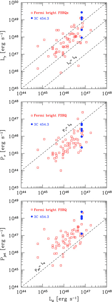
The observed γ-ray luminosity L_γ (top panel), the power P_r spent by the jet to produce the radiation we see (mid panel) and the total jet power P_jet (botton panel) as a function of the accretion disc luminosity L_d. The filled circles correspond to the six states of 3C 454.3 analysed in this paper, while the empty squares correspond to all the FSRQs detected in the first three months of the Fermi/LAT all-sky survey analysed by Ghisellini et al. (2010).

Open in new tabDownload slide

5.4 Is 3C 454.3 exceptional?

We finally ask if 3C 454.3 is exceptional, or instead if there are other blazars reaching comparable values of L_γ and of L_γ/L_d. To answer, we can compare the flaring state of 3C 454.3 with all blazars of known redshift of the first three months Fermi/LAT all-sky survey (Abdo et al. 2009c), analysed in Ghisellini et al. (2010), as done in the top panel of Fig. 7. We alert the reader that in Ghisellini et al. (2010) we have considered the averageγ-ray flux. Had we considered the peak flux values there would be a few FSRQs of L_γ even greater than 3C 454.3 in high state (one example is PKS 1502+102; Abdo et al. 2010a). In this respect, we can conclude that 3C 454.3 is not the most extreme blazar; its unprecedented γ-ray flux is due to its relative vicinity in comparison to other FSRQs. The same occurs in the planes P_r–L_d and P_jet–L_d (mid- and bottom panels of Fig. 7); there are other sources whose three months averaged P_r and P_jet are comparable to 3C 454.3.

6 CONCLUSIONS

The study of the strong γ-ray flare of 3C 454.3, together with the good coverage at X-ray and optical–UV frequencies provided by Swift allowed to investigate several issues about the physics of the jet of this blazar. In Tavecchio et al. (2010), we analysed the behaviour of the 1.5-yr Fermi/LAT light curve, finding episodes of very rapid variations, with time-scales between 3 and 6 h both during the rising and the decaying phases. This implies a very compact emitting region, suggesting that the dissipation zone is not too far from the black hole, and that cooling times are shorter than the variability time-scales. This in turn suggests that the dissipation region lies within the BLR, at about 1000 Schwarzschild radii.

We have revisited the estimate of the mass of the black hole of 3C 454.3, finding a smaller value than found by Gu et al. (2001). Since in our model the mass of the black hole sets the scales of the disc+jet system, a smaller mass helps to have a more compact emitting region, that can vary on shorter time-scales.

The optical, X-ray and γ-ray fluxes correlate. This supports one-zone models. The γ-ray flux varies quadratically (or even more) with the optical and X-ray fluxes. By modelling the optical to γ-ray SED with a one-zone synchrotron+inverse Compton leptonic model, we can explain this behaviour if the magnetic field is slightly fainter when the overall jet luminosity is stronger.

The power that the jet spent to produce the peak γ-ray luminosity is of the same order than the accretion disc luminosity. Although the jet power correlates with the accretion luminosity considering the ensemble of bright FSRQs detected by Fermi, 3C 454.3 probably varied its jet power while maintaining a constant accretion luminosity. This implies that the modulation of the jet power may not be due to variations of the accretion rate, but is probably due to variations of the magnetic field close to its black hole horizon.

We thank the referee for useful criticism. We acknowledge the use of public data from the Swift data archive. This research has made use of data obtained from the High Energy Astrophysics Science Archive Research Center (HEASARC), provided by NASA's Goddard Space Flight Center through the Science Support Center (SSC). Use of public GALEX data provided by the Multimission Archive at the Space Telescope Science Institute (MAST) is also acknowledged. This work was partially financed by a 2007 COFIN–MiUR grant and by ASI grant I/088/06/0.

REFERENCES