


Abstract
Deep, wide, near-infrared imaging surveys provide an opportunity to study the clustering of various galaxy populations at high redshift on the largest physical scales. We have selected 1 < z < 2 extremely red objects (EROs) and 1 < z < 3 distant red galaxies (DRGs) in SA22 from the near-infrared photometric data of the UKIDSS Deep eXtragalactic Survey and gri optical data from the Cerro Tololo Inter-American Observatory covering 3.3 deg2. This is the largest contiguous area studied to sufficient depth to select these distant galaxies to date. The angular two-point correlation functions and the real-space correlation lengths of each population are measured and show that both populations are strongly clustered and that the clustering cannot be parametrized with a single power law. The correlation function of EROs shows a double power law with the inflection at ∼0.6–1.2 arcmin (0.6–1.2 h−1 Mpc). The bright EROs (K < 18.8) show stronger clustering on small scales but similar clustering on larger scales, whereas redder EROs show stronger clustering on all scales. Clustering differences between EROs that are old passively evolved galaxies and dusty star-forming galaxies, on the basis of their J −K colour, are also investigated. The clustering of r −K EROs is compared with that of i −K EROs and the differences are consistent with their expected redshift distributions. The correlation function of DRGs is also well described by a double power law and consistent with previous studies once the effects of the broader redshift distribution our selection of DRGs returns are taken into account. We also perform the same analysis on smaller subfields to investigate the impact of cosmic variance on the derived clustering properties. Presently, this study is the most representative measurement of the clustering of massive galaxies at z > 1 on large scales.
1 INTRODUCTION
The Lambda cold dark matter paradigm predicts that the small-scale structure has developed by accretion and mergers within the large-scale structure generated by primordial mass fluctuations. In addition, the galaxies tracing this structure are themselves embedded and have evolved in the dark matter haloes (White & Frenk 1991). The halo properties, such as abundance, distribution and density profile, depend on the mass of halo (Cooray & Sheth 2002). As a result, the formation and evolution of galaxies is affected by the halo mass (Eke et al. 2004; Baugh 2006). Therefore, the clustering properties of galaxies can be related to the distribution of dark matter haloes, and hence offer an important insight into the relationship between the halo and the galaxies within it. For instance, Wake et al. (2008) used correlation functions and halo models to demonstrate that luminous red galaxies (LRGs) are frequently located in the centre of the most massive dark matter haloes, and that changes in their small-scale clustering with redshifts can constrain LRG–LRG merger rates. At higher redshifts, Mo & White (2002) pointed out that haloes of given mass are expected to be more clustered from simulations. Observationally, Foucaud et al. (2010) have demonstrated that galaxies with higher stellar masses are more clustered, and galaxies with a fixed stellar mass are also more clustered at a higher redshift. Hartley et al. (2010) have also shown that passive, red galaxies are more clustered than star-forming, blue galaxies of similar absolute magnitudes at 0.5 < z < 3.0. Quadri et al. (2008) found that a double power law was required to describe the correlation function of DRGs at 2 < z < 3, but were unable to fit their clustering measurement and space density simultaneously using the halo model. Tinker, Wechsler & Zheng (2010) showed that using a more realistic halo model they could better fit this clustering measurement, but they still required that the observed region be a more clustered part of the universe than is typical. However, most observational studies of clustering and the halo model have concentrated on relatively low redshifts (z < 1), so their evolution has been poorly constrained. With the advent of large near-infrared (near-IR) surveys, it is now possible to apply these techniques to more distant galaxies. The study of the angular clustering of z > 1 galaxies is particularly powerful as the near-constant angular diameter distance in the 1 < z < 3 range means that the angle and comoving distance are much more closely linked than at a lower redshift. Therefore, any characteristic distance (halo transition or sound horizon at last recombination) will translate to a small range in angle.
Many colour criteria have been used to select high-redshift galaxies. One of the crudest but most direct methods is to select galaxies with a large colour difference between optical and IR wavelengths (I −K > 4) (Elston, Rieke & Rieke 1988) to select extremely red objects (EROs). This technique preferentially selects the most massive galaxies at z > 1, which tend to be dominated by an evolved stellar population with a pronounced 4000 Å break. However, the spectra of EROs show evidence for a significant population of dusty, star-forming galaxies (Pozzetti & Mannucci 2000; Cimatti et al. 2002; Roche et al. 2002; Smail et al. 2002; Cimatti et al. 2003; Moustakas et al. 2004; Sawicki et al. 2005; Simpson et al. 2006; Conselice et al. 2008; Kong et al. 2009). EROs are strongly clustered (Daddi et al. 2000; Roche et al. 2002; Roche, Dunlop & Almaini 2003; Brown et al. 2005; Kong et al. 2006, 2009) and reside in massive dark matter haloes (Gonzalez-Perez et al. 2009).
Alternatively, a large near-IR colour difference, J −K > 2.3, can be used to select distant red galaxies (DRGs) (Franx et al. 2003) that are predominantly at z > 2. As with EROs, this simple colour cut selects galaxies with a range of redshifts (Lane et al. 2007; Quadri et al. 2007) and both dusty star-forming and passive galaxies (Labbé et al. 2005; Papovich et al. 2006). DRGs are also highly clustered (Grazian et al. 2006; Foucaud et al. 2007). Perhaps the most striking evidence for clustering of high-redshift galaxies is the angular clustering of Herschel SPIRE sources presented in Cooray et al. (2010), where the large-scale clustering and its distinct curvature are unambiguously detected for z > 1 far-infrared (FIR) selected galaxies that are presumably the progenitors of present-day massive, early-type galaxies from the similarity of their clustering properties.
The addition of a third photometric data point can improve the discrimination of high-redshift galaxy selection. For instance, for galaxies with a strong ultraviolet continuum, Steidel & Hamilton (1992) used an optical colour criterion to identify Lyman break galaxies at z > 3 and Adelberger et al. (2004) used the same filter system but selected galaxies at z ∼ 1.7 and 2.3, termed BM/BX galaxies. The broadest photometric selection method was suggested by Daddi et al. (2004), using the B, z and K filters to identify star-forming and passively evolved galaxies at z > 1.4.
With all of these photometric selection methods, the small field of view of imaging cameras has hampered the accurate measurement of large-scale clustering. In particular, the lack of wide-field near-IR instruments has prevented the detection of distant, passive galaxies, since the bulk of their emission is redshifted to longer wavelengths. However, new wide and deep near-IR surveys now provide an opportunity to investigate the clustering properties of galaxies at high redshift. In this paper, we use the wide contiguous near-IR data from 5th Data Release (DR5) of the Deep eXtragalactic Survey (DXS), which is the subsurvey of the UK Infrared Telescope Infrared Deep Sky Survey (UKIDSS) (Lawrence et al. 2007), in conjunction with gri optical data from the Cerro Tololo Inter-American Observatory (CTIO) 4 m to measure the clustering properties of EROs and DRGs, and discuss the clustering properties with various criteria.
In Section 2, we describe the compilation of UKIDSS DXS and optical data for the SA22 field. The analysis method for near-IR and optical data and determining clustering properties are then described in Section 3. The results are presented in Section 4 and discussed in Section 5. Unless otherwise noted, the photometry is quoted in the Vega scale. We also assume Ωm = 0.27, Λ = 0.73 and H0 = 71 km s−1 Mpc−1.
2 OBSERVATION
2.1 UKIDSS DXS
The UKIDSS began in 2005 and consists of five subsurveys covering various areas and depths (Lawrence et al. 2007). The UKIDSS uses the Wide Field Camera (WFCAM, Casali et al. 2007) mounted on the UK Infrared Telescope (UKIRT). Of the five subsurveys, the DXS is a deep, wide survey mapping 35 deg2 with 5σ point-source sensitivity of J ∼ 22.3 and K ∼ 20.8. It is comprised of four fields and aims to create photometric samples at z ∼ 1–2.
The WFCAM is composed of four Rockwell Hawaii-II 2K × 2K array detectors (Casali et al. 2007). The pixel scale is 0.4 arcsec pixel−1, so the size of each detector is 13.7 × 13.7 arcmin2. The relatively large pixel scale can lead to an undersampled point spread function (PSF). To avoid this problem, microstepping is applied. In addition, there are gaps between detectors and the width is similar to the size of a detector. Therefore, four exposures are needed to make a contiguous image, that is, 4 × 4 image tiling 0.8 deg2.
In this study, we deal with ∼3.3 deg2 SA22 field centred on  (J2000) from UKIDSS DR5. Since it is composed of four 0.8-deg2 fields from DXS SA22 1 to 4, there is a 16-point mosaic to cover the field. The DXS SA22 1 corresponds to the south-west part of our field, and SA22 2, 3 and 4 correspond to the south-east, north-east and north-west parts, respectively. Seeing conditions of all images were ∼0.9 arcsec at J and ∼0.8 arcsec at K.
2.2 Optical data
Optical gri images were obtained from the 4-m Blanco Telescope in the CTIO in 2006 September as a complement to the DXS as the SA22 field lacked any wide-field optical imaging. The observations were performed by Mosaic II CCD composed of eight 2K × 4K detectors. Each exposure covers 36 × 36 arcmin2, and nine fields were observed to map ∼3.3 deg2 UKIDSS DXS SA22 field. Total exposure times are 1800 s for g, 3000 s for r and 5400 s for i. In addition, five- or nine-point dithering methods were applied for g, r and i, respectively. The seeing was 1–2 arcsec for g and 1–1.5 arcsec for r and i.
3 ANALYSIS METHODS
3.1 UKIDSS DXS
The UKIDSS standard pipeline creates a catalogue by merging detected objects for each array. However, Foucaud et al. (2007) pointed out that creating a contiguous image before extracting the catalogue is more helpful to optimize depths in overlap regions and to make a homogeneous image. There are also some known issues that require particular care with analysing WFCAM data. Dye et al. (2006) discussed various artefacts of the UKIDSS Early Data Release (EDR), including internal reflections and electronic cross-talk. The former have been eradicated by additional baffling and restricting the observations with respect to the Moon angle, but the latter still have to be removed. Cross-talk is straightforward as each cross-talk feature is a fixed number of pixels from a bright star and can hence be flagged (see below). The standard CASU detection pipeline is not optimized for galaxy photometry, so we choose to create our own photometric catalogues from mosaicked images.
First, four contiguous images were created from the reduced images including astrometric and photometric information from the UKIDSS standard pipeline. As mentioned above, we used ∼3.3 deg2 field, which is composed of four 0.8-deg2 fields. Instead of creating one large contiguous image, four separate images were made, since the integration time for each exposure was changed from 5 to 10 s after the first UKIDSS observing period. Before stacking, the flux scale of each array was calculated by using the zeromag from the UKIDSS standard pipeline. The SWarp software, which is a resampling and stacking tool (Bertin et al. 2002), was run to stack the images. A weight map was created by SWarp and bad regions at the detector edges or around saturated stars were masked by visual inspection.
Secondly, objects were extracted from these contiguous images by running SExtractor (Bertin & Arnouts 1996). To measure colours of objects, the flux has to be measured for the same part of each object. Therefore, the J-band image was transformed into the K-band image frame by the iraf tasks, GEOMAP and GEOTRAN, used to calculate a transforming equation and transform the images, respectively. Also, in order to minimize the fraction of spurious objects, various combinations of thresholds and detection areas were tested. Finally, the K-band image was used as a detection image to detect faint objects in the other bands. Colours were calculated using 2-arcsec aperture magnitudes for each band, and total magnitudes in K were measured using the SExtractor AUTO magnitude. A photometric calibration was applied by using the calibrated aperture magnitude of the point-source catalogue from the UKIDSS standard pipeline, which was calibrated from the Two-Micron All-Sky Survey (Skrutskie et al. 2006).
Thirdly, spurious objects, such as cross-talk images and diffraction spikes, were removed. The cross-talk images were located at multiples of 256 pixels from bright objects (Dye et al. 2006). We selected cross-talk candidates related to bright stars (K < 16) by position. All potential cross-talk images from the brightest stars (K < 13) were removed. However, those from fainter stars (13 < K < 16) contain a fraction of real objects. Fortunately, since cross-talk images of fainter hosts accompany dark spots around them, these spots were used to determine whether candidates are cross-talk images or real objects. In addition, spurious objects detected on diffraction spikes were selected by position from bright stars and removed. In total, 6 per cent of the objects were removed as spurious objects using these methods. We detected 303 473 bona fide objects from the masked 3.07-deg2 field.
Finally, a completeness test was performed to check the photometric quality. We randomly added 1000 artificial stars into each image and ran SExtractor again with the same parameters. This process was repeated 10 times with different artificial stars. Fig. 1 shows the completeness of each field for J (top panel) and K (bottom panel). The horizontal and vertical lines indicate the 90 per cent completeness and the design depth of the DXS, respectively. The completeness of DXS SA22 4 at J is significantly lower than others. This was caused by the relatively high background value in this field. However, the other fields successfully reach the target magnitude limit in both bands.
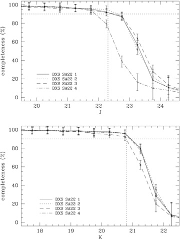
Completeness test result. The horizontal and vertical lines indicate 90 per cent completeness and the target limiting magnitude of the DXS, respectively.
3.2 Optical data
We followed the standard image reduction sequence for mosaic CCD, namely bias subtraction, flat-fielding by dome and sky flat images, masking bad pixels and removing cross-talk artefacts and cosmic rays. The USNO-A2 catalogue was used to improve the astrometric solution for each field. This solution was also applied to project images so they had the same scale and astrometry, using the iraf tasks GEOMAP and GEOTRAN. Finally, these projected images were combined by using median values and exposure maps were used as a weight map.
As with the near-IR data, colours of galaxies have to be measured from the same part of each object. Therefore, images for the same field have to be matched to have the same seeing. To do this, the better seeing images were degraded using the PSFMATCH task in iraf. The daophot package was used to select unsaturated stars and to create PSF kernels. These kernels were then used to degrade better seeing images to the worst seeing.
In order to detect objects and measure fluxes, the same strategy used for the near-IR data was applied. SExtractor (Bertin & Arnouts 1996) was run in dual mode. The i-band image was used as the detection image. Saturated stars and their haloes were masked in the weight image to remove unreliable objects. Various threshold values were tested and the value minimizing spurious objects was selected. Finally, since the seeing of the CTIO imaging was worse than the DXS, ISO and AUTO magnitude were used to estimate colours instead of the aperture magnitude and total magnitude.
Photometric calibration was performed using the Sloan Digital Sky Survey (SDSS, York et al. 2000) catalogue. Aperture colours from SExtractor were calibrated to those of the SDSS, and the absolute flux calibration was determined using the total magnitudes in i with respect to those in the SDSS. Finally, we removed unreliable photometric results using a magnitude cut. To remove saturated stars, objects brighter than i < 17.6 were replaced by the equivalent SDSS data. In addition, since the number density of objects decreases sharply at i > 24.6 and the completeness computed from artificial stars is ∼85 per cent at i = 24.6, we extracted only objects brighter than i = 24.6. A total of 302 402 objects were extracted for the masked 2.45-deg2 optical catalogue.
3.3 Matching optical and near-IR catalogues
To create the final catalogue, optical and near-IR catalogues were combined. First, the near-IR catalogue was matched with the optical catalogue with a 1 arcsec distance and the average offsets were measured. The offsets were applied to the near-IR catalogue and then the offsets were recalculated. This process was repeated until the average offset was less than 0.1 arcsec. The calculated offsets were 0.05 arcsec towards the west and 0.43 arcsec towards the north. Finally, the calculated offsets were removed from the near-IR catalogue and the closest optically detected object within 1 arcsec was taken as the counterpart.
A Galactic extinction correction was applied to all objects. The coordinate of each object was used to measure the reddening value from a dust map (Schlegel, Finkbeiner & Davis 1998). The values were then transformed into extinction values for each band using the coefficients in Schlegel et al. (1998).
Due to the seeing differences, different aperture magnitudes were used for the optical and near-IR catalogues. To ensure this had no effect on our optical to near-IR colours, we compared the two-colour diagram of point sources. The point sources were selected by the magnitude difference measured between 0.4- and 2-arcsec-diameter apertures in K. Fig. 2 shows the two-colour diagram of point sources for i < 17.6 (left-hand panel) and 17.6 < i < 18.6 (right-hand panel); there is no significant difference. We also note that there are no appreciable field-to-field variations. Since we combined i < 17.6 SDSS sources, Fig. 2 indicates that our colour is not affected by the different methods used to measure fluxes.

The r −i versus J −K two-colour diagram for point sources of i < 17.6 (SDSS source) and 17.6 < i < 18.6 (CTIO source).
3.4 Angular correlation function and correlation length
In order to count DR and RR, we generated the random catalogue with 100 times more random points than the observed data sample. Our random catalogue covered exactly the same angular mask as our data, including the exclusion of regions around bright stars.
In most previous studies, ω(θ) =Aωθ−δ was assumed for the correlation function with a slope fixed at δ = 0.8. However, applying a single power law is not appropriate for the correlation function of our samples over the range of angles achieved in this study (see Section 4). Also even using a double power law can lead to an uncertain integral constraint value, if the slope fitted to the larger scales is shallow. This can lead to a greatly inflated integral constraint on scales larger than the sound horizon at recombination (∼100 h−1 Mpc) beyond which the angular clustering should be negligible but is predicted to be large. This is particularly important for this study as the largest scales sampled here are comparable to the natural cut-off in clustering that has been demonstrated directly from larger scale surveys by, for example, Maddox et al. (1990) and Sawangwit et al. (2010). To avoid this overestimation of the integral constraint, we assume that the correlation function has a form of  , where C is a constant. This functional form provides a good fit to the angular correlation function of AAΩ LRGs in Sawangwit et al. (2010) as shown in the upper panel of their fig. 3. With this assumed functional form, we calculated the integral constraints of our samples by an iterative technique with equations (1), (2) and (3). The bottom panel in Fig. 3 shows the example of K < 18.8 EROs before and after correcting for the integral constraint (open and filled circles) with a fitted result (solid line). It is also confirmed that the assumed form fits our results well. After correcting for the integral constraint with the assumed form, we used the simple power law, ω(θ) =Aωθ−δ, to measure amplitudes and slopes of each sample on small and large scale, (see Sections 4 and 5 for details).

Fitted results by the assumed correlation function for AAΩ LRG (top panel) in Sawangwit et al. (2010) and our K < 18.8 EROs (bottom panel). The open and filled circles in the bottom panel show the correlation function before and after correcting for the integral constraint.
We generate the redshift distribution for each sample using the photometric redshifts produced by the NEWFIRM Medium Band Survey (NMBS; Brammer et al. 2009; van Dokkum et al. 2009, 2010). This survey images two 0.25-deg2 areas in the AEGIS (Davis et al. 2007) and COSMOS (Scoville et al. 2007) fields in five medium-band filters in the wavelength range 1–1.7 μm as well as the standard K band. The addition of these five medium-band near-IR filters to the already existing deep multiband optical (CFHTLS) and mid-IR (Spitzer IRAC and MIPS) enables precise photometric redshifts [σz/(1 +z) < 0.02] to be determined for the first time for galaxies at z > 1.4, where the main spectral features are shifted into the near-IR. Although the NMBS can miss the rarest, bright galaxies because of the small surveyed area, NMBS imaging is significantly deeper than the DXS, so we are able to directly apply all the same selection criteria that we apply to each sample in this paper in order to determine a meaningful redshift distribution. We make use of the full photometric redshift probability distribution function (PDF) output by the eazy photometric redshift code (Brammer, van Dokkum & Coppi 2008) that has been used to produce the NMBS photometric redshift catalogue. For each sample, our redshift distribution is defined as the sum of all the PDFs for the galaxies passing the appropriate colour and magnitude selection cuts. The redshift distributions of EROs show different trends with various selection cuts in magnitude and colour. On the one hand, magnitude-limited EROs are predominantly at 1 < z < 2 with a significant peak at z ∼ 1.2, and a tail to higher redshift that is most apparent for fainter EROs. On the other hand, colour-limited EROs show a much broader redshift distribution, where the mean increases at higher values of i −K. Using the bluest cut of i −K > 3.96, a significant population (>20 per cent) of z < 1 objects is included. For DRGs, the brightest (K < 18.8) objects are concentrated at z ∼ 1.1 and the faintest objects (18.8 < K < 19.7) are more broadly distributed between 1.3 < z < 1.9.
In order to estimate the uncertainty in the correlation length, a Monte Carlo approach was applied. First 1000 amplitudes having a normal distribution were generated with the error in amplitude. The correlation lengths were then measured with a fixed redshift distribution for each generated amplitude. Finally, the dispersion of calculated correlation lengths was assigned to be the uncertainty.
4 RESULTS
4.1 Colour selection and number counts
In this study, EROs and DRGs were selected using various colour criteria. First, to remove the large majority of the Galactic stars from the optical–IR catalogue, we used g −J = 33.33(J −K) − 27 for J −K > 0.9 and g −J > 3 and g −J = 4(J −K) − 0.6 for J −K < 0.9 and g −J < 3 introduced by Maddox et al. (2008). A J −K < 1 criterion was used for the near-IR catalogue to remove all potential stars. Although many colour criteria for EROs exist, the redshift distribution of EROs in previous studies showed z ∼ 0.8 as a low redshift limit (Simpson et al. 2006; Conselice et al. 2008). The variation in i −K with redshift predicted from the model galaxy spectral energy distribution (SED) in Kong et al. (2009) and the photometric redshift distribution we find from the NMBS indicate that i −K > 4.5 is appropriate to select z > 1 galaxies. Therefore, i −K > 4.5 was applied to select EROs in keeping with comparable studies, but we investigate the impact of varying this cut in Section 5. Similarly, we use J −K > 2.3 to select DRGs. Due to the limitations in the CTIO and DXS imaging, our analysis is limited to i < 24.6 and J < 22.0. Thus, our absolute limit for selecting EROs is K < 20.0 and DRGs is K < 19.7, well within our completeness in K. Each ERO and DRG requires a joint detection in i and K or J and K, respectively, although we do investigate the number of possible EROs and DRGs, where no detection is found in the bluer band. Fig. 4 presents colour–magnitude diagrams for EROs (top panel) and DRGs (bottom panel) with selection criteria (lines). In the top panel, the horizontal lines are i −K = 3.96 (corresponding to I −K = 4.0) and i −K = 4.5, and the vertical lines are the K = 18.8 and 20.0 magnitude limits. In addition, lines in the bottom panel indicate the J −K = 2.3 and K = 18.8 and 19.7 limits. The open circles are DRG candidates having J > 22. Finally, 5383 EROs and 3414 DRGs with matched detections were selected.
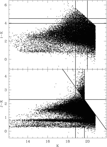
The colour–magnitude diagrams for EROs (top panel) and DRGs (bottom panel). The lines indicate the selection criteria for each population. For display purpose, only 20 per cent of all detected objects for iK and JK diagrams are displayed. The open circles are DRG candidates having J > 22.
Fig. 5 shows the number counts of EROs (top panel) and DRGs (bottom panel). The upper lines in each panel are number counts of all galaxies. In the top panel of Fig. 5, results from the UKIDSS UDS (asterisk, Lane et al. 2007), Deep3a-F (filled triangle) and Daddi-F (filled square) from Kong et al. (2006) and EROs with R −K > 5.3 and 6 (open square and triangle) from Simpson et al. (2006) were also plotted for comparison. The number counts of all galaxies in SA22 field are in agreement with previous results. However, all galaxies with matching i and K detections (top) show slightly lower density at faint magnitudes, since our i depth is not sufficient to cover the full near-IR depth. Similarly, our ERO counts are slightly below those from previous results because of our relative depth in i. The filled and open circles indicate EROs in SA22 selected by i −K > 4.5 and i −K > 3.96, respectively. The filled triangle and square are results for EROs selected by R −K > 5 from Deep3a-F and Daddi-F of Kong et al. (2006), and the open square and triangle are results for R −K > 5.3 and R −K > 6 EROs from the UKIDSS UDS in Simpson et al. (2006). Our i −K > 3.96 ERO counts are comparable to those of R −K > 5–5.3 EROs and our i −K > 4.5 ERO counts match those of R −K > 6 EROs. See Section 5.4 for a discussion of how the colour selection affects the clustering.
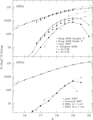
Number counts of all galaxies (upper lines in each panel), EROs (top panel) and DRGs (bottom panel). The top panel shows the number counts of Deep3a-F (filled triangle) and Daddi-F (filled square) in Kong et al. (2006), R −K > 5.3 (open square) and R −K > 6.0 (open triangle) EROs in Simpson et al. (2006), all galaxies (asterisk) in Lane et al. (2007) and this work (star). The results of two selection criteria are presented by the open circle (i −K > 3.96) and filled circle (i −K > 4.5) symbols. The bottom panel shows all galaxies (asterisk) in Lane et al. (2007), DRGs (triangle) in Foucaud et al. (2007) and DRGs with a J magnitude cut (black filled circle) and without a J magnitude cut (black open circle); see text for details. Those of all galaxies in this work are results from iK-matched (top panel) and only K (bottom panel) samples.
The bottom panel of Fig. 5 shows the number counts of DRGs. The results for all galaxies with a joint detection of J and K (stars) are in agreement with Lane et al. (2007). In addition, the counts of DRGs are also the same as those of the UKIDSS UDS EDR in Foucaud et al. (2007). We also plot the number counts of DRGs irrespective of whether there is a matched detection in J (open circles), which only shows a significant difference for the faintest bin.
Table 1 lists the number counts of each population. We note that the number counts of all galaxies are from only the K band of the UKIDSS DXS catalogue without a J limit. However, those for EROs and DRGs are limited by the i and J bands, especially at faint magnitudes.
The number counts in log[N(deg−2 0.5 mag−1)] of galaxies, i −K > 3.96 and i −K > 4.5 EROs and DRGs. The number counts of all galaxies are measured using only the K magnitude from the UKIDSS DXS catalogue without a J limit, but those for the EROs and DRGs are limited by the i and J depths.
| K bin | Galaxies | i −K > 3.96 EROs | i −K > 4.5 EROs | DRGs |
| 15.0 | 2.165 | – | – | – |
| 15.5 | 2.465 | – | – | – |
| 16.0 | 2.742 | – | – | – |
| 16.5 | 2.973 | 0.652 | 0.213 | 0.416 |
| 17.0 | 3.174 | 1.690 | 0.991 | 0.814 |
| 17.5 | 3.393 | 2.333 | 1.725 | 1.185 |
| 18.0 | 3.586 | 2.815 | 2.374 | 1.761 |
| 18.5 | 3.759 | 3.092 | 2.747 | 2.306 |
| 19.0 | 3.900 | 3.203 | 2.875 | 2.665 |
| 19.5 | 4.017 | 3.146 | 2.716 | 2.561 |
| 20.0 | 4.101 | 2.678 | 1.815 | – |
4.2 Clustering of EROs
Fig. 6 shows the angular two-point correlation function corrected for the integral constraint of all (top panel), K < 18.8 (middle panel) and K > 18.8 (bottom panel) EROs. Many studies have found that EROs are strongly clustered (Roche et al. 2002, 2003; Brown et al. 2005; Kong et al. 2006, 2009). A power-law fit to the angular correlation function is consistent with the previous data with no significant differences in the measured slope. However, all of these studies have been restricted to relatively narrow fields (<20 arcmin on a side) and small samples (<500 galaxies). In this study, we represent the correlation function of EROs on much wider scales and with a larger sample than before. We confirm that EROs are strongly clustered at all of the angular scales sampled. There is an apparent inflection at θ∼ 0.6–1.2 arcmin, implying that a double power law is required to fit the correlation function of EROs. This has been observed for LRGs (Ross et al. 2008; Sawangwit et al. 2010) and DRGs at 2 < z < 3 (Quadri et al. 2008) and is naturally explained by the one- and two-halo terms arising in the halo model of galaxy clustering. We fit the correlation function of EROs by separating small (θ < 0.76 arcmin) and large (0.76 < θ < 19 arcmin) scales and apply these ranges for all other ERO samples. The slopes of each power law were measured from K < 18.8 and i −K > 4.5 ERO samples by the fit described in Section 3.4, and then those were applied to all K > 18.8 EROs, since our i-band magnitude limit prevents a complete extraction of the faint EROs. The measured slopes are 0.99 ± 0.09 for the small scales and 0.40 ± 0.03 for the larger scales. The slopes are slightly smaller than those for LRGs at z < 1 (1.16 ± 0.07 and 0.67 ± 0.07 of 2SLAQ and 1.28 ± 0.04 and 0.58 ± 0.09 of AAΩ for small and large scale, respectively) in Ross et al. (2008). However, our values are in agreement with DRGs at 2 < z < 3 (1.2 ± 0.3 and 0.47 ± 0.14 for small and large scale respectively) in Quadri et al. (2008) within the uncertainty ranges. Also bright EROs show a larger amplitude than others, that is, stronger clustering. The second and third columns in Table 2 list the amplitudes measured.
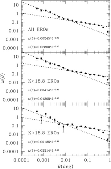
The integral constraint corrected angular two-point correlation functions of all (top panel), K < 18.8 (middle panel) and K > 18.8 (bottom panel) EROs. The dotted lines and equations in each panel show power-law (Aωθ−δ) fitting results at small and large scale.
The amplitudes Aω of the correlation functions and the number of selected objects in the ERO and DRG samples.
| Criterion | Asmallω(×10−3) | EROs Alargeω(×10−3) | Number | Asmallω(×10−3) | DRGs Alargeω(×10−3) | Number |
| All | 2.45 ± 0.13 | 28.00 ± 0.39 | 5383 | 0.19 ± 0.02 | 7.30 ± 0.44 | 3414 |
| K < 18.8 | 4.14 ± 0.33 | 42.05 ± 0.93 | 2277 | 0.37 ± 0.10 | 23.63 ± 1.57 | 979 |
| K > 18.8 | 1.35 ± 0.20 | 22.14 ± 0.67 | 3106 | 0.16 ± 0.03 | 6.23 ± 0.67 | 2435 |
Perhaps the most striking result is the very shallow slope of the clustering on the larger scales. The value of 0.4–0.5 is in stark contrast to the canonical value of 0.8 that is so widely found in lower redshift studies and assumed for more distant studies when the slope is poorly constrained. For our ERO and DRG samples, the DRGs in Quadri et al. (2008) and the FIR-selected galaxies in Cooray et al. (2010), the strongly clustered objects are being compared in projection over a range of the order of unity in redshift and all show relatively shallow slopes on scales equivalent to 5–50 h−1 Mpc. This contrasts with the equivalent angular clustering of LRGs by Sawangwit et al. (2010), where the depth in redshift is at most 0.2 and the slope is steeper. A similar change in the slope has been noted in faint galaxy clustering by Neuschaefer & Windhorst (1995) and Postman et al. (1998) in which they parametrized the change in slope as δ(z) = 1.75–1.8(1 +z)−0.2−0.35− 1, where z is the median redshift of the galaxies sampled. This functional form is consistent with the shallower slope we find for EROs compared to LRGs as long as the index is less than −0.3, although this would predict a much shallower slope at higher redshifts which would appear to be inconsistent with results.
The origin of this change in slope in the angular clustering is a combination several factors. The primary one is the fact that the angular diameter distance at redshifts above 0.8 is relatively constant, although this is strongly dependent on the cosmological parameters as shown by Kauffmann et al. (1999) from N-body simulations. Indeed, the angular clustering as a function of redshift may be a relatively simple test of the cosmological constant and has been proposed as a method to detect the baryon accoustic oscillation scale by Sánchez et al. (2010). Another effect that leads to the flattening of the slope may also be the redshift range sampled as the clustering is diluted as galaxies of differing distances are compared. We note that Sánchez et al. (2010) predict a significantly shallower slope for the angular clustering as the redshift range increases on the scales we are considering here. Future studies will be able to test this directly with improved photometric redshift accuracy.
Our results need to be compared to previous results with careful attention to the differences in our selection and measurement. Thus, we applied the same method as applied in the previous studies, which measured the integral constraint and the amplitude of the correlation function by a single power law with the fixed slope as δ = 0.8. First, we consider the amplitude of the clustering, which may appear to differ only because of the fact that we are fitting a double power law. Fitting a single power law to the angular clustering of K < 18.8 and i −K > 4.5 EROs, we measure an amplitude of (12.72 ± 0.5) × 10−3, which is consistent with (14.60 ± 1.64) × 10−3 of Daddi-F EROs at the same magnitude limit, but slightly larger than (9.29 ± 1.60) × 10−3 of Deep3a-F EROs in Kong et al. (2006). In addition, our value is larger than (6.6 ± 1.1) × 10−3 of Kong et al. (2009). However, this difference may be the result of the different selection criteria and angular ranges used. To illustrate this, if we fit over the angular range sampled by Kong et al. (2009) of 0.19 and 3 arcmin to measure the amplitude of i −K > 3.96 and K < 18.8 EROs with a single power law with δ = 0.8, then we recover a value of (6.65 ± 0.3) × 10−3 that does match their published value. Therefore, our results are entirely consistent with Kong et al. (2009), given the effects of cosmic variance (see Section 5.6), even though the slopes and amplitudes we quote appear to differ on first inspection.
Secondly, if a single power law is applied to fit the correlation function, the reduced χ2 value is 2.8. However, the value drops to 0.3 for small scales and 1.5 for large scales, when the double power law with the measured slopes is applied. Thus, a double power law well describes the correlation function of our EROs, but past observations have not uncovered it due to their limited angular sampling and larger errors.
The clustering properties as a function of the limiting magnitude and colour are discussed in Section 5.
4.3 Clustering of DRGs
Applying a similar analysis to the angular clustering of DRGs, we again find that a double power-law fit is required (Fig. 7). While most early attempts to measure the angular correlation of DRGs were consistent with a single power law (Grazian et al. 2006; Foucaud et al. 2007), Quadri et al. (2008) demonstrated that a double power law with an inflection at θ∼ 0.17 arcmin was appropriate to fit the angular correlation function of 2 < z < 3 DRGs in the UKIDSS UDS field. However, the angular ranges for the small and large scales used in their fitting were split at 0.67 arcmin. To ensure that our results can be compared, we have used the power-law slope for the large-scale clustering found by Quadri et al. (2008), δ = 0.47, and measured that for the small scales from a free fit to δ after the integral constraint correction.
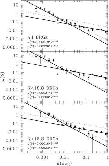
The angular two-point correlation functions corrected for the integral constraint of all (top panel), K < 18.8 (middle panel) and K > 18.8 (bottom panel) DRGs. The solid lines and equations in each panel show power-law fitting results. The dotted lines are the best-fitting results for 2 < z < 3 DRGs from Quadri et al. (2008).
In order to measure an amplitude and slope for each angular range, small and large scales were split at 0.48 arcmin, since our correlation functions showed an upturn at θ < 0.48 arcmin. The power-law slope for small scales was then measured for K < 18.8 DRGs, which is not affected by the J magnitude limit. The measured slope was δ = 1.38 ± 0.27, which is consistent with the value of 1.2 ± 0.3 derived by Quadri et al. (2008), considering the additional photometric redshift constraint they applied.
To directly compare our angular correlation function of DRGs with that in Foucaud et al. (2007), the function for K < 18.8 DRGs was fitted with a single power law with a fixed δ of 1.0 between 0.5 and 12 arcmin to match their magnitude limit and fit constraints. The amplitude of K < 18.8 DRGs, (3.07 ± 0.6) × 10−3, is consistent with 3.1+2.1−1.3× 10⁻³ in Foucaud et al. (2007).
Fig. 7 presents the angular correlation functions corrected for the integral constraint for all (top panel), K < 18.8 (middle panel) and 18.8 < K < 19.7 (bottom panel) DRGs with fitted power laws. The solid and dotted lines are the fitted power law and that for 2 < z < 3 DRGs in Quadri et al. (2008), respectively. It is apparent that DRGs are strongly clustered, and their correlation functions are well described by a double power law. There are clear differences in the amplitude of clustering on both small and large scales between our brighter and fainter DRGs and in the angular scale for the inflection compared to the Quadri et al. (2008) sample. The measured amplitudes are listed in Table 2 but should be used with care, given the complex interplay between the depth, redshift sampled and angular coverage of DRG samples.
5 DISCUSSION
5.1 Magnitude-limited EROs
It is well known that the clustering of EROs depends on the limiting magnitude of any selection criterion (Daddi et al. 2000; Roche et al. 2002, 2003; Brown et al. 2005; Georgakakis et al. 2005; Kong et al. 2006, 2009). However, in previous cases, a single power law was invoked to describe the angular correlation function. In this section, we discuss the clustering properties at small and large scales with various magnitude limits to expand on these previous studies.
To select EROs at each magnitude limit, the colour was fixed at i −K > 4.5. We applied the same slopes of power law and fitting ranges as used in Section 4.2 for small and large scales, and fitted ω(θ) =Aωθ−δ to the correlation function. Fig. 8 shows the angular two-point correlation functions corrected for the integral constraint and fitted results for various subsets of EROs using different limiting magnitudes with a fixed colour. It is apparent that a double power law is required to fit the correlation function of EROs for all magnitude limits.
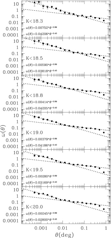
The angular two-point correlation functions corrected for the integral constraint and fitted power laws for various magnitude-limited samples of EROs.
The top panel in Fig. 9 shows the amplitude of each power law with fixed slopes as a function of the limiting magnitude (filled symbols). Although faint EROs may not be complete because of the relatively shallow i depth, there is a trend in the amplitude at the brightest limiting magnitudes. The amplitude of the small scale varies significantly. However, the amplitude of the large scale shows an almost constant value at all magnitude limits.
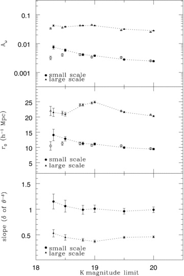
The amplitudes (top panel) and real-space correlation lengths (middle panel) of double power-law fits with fixed slopes (δ = 0.99, 0.40) for magnitude-limited EROs and the measured slope (bottom panel) as a function of the limiting magnitude. The open symbols in the top and middle panels are results when the slope is allowed to vary. Those are slightly shifted for display purposes.
The variation in amplitude at small scales is also apparent in the real-space correlation length in the middle panel of Fig. 9 (filled symbols). As mentioned in Section 3.4, the amplitudes measured with fixed slopes from i −K > 4.5 and K < 18.8 EROs were used to calculate the correlation length. The correlation length for the small scales shows a range between 9 and 14 h−1 Mpc with the strongest clustering for the brighter galaxies. On the other hand, the clustering on large scales shows a similar length of 21–24 h−1 Mpc that varies marginally over the range in magnitude sampled.
To investigate the variation in slope, we measured slopes by fitting a power law with a free slope. The results are presented in the bottom panel of Fig. 9. The slope of the brighter subsamples have higher values than the fainter ones, that is, brighter EROs show steeper correlation functions especially on small scales. The amplitudes and correlation lengths from freely fitted slopes are presented in the top and middle panels of Fig. 9 with the open symbols. For display purposes, the points are slightly shifted in magnitude. All estimated values with fixed slopes are listed in Table 3 and those with variable slopes are listed in Table 4.
The amplitudes Aω of the correlation functions, correlation lengths with fixed slopes and number of EROs for each magnitude limit.
| K limit | Asmallω(×10−3) | Alargeω(×10−3) | rsmall0(h−1 Mpc) | rlarge0(h−1 Mpc) | χ2small,large | Number |
| K < 18.3 | 7.52 ± 1.1 | 42.06 ± 2.5 | 14.09 ± 1.9 | 21.51 ± 1.3 | 0.9, 2.1 | 852 |
| K < 18.5 | 5.90 ± 0.6 | 38.18 ± 1.6 | 12.85 ± 0.7 | 20.92 ± 0.6 | 0.3, 2.8 | 1323 |
| K < 18.8 | 4.14 ± 0.3 | 42.05 ± 0.9 | 11.29 ± 0.5 | 23.97 ± 0.4 | 0.3, 1.5 | 2277 |
| K < 19.0 | 3.79 ± 0.3 | 41.86 ± 0.7 | 11.12 ± 0.4 | 24.89 ± 0.3 | 3.2, 2.0 | 3014 |
| K < 19.5 | 2.80 ± 0.2 | 31.69 ± 0.5 | 9.96 ± 0.3 | 21.60 ± 0.2 | 2.0, 3.1 | 4713 |
| K < 20.0 | 2.45 ± 0.1 | 28.00 ± 0.4 | 9.48 ± 0.3 | 20.29 ± 0.2 | 1.9, 3.6 | 5383 |
The amplitudes Aω of the correlation functions, correlation lengths with variable slopes and estimated variable slopes of EROs for each magnitude limit.
| K limit | Asmallω(×10−3) | Alargeω(×10−3) | rsmall0(h−1 Mpc) | rlarge0(h−1 Mpc) | Slopesmall | Slopelarge | χ2small,large |
| K < 18.3 | 3.20 ± 0.4 | 33.26 ± 1.9 | 10.51 ± 1.4 | 21.97 ± 1.5 | 1.15 ± 0.15 | 0.53 ± 0.07 | 0.7, 1.8 |
| K < 18.5 | 4.05 ± 0.4 | 34.92 ± 1.5 | 11.28 ± 0.6 | 21.27 ± 0.6 | 1.06 ± 0.12 | 0.45 ± 0.05 | 0.2, 2.7 |
| K < 18.8 | 4.14 ± 0.3 | 42.05 ± 0.9 | 11.29 ± 0.5 | 23.97 ± 0.4 | 0.99 ± 0.09 | 0.40 ± 0.03 | 0.3, 1.5 |
| K < 19.0 | 3.40 ± 0.2 | 44.14 ± 0.8 | 10.71 ± 0.4 | 24.59 ± 0.3 | 1.01 ± 0.07 | 0.37 ± 0.02 | 0.4, 1.8 |
| K < 19.5 | 3.31 ± 0.2 | 28.98 ± 0.4 | 10.54 ± 0.3 | 21.94 ± 0.2 | 0.96 ± 0.06 | 0.45 ± 0.02 | 2.0, 2.1 |
| K < 20.0 | 2.45 ± 0.1 | 25.14 ± 0.4 | 9.60 ± 0.3 | 20.70 ± 0.2 | 0.99 ± 0.05 | 0.46 ± 0.02 | 1.9, 2.3 |
To compare with previous results, we again need to fit a single power law to a smaller range in angle. We find that the correlation length of K < 20 and i −K > 4.5 EROs with a fixed δ = 0.8 is 16.99 ± 0.2 h−1 Mpc, which is consistent with 12–17 h−1 Mpc found in Georgakakis et al. (2005). Our value may be higher than the value of Georgakakis et al. due to our redder colour limit that preferentially selects more massive galaxies. Furthermore, the correlation length of our K < 18.8 and i −K > 3.96 EROs fitted by a single power law (see Section 4.2) is 12.52 ± 0.33 h−1 Mpc, which is higher than 9.6 ± 0.1 or 9.2 ± 0.2 h−1 Mpc in Kong et al. (2009), although the amplitudes are all consistent. This is most probably caused by the different redshift distributions of the Kong R −K sample. Applying the different criteria to the NMBS sample, our selection has a slightly larger fraction of galaxies at 1.5 < z < 2.0 than that in Kong et al. (2009).
5.2 Colour-limited EROs
Daddi et al. (2000) studied the clustering amplitude as a function of the colour threshold. They pointed out that red galaxies have a higher amplitude, but the amplitudes of R −K > 5.0 and R −K > 5.3 EROs were consistent. In addition, Brown et al. (2005) also noted no significant difference in amplitude of R −K > 5.0 and 5.5 EROs. However, the small area or shallower depth of previous studies may have prevented a sufficiently accurate measurement of the ERO clustering to recover these differences. In this section, we discuss the clustering properties of EROs as a function of the colour limit using wider coverage than Daddi et al. (2000) and deeper imaging than Brown et al. (2005).
We used only K < 18.8 ERO samples with various colour limits, since the i depth is too shallow to cover the full near-IR depth for the reddest subsamples. Fig. 10 shows angular correlation functions corrected for the integral constraint for various colour limits and the fitted power laws. The same ranges and fixed slopes from Section 4.2 were applied to fit the functions. As verified in previous sections, the double power law well describes the functions of all colour-limited EROs. However, the correlation functions show different trends from those of magnitude-limited EROs. The relation between the amplitude and colour limit is presented in the top panel of Fig. 11 (filled symbols). It is clear that redder EROs have higher amplitudes, that is, stronger clustering. Moreover, there is a similar trend in the amplitude as a function of colour limit for both small and large scales. This is also evident in the trend of the real-space correlation length in the middle panel of Fig. 11 (filled symbols), but the correlation lengths for large scales vary most dramatically. This increased clustering with colour limit is entirely as expected, given the correlation between the colour and lower redshift limit of the selection. The redder colour cuts select more distant, more luminous galaxies that are therefore more clustered. In the bottom panel of Fig. 11, the slopes measured independently show similar values for each scale at all colour limits. The lack of any variation with colour indicates that the form of the clustering does not change dramatically with redshift. The values of the freely fitted slope are also marked as the open symbols in the top and middle panels in Fig. 11. The measured values using a fixed slope are listed in Table 5 and those with a variable slope are listed in Table 6.
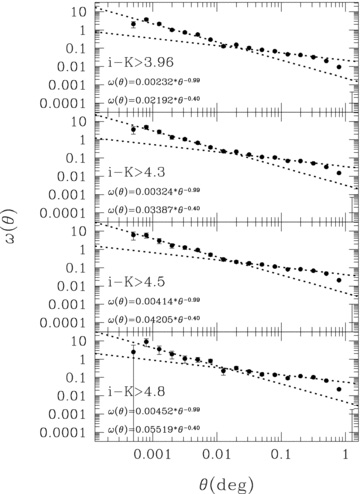
The angular two-point correlation functions corrected for the integral constraint and fitted results for various colour limits.
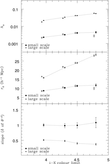
The amplitudes (top panel) and real-space correlation lengths (middle panel) of double power-law fits with fixed slopes (δ = 0.99, 0.40) for colour-limited EROs and measured slope (bottom panel) as a function of colour limits. The open symbols in the top and middle panels are measured from fits with a varying slope. Those are slightly shifted for display purposes.
The amplitudes Aω of the correlation functions, the correlation lengths with fixed slopes and the number of EROs for each colour limit.
| i −K limit | Asmallω(×10−3) | Alargeω(×10−3) | rsmall0(h−1 Mpc) | rlarge0(h−1 Mpc) | χ2small,large | Number |
| i −K > 3.96 | 2.32 ± 0.1 | 21.92 ± 0.4 | 8.63 ± 0.2 | 15.75 ± 0.2 | 3.2, 5.6 | 5654 |
| i −K > 4.3 | 3.24 ± 0.2 | 33.87 ± 0.6 | 10.24 ± 0.4 | 21.39 ± 0.3 | 0.6, 3.7 | 3313 |
| i −K > 4.5 | 4.14 ± 0.3 | 42.05 ± 0.9 | 11.29 ± 0.5 | 23.97 ± 0.4 | 0.3, 1.5 | 2277 |
| i −K > 4.8 | 4.52 ± 0.6 | 55.19 ± 1.4 | 11.66 ± 0.9 | 28.48 ± 0.5 | 0.8, 5.0 | 1259 |
The amplitudes Aω of the correlation functions, the correlation lengths with variable slopes and the estimated slopes of EROs for each colour limit.
| i −K limit | Asmallω(×10−3) | Alargeω(×10−3) | rsmall0(h−1 Mpc) | rlarge0(h−1 Mpc) | Slopesmall | Slopelarge | χ2small,large |
| i −K > 3.96 | 2.19 ± 0.1 | 17.95 ± 0.3 | 8.46 ± 0.2 | 16.41 ± 0.2 | 1.00 ± 0.05 | 0.51 ± 0.02 | 3.2, 2.2 |
| i −K > 4.3 | 3.43 ± 0.2 | 29.32 ± 0.6 | 10.45 ± 0.4 | 21.81 ± 0.3 | 0.98 ± 0.07 | 0.48 ± 0.02 | 0.6, 2.3 |
| i −K > 4.5 | 4.14 ± 0.3 | 42.05 ± 0.9 | 11.29 ± 0.5 | 23.97 ± 0.4 | 0.99 ± 0.09 | 0.40 ± 0.03 | 0.3, 1.5 |
| i −K > 4.8 | 2.79 ± 0.4 | 57.52 ± 1.4 | 9.92 ± 0.7 | 27.97 ± 0.5 | 1.08 ± 0.17 | 0.37 ± 0.03 | 0.8, 4.8 |
5.3 Populations of EROs
The simple colour selection of EROs, while effective and easy to implement, does not necessarily return a uniform population of galaxies. It is known that EROs can be classified into old passively evolved galaxies (OGs) and dusty star-forming galaxies (DGs). Pozzetti & Mannucci (2000) suggested a colour criterion in the (I −K) versus (J −K) plane defined by differences in the SEDs for old stellar populations and dusty galaxies. However, in this study, the i filter was used instead of I. Therefore, we adopted the criterion, (J −K) = 0.20(i −K) + 1.08, defined in the (i −K) versus (J −K) plane by Fang, Kong & Wang (2009). Fig. 12 shows the two-colour diagram of K < 18.8 EROs for classifying OGs and DGs. The line indicates the criterion defined by Fang et al. (2009). The fraction of OGs with K < 18.8 and i −K > 4.5 is ∼63 per cent. This value is consistent with the fractions found for K < 19.7 EROs selected by I −K and R −K in Conselice et al. (2008). The fractions of DGs selected by various magnitude cuts with i −K > 4.5 are 36 per cent at K < 18.5 and 41 per cent at K < 20, although this may be affected by the shallow i-band depth. The fraction of colour-limited K < 18.8 DGs are 43 per cent for i −K > 3.96 EROs and 36 per cent for i −K > 4.8 EROs.
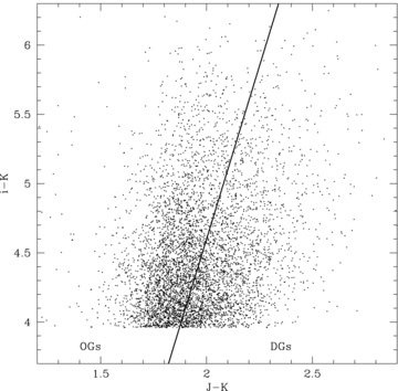
The i −K versus J −K colour–colour diagram for K < 18.8 EROs. The line indicates the criterion defined by Fang et al. (2009) to classify OGs and DGs.
Fig. 13 shows the angular correlation functions corrected for the integral constraint of OGs (left-hand panel) and DGs (right-hand panel). In addition, correlation functions were measured with various colour (top panel) and magnitude (bottom panel) limits. The dotted line of each panel indicates the best fit for the correlation function for K < 18.8 and i −K > 4.5 EROs. Since the small number of objects for i −K > 4.8 DGs can cause a poor statistical and uncertain integral constraint, i −K > 4.8 DGs were excluded for analysis. The most apparent features are that the correlation functions for OGs show a clear break at the same position as that for all EROs in Section 4.2, and OGs are more clustered than the full ERO sample as a function of both the magnitude and colour limit, especially on large scales. Conversely, the correlation functions of DGs show much more scatter between subsamples in magnitude and colour and are much less clustered than OGs and the full ERO sample. This can be attributed to their wider redshift range and lower intrinsic mass.
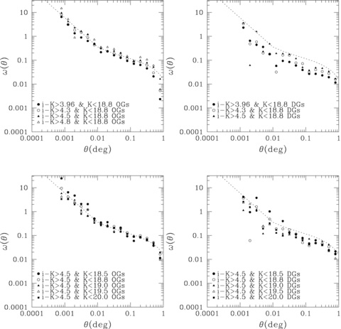
The angular correlation functions corrected for the integral constraint of OGs (left-hand side) and DGs (right-hand side). Also shown are the correlation functions for magnitude-limited (bottom panel) and colour-limited (top panel) samples. The dotted line indicates the best fit for the correlation function of K < 18.8 and i −K > 4.5 EROs.
These trends are also confirmed in the real-space correlation lengths in Fig. 14. Fig. 14 shows the correlation length of OGs (filled symbols) and DGs (open symbols) on small (circle) and large (triangle) scales plotted for various magnitude (bottom) and colour (top) limits. As the angular correlation function of some DG samples was not measured at ∼0.05 arcmin, to estimate the correlation length, the range between 0.076 and 0.76 arcmin for small scales (i.e. narrower than that used earlier) was fitted with the fixed slopes used in Section 4.2. This may lead to slightly different correlation lengths at small scales, but it should not affect any overall trends. The most important feature of the correlation lengths is the trend within each population. The magnitude-limited OGs show no significant change in clustering on large scales and only a weak decline in small-scale clustering strength, as the uniformity of the correlation functions in Fig. 13 implies. However, redder OGs have larger correlation lengths than bluer ones, since redder OGs are more distant and more massive galaxies. Indeed, the similarity in the clustering in strength and functional form to that of low-redshift LRGs in Sawangwit et al. (2010) implies that there is a continuity in the selection of massive, passive galaxies that can be made from optical and near-IR surveys. Similarly, the DGs show more significant variation in clustering with the colour and magnitude.
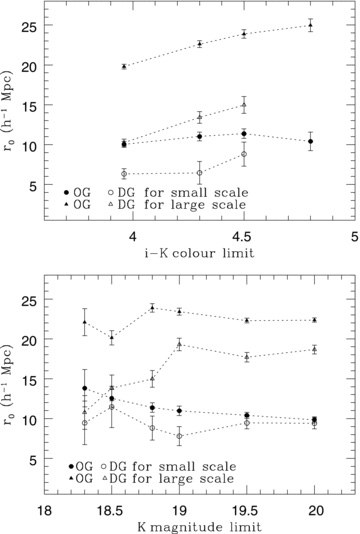
The correlation length of OGs (filled symbols) and DGs (open symbols) for various magnitude (bottom panel) and colour (top panel) limits.
The consistency in clustering within the OG and DG samples contrasts with the much more significant changes in clustering seen in Figs 9 and 11. These trends can be attributed to the changes in the relative proportion of OGs and DGs as a function of the colour and magnitude. For instance, the decreased clustering on large scales for the brightest and bluest EROs coincides with the largest fraction of DGs (up to 43 per cent) resulting in lower clustering strength. These results highlight the need to treat the selection of EROs with care as the diversity of galaxies selected can lead to misleading clustering trends.
5.4 EROs selected by r −K colour
Although various colour selection criteria have been used in previous studies to select EROs, the differences between the criteria have not been well characterized. In this section, we briefly compare the clustering of EROs selected by r −K and i −K colours to attempt to clarify how the use of a different optical filter affects their statistical and clustering properties.
Fig. 15 shows the observed angular correlation functions of 5564 K < 18.8 EROs, which are selected by i −K > 3.96 (filled circle), 4326 EROs by r −K > 5 and r < 24 (the peak of our r-band number counts) (open circle), 7185 EROs by r −K > 5 without r magnitude cut (filled triangle) and 4799 EROs by r −K > 5.3 without an r-magnitude cut (open triangle). It is clear that r −K > 5.3 EROs are more clustered than r −K > 5 EROs, matching the results found with i −K selection. However, the most apparent feature is that each sample shows different clustering properties, particularly on larger scales. The EROs selected by i −K > 3.96 show the highest amplitude of all the samples and the slope of the clustering on larger scales varies significantly with colour. These different clustering properties are most easily explained by the changes in the redshift distribution between samples and the different proportion of OGs to DGs. Conselice et al. (2008) mentioned that the I −K > 4 criterion is more useful to select EROs at higher redshift than r −K > 5.3. In fact, r-band magnitudes of half of our i −K > 3.96 EROs are fainter than our r = 24 magnitude limit, so any r −K sample would be incomplete. Conversely, 27 per cent of the EROs selected by r −K > 5 without an r cut from our sample have i −K < 3.96 and would hence not have been considered in any of our i −K samples. The r −K > 5 EROs that are blue in i −K will be at lower redshifts, lower mass and therefore less clustered.
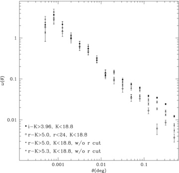
The observed angular correlation functions of K < 18.8 EROs with i −K > 3.96 (filled circle), r −K > 5 and r < 24 (open circle), r −K > 5 without an r cut (filled triangle) and r −K > 5.3 without an r cut (open triangle). It is noted that an integral constraint correction has not been applied to these functions.
5.5 Clustering of EROs and DRGs
The goal of the colour criteria for EROs and DRGs is to select red galaxies that are likely to be at high redshift (z > 1 or z > 2). However, Lane et al. (2007) and Quadri et al. (2007) found that the colour cut for DRGs can include a significant fraction of relatively low redshift objects (0.8 < z < 1.4) that are dust obscured. In this section, we briefly discuss the comparison of two different populations with clustering properties.
Table 7 lists correlation lengths of i −K > 4.5 EROs and J −K > 2.3 DRGs. It is apparent that brighter samples show stronger clustering. Although the direct comparison of correlation length is difficult because of different slopes and redshift distributions, we can confirm that EROs are more clustered than DRGs from the comparison of Figs 6 and 7, and correlation lengths. This was also found by Foucaud et al. (2007).
The correlation length r0 (h−1 Mpc) of selected objects for EROs and DRGs.
| Criterion |  |  |  |  |
| All | 9.48 ± 0.3 | 20.29 ± 0.2 | 4.66 ± 0.2 | 10.32 ± 0.4 |
| K < 18.8 | 11.29 ± 0.5 | 23.97 ± 0.4 | 5.14 ± 0.6 | 17.19 ± 0.8 |
| K > 18.8 | 7.12 ± 0.6 | 17.45 ± 0.4 | 4.42 ± 0.4 | 9.52 ± 0.7 |
| Criterion | | | | |
| All | 9.48 ± 0.3 | 20.29 ± 0.2 | 4.66 ± 0.2 | 10.32 ± 0.4 |
| K < 18.8 | 11.29 ± 0.5 | 23.97 ± 0.4 | 5.14 ± 0.6 | 17.19 ± 0.8 |
| K > 18.8 | 7.12 ± 0.6 | 17.45 ± 0.4 | 4.42 ± 0.4 | 9.52 ± 0.7 |
The correlation length r0 (h−1 Mpc) of selected objects for EROs and DRGs.
| Criterion | | | | |
| All | 9.48 ± 0.3 | 20.29 ± 0.2 | 4.66 ± 0.2 | 10.32 ± 0.4 |
| K < 18.8 | 11.29 ± 0.5 | 23.97 ± 0.4 | 5.14 ± 0.6 | 17.19 ± 0.8 |
| K > 18.8 | 7.12 ± 0.6 | 17.45 ± 0.4 | 4.42 ± 0.4 | 9.52 ± 0.7 |
| Criterion | | | | |
| All | 9.48 ± 0.3 | 20.29 ± 0.2 | 4.66 ± 0.2 | 10.32 ± 0.4 |
| K < 18.8 | 11.29 ± 0.5 | 23.97 ± 0.4 | 5.14 ± 0.6 | 17.19 ± 0.8 |
| K > 18.8 | 7.12 ± 0.6 | 17.45 ± 0.4 | 4.42 ± 0.4 | 9.52 ± 0.7 |
However, it has been shown that the J −K > 2.3 criterion selects 1 < z < 2 objects as well as ones at z > 2 (Grazian et al. 2006; Papovich et al. 2006; Conselice et al. 2007; Lane et al. 2007). Quadri et al. (2007) also pointed out that the fraction of z < 1.8 DRGs is 15 per cent at K < 21 and 50 per cent at K < 19. Therefore, from the different clustering properties of the two populations, we can contrast them at 1 < z < 2, where most bright DRGs and i −K > 4.5 EROs are located. The different clustering properties in the bin indicate that EROs and DRGs may have different characteristics. In fact, Conselice et al. (2007) demonstrated that 1 < z < 2 DRGs show a broad range in stellar mass and that EROs are more massive than DRGs at the same redshift (Conselice et al. 2008). These mass differences can explain the stronger clustering of EROs compared to bright DRGs, since massive objects are expected to be more clustered. Furthermore, contamination from low-redshift DRGs may lead to the variation of clustering between our samples and 2 < z < 3 DRGs seen in Fig. 7. The fraction of z < 1.6 DRGs at K > 18.8 magnitude range is ∼40 per cent in NMBS redshift distribution. This effect is also verified by the weaker clustering of r −K EROs in the previous section. This means that when using a simple colour criterion it is difficult to avoid a contribution from different types of galaxy or galaxies over a wide range in redshift.
Our correlation lengths of DRGs are apparently different from previous results. If a single power law is applied for our K < 18.8 DRGs, the correlation length is 9.5 ± 1.0 h−1 Mpc. This value is smaller than 14.1+4.8−2.9h−1 Mpc with σ = 0.5 redshift distribution or 11.1+3.8−2.3h−1 Mpc using a Gaussian redshift distribution with z = 1 and σ = 0.25 in Foucaud et al. (2007) but is within the error range of both these estimates. These apparent differences may be caused by differences in the redshift distribution. The NMBS redshift distribution is broader and more complicated than that assumed in Foucaud et al. and is likely to better reflect the true DRG redshift distribution. Quadri et al. (2008) measured r0 = 10.6 ± 1.6 h−1 Mpc on a large scale for 2 < z < 3 DRGs. This is consistent with our results for faint DRGs, but smaller than for our brighter DRGs. The improvement in the photometric redshift measurement for galaxies at z > 1 that the NMBS provides is considerable. Future broad-band studies will benefit from the NMBS constraints on redshift distributions.
5.6 Cosmic variance

The last term gives the correction for Poisson shot noise. Garilli et al. (2008) compared cosmic variances defined by the above equation and correlation functions from the VIMOS VLT Deep Survey (VVDS) data, and argued that the values were in agreement. Therefore, we simply used the above equation to estimate the cosmic variance.
We divided the SA22 field into nine subfields using two criteria, CTIO Blanco field of view (∼0.36 deg2) and WFCAM field of view (∼0.8 deg2), with i −K > 4.5 and K < 18.8 EROs. However, the actual masked average areas were ∼0.27 deg2 and ∼0.63 deg2 for Blanco and WFCAM size fields, respectively. The number density of EROs in each field was calculated and used in equation (8). We note that the field-to-field ratios of number density were consistent with those for various brighter magnitude limits. Therefore, the field-to-field variation at this magnitude range is not a systematic effect, unlike a change in the limiting magnitude or area. The measured cosmic variances were 0.30 and 0.20 for Blanco and WFCAM field size, respectively.
In fact, it is known that the spatial distribution of EROs is inhomogeneous (Daddi et al. 2000; Kong et al. 2006), at least in part due to the strong clustering that EROs exhibit. Fig. 16 shows the spatial distribution of i −K > 4.5 and K < 18.8 EROs. As checked by the number density variation of each subfield and Fig. 16, the distribution of our EROs is also inhomogeneous. There are some overdense regions in the northern part of the field. Moreover, Fig. 17 shows the angular correlation functions corrected for the integral constraint of i −K > 4.5 and K < 18.8 EROs in each subfield by the Blanco size (left-hand panel) and WFCAM size (right-hand panel). The solid lines indicate the best fit of the correlation function for i −K > 4.5 and K < 18.8 EROs in the whole field. It appears that the correlation functions show the most variation on Blanco field size scales. In particular, the standard deviations of the amplitudes of the angular correlation function on large scales are 0.011 and 0.007 for CTIO and WFCAM size subfields, respectively. Also, the standard deviations of the correlation lengths are 4.5 and 2.8 h−1 Mpc, respectively. These results demonstrate that cosmic variance for these field sizes can significantly affect the uncertainty of the measured clustering strength and is likely to have been the dominant source of error in previous clustering analyses of high-redshift galaxies. It is apparent that a large-area survey is important not only to confidently measure number counts, but also to investigate clustering properties.
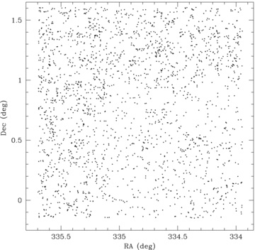
The spatial distribution of K < 18.8 and i −K > 4.5 EROs.
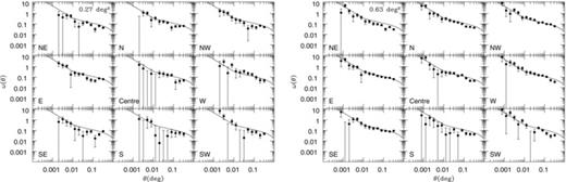
The angular correlation functions corrected for the integral constraint of EROs for 0.27-deg2 (left-hand panel) and 0.63-deg2 (right-hand panel) fields at each position. The solid lines indicate the best fit of K < 18.8 and i −K > 4.5 EROs in the whole field.
6 CONCLUSIONS
We have used near-IR images from the UKIDSS DXS DR5 and gri optical images from the CTIO 4-m Blanco Telescope to investigate the clustering properties of EROs and DRGs in the ∼3.3 deg2 SA22 field. This is the largest area survey of such galaxies to date, and using the precise redshift distributions from the NMBS, we have made the most accurate measurements of the cluster of EROs and DRGs. The results are summarized as follows:
Colour selection criteria were applied to extract EROs and DRGs. In total 5383 EROs with i −K > 4.5, i < 24.6 and K < 20.0 were selected. In addition, 3414 DRGs were extracted by a J −K > 2.3 with J < 22 and K < 19.7 limits. The number density of EROs was well matched to previous studies, once the differences in the selection method were taken into account. Similarly, the number density of DRGs was very well matched with the results from the UKIDSS UDS field.
Both populations showed strong clustering properties. Those of EROs are best described by a double power law with inflection at ∼0.6–1.2 arcmin. Assuming a power law, ω(θ) =Aωθ−δ, (Aω, δ) of K < 18.8 and i −K > 4.5 EROs were (0.00414, 0.99) and (0.04205, 0.40) for small and large scales, respectively.
Additionally, a double power law is required to fit the angular correlation function of DRGs with δ = 1.38 and 0.47 for small and large scale, respectively. Our relatively bright magnitude limit samples are diluted by 1 < z < 2 DRGs, so our clustering shows different trends when compared to deeper samples dominated by 2 < z < 3 DRGs.
The angular two-point correlation function of EROs shows clear trends with different magnitude limits, although those for faint samples may be dominant by relatively blue EROs due to the optical limit. With a fixed power-law slope, the amplitude for small scales decreased at fainter magnitudes, but that for large scales was invariable with magnitude. These trends were also confirmed by the real-space correlation length. On the other hand, with variable slopes, the correlation function at bright limits is steeper than for samples with fainter limits.
The colour-limited correlation function of EROs presents slightly different features from the magnitude-limited function. With a fixed slope, clustering amplitudes and real-space correlation lengths for small and large scales were increased with redder colours. However, slopes were comparable between various colour cuts.
The EROs were classified into OGs and DGs by their i −K versus J −K colours. The correlation functions of magnitude-limited OGs show an apparent break at 0.6–1.2 arcmin and similar amplitude at large scales. The redder ones have stronger clustering. However, the functions for DGs showed much weaker clustering. The relative proportion of OGs and DGs with the colour and magnitude can explain the different trends seen in the clustering of the full sample of EROs.
EROs selected either with r −K or i −K colours show different correlation functions, especially on large scales. The EROs selected by i −K > 3.96 are more clustered than those selected by the r −K selection criteria. This may be caused by the different redshift distribution, since the r −K criterion extracts more low-redshift galaxies than the i −K criterion.
EROs are more clustered than DRGs over the same redshift range (1 < z < 2). This is evidence that the two populations at this redshift are different and EROs are likely to be intrinsically more massive than DRGs.
By dividing the full survey field into subfields of different sizes, we demonstrate that cosmic variance is a significant issue for measurements of the correlation function and is likely to have been the dominant source of error in previous measurements of high-redshift red galaxy clustering.
The results from this analysis illustrate the importance of sampling the widest possible fields in the near-IR in order to recover representative clustering properties of distant galaxies. In the near future, the combination of the UKIDSS and VISTA surveys will cover more than an order of magnitude larger area to comparable depth. Our ability to extract the clustering of EROs in these areas is limited only by the depth of comparable optical imaging. We will be applying the same analysis to the other three DXS fields and making use of the additional Spitzer data that these fields enjoy to refine the selection into narrower photometric redshift slices and fitting these with halo occupation distribution models.
Finally, ERO samples are now of sufficient size to offer direct tests to galaxy formation models in terms of number density and clustering, so future comparisons to semi-analytic simulations will be more powerful (Gonzalez-Perez, in preparation).
Authors thank the referee for comments on improving the presentation and content of this paper. We thank the NMBS team for sharing their photometric redshifts of EROs and DRGs in advance of publication. This work is based on the data from the UKIDSS. We are grateful to the UKIDSS team, the staff in the UKIRT, Cambridge Astronomical Survey Unit and Wide Field Astronomy Unit in Edinburgh. The UKIRT is run by the Joint Astronomy Centre on behalf of the Science and Technology Facilities Council of the UK CTIO and National Optical Astronomy Observatory, managed by the Association of Universities for Research in Astronomy, under contract with the National Science Foundation. J-WK thanks for support from the Korean Government's Overseas Scholarship. We thank U. Sawangwit for providing data.
REFERENCES
