Understanding the shape of the galaxy two-point correlation function at z ≃ 1 in the COSMOS field Free

Abstract

1 INTRODUCTION

Advances in the spectroscopic survey capabilities of 8-m class telescopes have allowed us in the recent years to extend detailed studies of the clustering of galaxies to the z≃ 1 Universe (Coil et al. 2004; Le Fèvre et al. 2005; Coil et al. 2006; Meneux et al. 2006; Pollo et al. 2006; de la Torre et al. 2007; Coil et al. 2008; Meneux et al. 2008; Abbas et al. 2010). The most recent contribution to this endeavour is the COSMOS survey (Scoville et al. 2007), and in particular zCOSMOS, its redshift follow-up with the Visible Multi-Object Spectrograph (VIMOS) at the European Southern Observatory (ESO) Very Large Telescope (VLT; Lilly et al. 2007).

Early angular studies of the COSMOS field (McCracken et al. 2007) and more recent analyses of the first 10 000 zCOSMOS redshifts to I_AB= 22.5 have evidenced significant ‘excess’ clustering in the large-scale shape of the two-point angular and projected correlation function. The redshift information from zCOSMOS, in particular, shows this excess to dominate in the redshift range 0.5 < z < 1 (Meneux et al. 2009). More precisely, the shape of the projected two-point correlation function w_p(r_p) appears to decay much less rapidly than observed at similar redshifts in independent data as the VIMOS VLT Deep Survey (VVDS; Meneux et al. 2008) and with respect to predictions of standard Lambda cold dark matter (ΛCDM) cosmology as incarnated by the Millennium Simulation (De Lucia & Blaizot 2007; Kitzbichler & White 2007). The observed flat shape1 is difficult to reconcile with the theory, unless an unrealistic scale-dependent bias between galaxies and matter is advocated. While plausibly related to the presence of particularly rich large-scale structures dominating the COSMOS volume around z≃ 0.7 (e.g. Guzzo et al. 2007; Meneux et al. 2009), this effect still awaits a quantitative explanation.

In a recent series of papers, Abbas & Sheth (2005, 2006, 2007) have used the Sloan Digital Sky Survey (SDSS; York et al. 2000), together with Halo Occupation Distribution (HOD) models (e.g. Cooray & Sheth 2002) to show how in general the amplitude and shape of the galaxy correlation function depend on the environment in which the galaxies are found. Once a local density is suitably defined over a given scale, galaxies living in overdense regions show a stronger clustering than those in average or underdense environments. This is shown to be a consequence of the direct correlation arising in hierarchical clustering between the mass of the dark matter haloes in which galaxies are embedded and their large-scale environment: the mass function of dark matter haloes is top-heavy in high-density regions, thus in selecting galaxies in these environments we are selecting haloes of higher mass, which are more clustered. The net result is to introduce a scale-dependent bias in the observed correlation function, when this is compared to the expected dark matter clustering (Abbas & Sheth 2006, 2007).

In this paper we investigate whether this effect is at work also at z≃ 0.7 and could explain quantitatively the observed shape of w_p(r_p) in the zCOSMOS data.

2 DATA AND METHODS

2.1 The zCOSMOS 10k-bright sample

zCOSMOS is a large spectroscopic survey performed with VIMOS (Le Fèvre et al. 2003) at the ESO–VLT. The zCOSMOS-bright survey (Lilly et al. 2007) has been designed to follow up spectroscopically the entire 1.7 deg² Hubble Space Telescope COSMOS field (Koekemoer et al. 2007; Scoville et al. 2007) down to I_AB= 22.5. We use in this analysis the first-epoch set of redshifts, usually referred to as the zCOSMOS 10k-bright sample (‘10k sample’, hereafter), including 10 644 galaxies. At this magnitude limit, the survey redshift distribution peaks at z≃ 0.6, with a tail out to z≃ 1.2. We only consider secure redshifts, i.e. confidence classes 4.x, 3.x, 9.3, 9.5, 2.4, 2.5 and 1.5, representing 88 per cent of the full 10k sample (see Lilly et al. 2009 for details) and 20.4 per cent of the complete I_AB < 22.5 magnitude-limited parent sample over the same area. These data are publicly available through the ESO Science Data Archive site.2

2.2 Mock galaxy surveys

In addition to the observed data, in this analysis we also make use of a set of 24 mock realizations of the zCOSMOS survey, constructed combining the Millennium Run N-body simulation,3 with a semi-analytical recipe of galaxy formation (Kitzbichler & White 2007). The Millennium Run is a large dark matter N-body simulation that follows the hierarchical evolution of 2160³ particles between z= 127 and 0 in a cubic volume of 500³h⁻³ Mpc³. It assumes a concordance cosmological ΛCDM model with (Ω_m, Ω_Λ, Ω_b, h, n, σ₈) = (0.25, 0.75, 0.045, 0.73, 1, 0.9). The resolution of the N-body simulation, 8.6 × 10⁸h⁻¹ M_⊙, coupled with the semi-analytical model allows one to resolve with a minimum of 100-particle haloes containing galaxies with a luminosity of 0.1L* (see Springel et al. 2005). Galaxies are generated inside these dark matter haloes using the semi-analytic model of Croton et al. (2006), as improved by De Lucia & Blaizot (2007). This model includes the physical processes and requirements originally introduced by White & Frenk (1991) and refined by Kauffmann & Haehnelt (2000), Springel et al. (2001), De Lucia et al. (2004) and Springel et al. (2005). The 24 mocks are created then ‘observed’ as to reproduce the zCOSMOS selection function (Iovino et al. 2010).

2.3 Local density estimator

To characterize galaxy environment we use the dimensionless density contrast measured by Kovač et al. (2010) around each galaxy in the sample. For each galaxy at a comoving position r we compute the dimensionless 3D density contrast smoothed on a scale ⁠, where ρ(r, R) is the density of galaxies measured on a scale R and is the overall mean density at r. ρ(r, R) is estimated around each galaxy of the sample by counting objects within an aperture (defined either through a top hat of size R or a Gaussian filter with similar dispersion). The reconstructed overdensities are properly corrected for the survey-selection function and edge effects. Kovač et al. (2010) studied different density estimators, corresponding to varying galaxy tracers, filter shapes and smoothing scales. Here we use δ_g as reconstructed with a Gaussian filter with dispersion R= 5 h⁻¹ Mpc. Note that the mass enclosed by such filter is equal to that inside a top-hat filter of size ∼ 7.8 h⁻¹ Mpc. We refer the reader to Kovač et al. (2010) for a full description of the technique.

2.4 Expected probability distribution function of the density contrast

The density contrast distribution can be predicted analytically using some approximations. Empirically, it has been found that the probability distribution function (PDF) of the mass density contrast in real (comoving) space smoothed on a scale R is well described by a lognormal distribution (Coles & Jones 1991),

1

where and ⁠, with σ_R(z) being the standard deviation of mass fluctuations at redshift z on the same scale:

2

Here P(k, z) is the mass power spectrum at redshift z in the adopted cosmology and W(x) is the Fourier transform of the smoothing window function. For our purpose we use the mass power spectrum of Smith et al. (2003), which includes the non-linear evolution of the initial mass fluctuations field.

The density field recovered from redshift surveys is affected by galaxy peculiar motions. Therefore one needs to convert the real-space PDF model into redshift space in order to be able to compare it to observations. It has been found that the redshift-space PDF of the density contrast is still well described by a lognormal distribution (Sigad, Branchini & Dekel 2000), with a standard deviation σ^z_R(z) related to that in real space as (Kaiser 1987)

3

Here σ_R and σ^z_R are, respectively, the real- and redshift-space standard deviations and f(z) denotes the growth rate of structure, which in the framework of general relativity is well approximated as f(z) ≃Ω^0.55_m (z) (Wang & Steinhardt 1998).

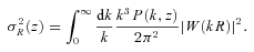
Following this procedure we obtain the PDF of the mass density contrast in redshift space. To obtain that of galaxies we have to further apply a biasing factor. For our purposes here, we simply assume linear deterministic biasing, setting δ_g=bδ (however, see Marinoni et al. 2005). We choose a value ⁠, as required to match the large-scale amplitude of the two-point correlation function of galaxies in our sample, as we shall show in Section 3.

By definition, the PDF described by equation (1) refers to the distribution of δ as measured in randomly placed spheres within the survey volume. On the other hand, for the data we have at our disposal only the conditional values of δ_g as measured in volumes centred on each galaxy in the sample. Given the probabilistic meaning of the distribution function of the density in the two cases they must be related as

4

Being ⁠, the corresponding relation between the PDFs of the density contrast P(δ) is

5

where ⁠.

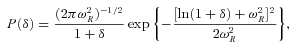
We are then in the position to compare the theoretically predicted P_c (normalized to the total number of galaxies in the sample) to the observed distribution. This is presented in Fig. 1, together with the mean and scatter (68 per cent confidence corridor) of the 24 mock samples. The analytical prediction and the mean of the mocks are in fair agreement (although they disagree in the details at the 1σ level). Note, however, that the detailed shape and amplitude of the analytical prediction are quite sensitive to the choice of the effective redshift of the survey. Here we have used the mean value yielded by the actual redshift distribution d N/d z of the survey, but using e.g. would give a better agreement with the PDF from the simulations. Additionally, the analytical prediction cannot include the small-scale ‘finger-of-God’ effect due to high velocities in clusters (which however has the effect to reduce power on small scales). Finally, it has been computed using the more up-to-date σ₈= 0.8, to check the impact of the value σ₈= 0.9 used for the Millennium Run. Beyond these points, the simple goal of the analytical model is to show an alternative – yet more idealized – example, in addition to the mocks, of what one should expect from the theory. What is relevant for this paper is that the conditional PDF of the data differs strongly from both theoretical predictions. Peaking at δ_g≃− 0.2, it shows an extended high-density tail out to δ_g≃ 7. The distribution expected from the models is more peaked around δ_g= 0 and drops more rapidly for δ_g > 2. This plot clearly shows a statistically significant excess of high-density regions in the galaxy data.4

Figure 1

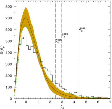
The PDF of the density contrast, measured around each galaxy in the current zCOSMOS 10k catalogue as discussed in the text (histogram). The solid line and shaded area correspond, respectively, to the mean and 1σ dispersion of the same statistics, measured on the 24 Millennium mocks; the dashed curve gives instead, as reference, the expected theoretical distribution for a lognormal model in a ΛCDM cosmology with (Ω_m, Ω_Λ, σ₈) = (0.25, 0.75, 0.8), at the mean redshift of the 10k sample, computed as discussed in the text. The vertical solid lines correspond to values of the density contrast excluding the top 5, 10 and 15 per cent of the distribution.

Open in new tabDownload slide

2.5 Clustering estimation

We estimate real-space galaxy clustering using the standard projected two-point correlation function, w_p(r_p), that properly corrects for redshift-space distortions due to galaxy peculiar motions. This is obtained by projecting the 2D two-point correlation function ξ(r_p, π) along the line of sight5

6

where r_p and π are the components of the galaxy–galaxy separation vector, respectively, perpendicular and parallel to the line of sight (Peebles 1980; Fisher et al. 1994). ξ(r_p, π) is measured using the Landy & Szalay (1993) estimator and properly accounting for the survey selection function and various incompleteness effects, as thoroughly described in de la Torre et al. (2009). Error bars are estimated through the blockwise bootstrap method (e.g. Porciani & Giavalisco 2002; Norberg et al. 2009). This is discussed in detail and compared to results from mock samples in Meneux et al. (2009) and Porciani et al. (in preparation). All clustering codes and methods used here have been extensively tested against independent programs in the course of the latter analyses.

3 RESULTS AND DISCUSSION

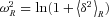
In Fig. 2 we show the projected correlation function w_p(r_p) computed for the 10k sample in the redshift range 0.6 < z < 1 (top curve), together with those from a series of subsamples in which we gradually eliminated galaxies located in the most dense environments. We excluded, respectively, the top 5, 10, and 15 per cent fractions of the distribution of overdensities, corresponding to the dashed vertical lines in Fig. 1. w_p(r_p) for the full 10k sample shows a very flat shape, with significant ‘excess clustering’ above 1 h⁻¹ Mpc, as seen in previous analyses of the COSMOS/zCOSMOS data. When galaxies in the densest environments are excluded, however, the large-scale ‘shoulder’ gradually disappears. What we see is a clear dependence of the mean large-scale clustering of galaxies on the type of environments they inhabit, similarly to the results of Abbas & Sheth (2007) from the SDSS.

Figure 2

The projected two-point correlation function w_p(r_p) of the zCOSMOS 10k at 0.6 < z < 1, compared to subsamples in which galaxies living in the densest environments are gradually excluded (top to bottom). To reduce confusion, error bars are shown for the main sample only, being in general of amplitude comparable to the scatter of the mock samples indicated by the shaded area. The thick solid line and surrounding shaded corridor correspond in fact to the mean and 1σ scatter of the 24 mock surveys. For comparison, the dashed curve also shows the halofit (Smith et al. 2003) analytic prescription for the non-linear mass power spectrum [assuming ΛCDM with (Ω_m, Ω_Λ, σ₈) = (0.25, 0.75, 0.8)], multiplied by an arbitrary linear bias b²= 2.05. The shape of w_p(r_p) for zCOSMOS galaxies agrees with the models when the 10 per cent densest environments are eliminated.

Open in new tabDownload slide

In the same figure we also show the ‘universal’w_p(r_p) expected in the standard ΛCDM cosmological model with linear biasing. The theory predictions are, again, obtained in two ways. First, we use halofit (Smith et al. 2003) to compute directly the approximated non-linear mass power spectrum expected at the survey mean redshift. Secondly, we compute the average and scatter of w_p(r_p) from the 24 mock samples. Remarkably, the two curves (solid and dashed black lines) are virtually indistinguishable above 1 h⁻¹ Mpc once the halofit mass correlation function is properly multiplied by an arbitrary linear bias factor of b²= 2.05. The comparison to the data shows a very good agreement for the 10k subsample in which the 10 per cent densest environments were excluded. We note that the shape of w_p(r_p) measured from the independent VVDS survey shows a shape which is closer to the model predictions (Meneux et al. 2009). With this thresholding in density of the 10k data, therefore, we are able to bring the measured shape of galaxy clustering at z≃ 0.7 from zCOSMOS, VVDS and the standard cosmological model within close agreement, suggesting a more quantitative interpretation of the flat shape of w_p(r_p) observed in zCOSMOS at these redshifts. In previous papers (e.g. Kovač et al. 2009; Meneux et al. 2009) we already suggested that this could be due to the presence of particularly significant large-scale structures between z= 0.5 and 1. Here we see that it is in fact driven by an excess of galaxies sampling high-density regions, skewing the density distribution away from the supposedly ‘universal’ shape. Fig. 3 shows where these high-density galaxies are actually located within the 10k sample. The galaxies belonging to the 10 per cent high-density tail are marked by (red) circles and turn out to belong to a few very well-defined structures only.6 It is easy to imagine that if embedded in a larger volume, these structures would not weight so much as to modify significantly the overall shape of the PDF. As seen from the histogram in Fig. 1, in this volume they produce a clear overabundance of high-density galaxy environments, while regions with average density are under-represented.

Figure 3

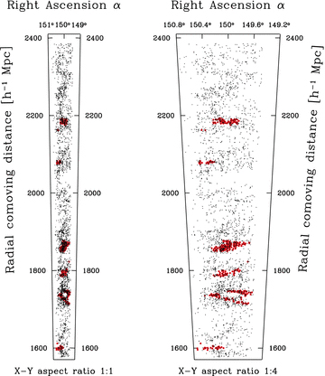
The spatial distribution of galaxies with 0.6 < z < 1 (dots) in the zCOSMOS 10k sample, highlighting those inhabiting the 10 per cent highest density tail of the distribution (circles). These galaxies clearly belong to a few well-defined structures. The right-hand plot is simply an expanded version of the pencil beam on the left-hand side to enhance visibility.

Open in new tabDownload slide

One may wonder, however, whether the theoretical model represented by the Millennium mocks can be taken as a reliable reference. In fact, it has been shown that this specific model tends to overestimate the overall amplitude of w_p(r_p) at z≃ 1 and does not reproduce the observed clustering segregation in colour (e.g. Coil et al. 2008; de la Torre et al., in preparation) In general, semi-analytical recipes do tend to affect the amplitude and shape of the correlation function. This however happens only on small scales, where the complex interplay between galaxy formation processes and the distribution of dark matter haloes has an impact. On large scales instead, they predict a fairly linear biasing, as we can see directly comparing the solid and dashed black lines in Fig. 2. This means that the large-scale shape of the correlation function is essentially driven by the underlying mass distribution in the assumed cosmological model and not by the details of the semi-analytic recipe adopted to generate galaxies. A different recipe would not affect, therefore, the results obtained here, unless we postulate the existence of dramatically non-local galaxy formation processes (e.g. Narayanan, Berlind & Weinberg 2000).

We also note from Fig. 2 that the dependence of w_p(r_p) on the PDF threshold is essentially on large scales. Below ∼ 1 h⁻¹ Mpc there is no significant change when denser and denser environments are excluded. In their analysis of the SDSS, Abbas & Sheth (2007) consider subsamples defined as extrema of the density distribution, i.e. using galaxies lying on the tails of the distribution on both sides. With this selection, they do find a change in w_p(r_p) for different environments also on small scales. It can be shown simply using the conservation of galaxy pairs (see equation 1 of Abbas & Sheth 2007) that the two results are in fact consistent with each other (Ravi Sheth, private communication).

These results highlight the importance in redshift surveys of an accurate reconstruction of the density field to evidence possible peculiarities in the overall PDF as sampled by that specific catalogue. Further strengthening the results obtained by Abbas & Sheth (2007) at z≃ 0, we have shown that an anomalous density distribution function can significantly bias the recovered two-point correlation function, making it difficult to draw general conclusions from its shape. This result provides another example of the intrinsic difficulty existing when comparing observations of the galaxy distribution to theoretical predictions. The theory provides us with fairly accurate forecasts for the distribution of the dark matter and for that of the haloes within which we believe galaxies form (e.g. Mo, Jing & White 1996; Sheth & Tormen 1999). However, translating galaxy clustering measurements into constraints for the halo clustering involves understanding of how the selected galaxies populate haloes with different mass. The result presented here shows how a sample particularly rich in dense structures favours higher mass haloes, which in turn are more clustered, thus biasing the observed correlation function as a function of scale. A more detailed analysis of the environmental dependence of galaxy clustering in the zCOSMOS-bright sample and related HOD modelling will be presented in a future paper.

We thank Ravi Sheth for helpful comments on the manuscript, and M. Kitzbichler and S. White for providing us with the COSMOS mock surveys. LG thanks D. Sanders and the University of Hawaii for hospitality at the Institute for Astronomy, where this work was initiated. Financial support from INAF and ASI through grants PRIN-INAF–2007 and ASI/COFIS/WP3110 I/026/07/0 is gratefully acknowledged.

This work is based on observations undertaken at the ESO–VLT under Large Programme 175.A-0839. Also based on observations with the NASA/ESA Hubble Space Telescope, obtained at the Space Telescope Science Institute, operated by the Association of Universities for Research in Astronomy, Inc. (AURA), under NASA contract NAS 5Y26555, with the Subaru Telescope, operated by the National Astronomical Observatory of Japan, with the telescopes of the National Optical Astronomy Observatory, operated by the Association of Universities for Research in Astronomy, Inc. (AURA), under cooperative agreement with the National Science Foundation and the Canada–France–Hawaii Telescope, operated by the National Research Council of Canada, the Centre National de la Recherche Scientifique de France and the University of Hawaii.

REFERENCES