The slope of the mass profile and the tilt of the Fundamental Plane in early-type galaxies Free

Abstract

1 INTRODUCTION

The global optical properties of giant elliptical galaxies are often parametrized by three key quantities, the effective (half-light) radius (R_e) of the stellar light, the mean surface brightness (or luminosity) and the central line-of-sight velocity dispersion (σ₀). In this three-dimensional parameter space, they occupy a narrow ‘Fundamental Plane’ (Djorgovski & Davis 1987; Dressler et al. 1987), the orientation of which differs significantly from naive expectations from the virial theorem (assuming homology and a constant mass-to-light (M/L) ratio, γ). The relative importance which deviations from homology, variations in the stellar population properties and changing dark matter fractions play in producing this ‘tilt’ have been hotly debated (e.g. Renzini & Ciotti 1993; Hjorth & Madsen 1995; Ciotti, Lanzoni & Renzini 1996; Graham & Colless 1997; Prugniel & Simien 1997; Gerhard et al. 2001; Padmanabhan et al. 2004; Trujillo, Burkert & Bell 2004; Cappellari et al. 2006; Bolton et al. 2007; Tortora et al. 2009, and references therein), with recent work tending to emphasize the importance of dark matter (e.g. Cappellari et al. 2006; Bolton et al. 2007). To maintain the thinness of the Fundamental Plane, however, the dark matter fraction within ∼R_e must be tightly correlated with the optical properties of the galaxy (e.g. Ciotti et al. 1996).

Strong observational evidence for the existence of massive dark matter haloes around early-type galaxies has been provided by independent observational constraints from X-ray studies, lensing and stellar dynamics (e.g. Kochanek 1995; Griffiths et al. 1996; Gerhard et al. 2001; Mathews & Brighenti 2003 and references therein; Humphrey et al. 2006, hereafter H06; Gavazzi et al. 2007; Thomas et al. 2007). Although the total mass distribution within R_e is dominated by the stars, the dark matter fraction is non-negligible, and stellar dynamics and lensing studies (most of which are restricted to within ∼R_e) suggest that it establishes a conspiracy with the luminous matter to produce total mass density (ρ_m) profiles close to ρ_m∝R⁻² (where R is the radius), i.e. the ‘singular isothermal sphere’ (e.g. Kochanek 1995; Kronawitter et al. 2000; Treu & Koopmans 2004; Koopmans et al. 2006, 2009). This ‘bulge–halo conspiracy’ is similar to that which establishes flat rotation curves in disc galaxies.

Total mass distributions approximately consistent with ρ_m∝R⁻² have long been reported from hydrostatic X-ray analysis of nearby elliptical galaxies at scales much larger than R_e (e.g. Thomas 1986; Trinchieri, Fabbiano & Canizares 1986; Serlemitsos et al. 1993; Kim & Fabbiano 1995; Nulsen & Bohringer 1995; Rangarajan et al. 1995; Matsushita et al. 1998) and, in their ROSAT imaging analysis of two galaxies, Buote & Canizares (1994, 1998) actually found an isothermal sphere potential to be preferred over some other mass distributions. With the improved capabilities of Chandra and XMM, much tighter constraints on radial mass profiles have now been reported for a wider array of galaxies (e.g. Buote 2002; O'Sullivan & Ponman 2004; Fukazawa et al. 2006; H06; O'Sullivan, Sanderson & Ponman 2007; Humphrey et al. 2008; Humphrey 2009, hereafter H09), which similarly resemble ρ_m∝R⁻² (as pointed out by Gavazzi et al. 2007), although not exactly so over all radial scales (Romanowsky et al. 2009). Fukazawa et al. (2006) fitted a model of the form ρ_m∝R^−α to the combined mass profiles of their galaxy sample outside 10 kpc, finding α= 1.67 ± 0.33.

At the scale of massive galaxy clusters, hydrostatic X-ray analysis has revealed much less cuspy mass distributions (α∼ 1–1.4; e.g. David et al. 2001; Arabadjis, Bautz & Garmire 2002; Buote & Lewis 2004; Voigt & Fabian 2006). In particular, Lewis, Buote & Stocke (2003) and Zappacosta et al. (2006) studied the very relaxed clusters A 2029 and A 2589, finding that the total mass profiles were in good agreement with the Navarro–Frenk–White (NFW) shape expected for the dark matter only, once again suggesting some kind of conspiracy between the luminous and dark matter to produce an approximately power-law total mass distribution in the core of the system. Stellar dynamics and lensing studies of clusters have, similarly, found less cuspy total mass profiles than would be expected for an unmodified NFW component plus the stellar mass (e.g. Kelson et al. 2002; Sand et al. 2004).

In order to investigate this disparate behaviour at different mass scales, in this paper we carry out a uniform X-ray analysis of a sample of relaxed galaxies, groups and clusters to investigate the shape of the innermost mass distributions. X-ray analysis is ideally suited for this study, since it allows straightforward mass measurements in individual systems over a wide radial range, from the baryon dominated regime (R≲R_e) to regions where the dark matter dominates the gravitating mass (R≫R_e), thus providing adequate leverage to elucidate any conspiracy between these different components. For relaxed systems, hydrostatic equilibrium is believed to be an excellent approximation, with non-thermal effects contributing no more than ∼20 per cent of the total pressure (e.g. Nagai, Vikhlinin & Kravtsov 2007; Churazov et al. 2008; Piffaretti & Valdarnini 2008; H09). In our previous papers (H06; Zappacosta et al. 2006; Gastaldello et al. 2007; H09), we have carried out detailed decompositions of the mass distribution of these systems into baryonic and non-baryonic components. We have not, however, investigated in detail the relationship between these two components. In light of the apparent conspiracies between them at both cluster and galaxy scales, in this present paper, we adopt the more pragmatic approach of examining whether the inner part of the mass profile can be modelled as a power law, and investigating whether its slope varies systematically.

Throughout this work, we assume a cosmology of H₀= 70 km s⁻¹ Mpc⁻¹, Ω_m= 0.3 and Λ= 0.7. All error bars, unless stated otherwise, correspond to 1σ confidence regions.

2 DATA ANALYSIS

2.1 The sample

We chose a sample of nine objects, spanning ∼2 orders of magnitude in virial mass (M_vir) from the survey of morphologically relaxed, X-ray luminous systems by Buote et al. (2007). We supplemented this sample with NGC 1332, which has the smallest R_e of the relaxed systems we have previously studied for X-ray mass analysis (H06; H09). We focused on Chandra data, since high spatial resolution is essential to study in detail the inner part of the X-ray halo. As we require coverage from ≲R_e to several times R_e, we only considered objects which had deep enough data to enable spectra to be obtained in at least two annuli within R_e. Unfortunately, most nearby galaxy clusters which are morphologically relaxed on large scales also exhibit significant active galactic nucleus-induced cavities in the core which complicate the analysis. Therefore, we only included two clusters which have been shown to be relaxed at both large and small scales (Lewis, Stocke & Buote 2002; Zappacosta et al. 2006). The properties of the sample and the archival data we used are summarized in Table 1.

2.2 The slope of the mass profile

The Chandra data were reduced and analysed to provide deprojected temperature and density profiles, as outlined in H09. For NGC 1332, NGC 4261 and NGC 4649, the data are described in H09 and Humphrey et al. (2008). We will discuss in more detail the NGC 720 data in Humphrey et al. (in preparation) and the A 2029 data in Liu, Buote & Humphrey (in preparation). For RXJ1159+5531, we used the deprojected profiles described in Gastaldello et al. (2007; provided by F. Gastaldello, private communication).

Under the hydrostatic approximation, we transformed these density and temperature data into mass constraints by two complementary approaches. First, the ‘traditional’ method involves parametrizing these profiles with arbitrary models (for more details on these models, see Gastaldello et al. 2007; Humphrey et al. 2008; H09) which are then differentiated and inserted into the equation of hydrostatic equilibrium (e.g. Mathews 1978). An advantage of this method is that it makes no a priori assumption about the form of the mass distribution. By evaluating the resulting mass model at a number of radii (corresponding to each spectral extraction region), we obtained the mass ‘data points’ shown for each system in Fig. 1. Error bars were estimated via a Monte Carlo technique (Lewis et al. 2003). We here focus only on the central part of these data; based on experimentation, we considered the mass within 10R_e or 200 kpc, whichever is smaller. Over this radial range, the profiles are all approximately power law in form, but the exact slope varies from object to object.

Figure 1

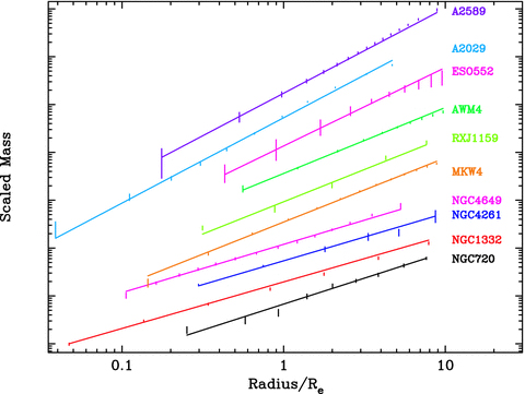
Radial mass profiles for each object, arbitrarily scaled for clarity. The solid lines are the best-fitting profiles determined from our ‘forward fitting’ analysis of the temperature and density profiles, while the data points are determined from the more ‘traditional’ method (Section 2.2). We stress that the models are not fitted to these data points but are derived independently.

Open in new tabDownload slide

We find overall good agreement with previously published mass profiles (Lewis et al. 2003; H06; Zappacosta et al. 2006; Gastaldello et al. 2007; H09), although for ESO552-020 the normalization is ∼0.1 dex higher than that found by Gastaldello et al. (2007), using XMM data. Nevertheless, this discrepancy is comparable with our estimated systematic error for this object (Section 2.3), and will not affect our conclusions.

Since the traditional method relies on the adoption of temperature and density profiles, this can lead to significant systematic errors in the recovered mass distribution (e.g. H09). Furthermore, the individual ‘data points’ are all correlated, which makes it difficult to interpret a fit made directly through them. Therefore, to be more quantitative, we fitted the mass distribution using the ‘forward fitting’ method described in Humphrey et al. (2008). This involves solving the equation of hydrostatic equilibrium to compute temperature and density profile models, given parametrized mass and entropy profiles. Since the entropy profile must rise monotonically, we parametrized it as a constant plus a power law with one or two breaks added, as needed. For the stellar plus dark mass distribution, we adopted a power law, corresponding to ρ_m∝R^−α, i.e.

1

where M is the mass enclosed within radius R. M₇₅ and α are parameters of the fit. An additional gas mass component was included self-consistently in the calculation, but is generally small in the fitted radial range. We fitted only the inner parts of the density and temperature profiles, as described above, freely varying log M₇₅, α, the parameters describing the entropy profile and a term related to the gas pressure at a suitable reference radius (H09). Following H09, parameter space was explored with a Bayesian Monte Carlo method,1 assuming flat priors (see Section 2.3 for the impact of using other priors), and the marginalized best-fitting mass profile parameters and 1σ confidence regions are given in Table 2. Also shown is the χ² per degree of freedom (d.o.f.) for the fits to the temperature and density profiles. In general, the fits are good. For the three objects for which the fits are not formally acceptable (null hypothesis probability <5 per cent), the mean absolute fractional discrepancy between the temperature and density models and the data are less than ∼10 per cent, indicating that the true mass distribution is, nevertheless, very close to a power law in form. For one of these objects (NGC 4261), we did find larger discrepancies within ∼0.5 kpc, but we ignored the data within this region during our fit so as not to bias our results. (It is interesting to note that the full temperature and density profiles of this object can be fitted well by a mass decomposition into luminous and dark matter components: H09.) For the two clusters, we have previously published power-law fits to the central mass distributions, based on other data (Lewis et al. 2003; Buote & Lewis 2004; Zappacosta et al. 2006), and these studies agree well with our results.

In Fig. 1, we overlay the best-fitting models on to the data points obtained from the traditional method, finding overall good agreement. The mean absolute fractional difference between the model and ‘data’ varies from ∼5 to ∼18 per cent, and is smaller than 11 per cent for six objects. While we do not accept a pure power law to be an exact description of the mass profile, these residuals indicate that it is, nevertheless, an excellent approximation to better than ∼10–20 per cent. In fact, the discrepancies we found between the mass profiles determined from both approaches are comparable to the typical systematic uncertainties associated with the traditional analysis method (e.g. H09), so that the actual agreement between the mass distribution and a power-law shape may be even better. From Table 2, it is immediately clear that α systematically varies with mass scale. This is shown explicitly in Fig. 2, where we plot αversus R_e and versusM₇₅, in both cases revealing striking anti-correlations.

Figure 2

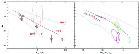
Left-hand panel: variation of the marginalized α as a function of R_e from our data (circles), showing a strong anti-correlation. We overlay (stars) the lensing data of Koopmans et al. (2006), which is computed at scales smaller than ∼R_e and plotted versus R_e. For a strictly fair comparison with our work, their data may need to be shifted slightly to the left (given differences in the adopted photometric bands). We also overlay the predictions of our toy model (solid line; Section 3.2) and an estimate of the model uncertainty (dotted lines). To indicate how changing the Sersic index (n) of the stellar light component affects our model, we have annotated each model line with the corresponding value of n. Right-hand panel: marginalized 1σ joint confidence contours for α and M₇₅ for each object. We overlay the predictions of our toy model, combined with the K-band Kormendy relation (solid line), and an estimate of the uncertainty in the model (dotted lines).

Open in new tabDownload slide

2.3 Systematic errors

As in all studies of dark matter in early-type galaxies, regardless of the specific method, our work involved a number of arbitrary analysis choices. In this section, we describe how sensitive our results are to the various choices we made. For a more detailed discussion of these various systematic error assessments, see H09.

We first examined how the choice of priors might be influencing our results by replacing each of the flat priors we adopted by priors which were flat in logarithmic space (we replaced the flat prior on log M₇₅ with one which is flat on M₇₅). These choices typically had a smaller effect than the statistical errors. Next we investigated the sensitivity of our spectral-fitting results to our treatment of the Chandra background by using the standard ‘background template’ spectra, suitably renormalized to match the data at energies ≳10 keV, instead of the more robust, modelled background adopted by default. To assess the importance of the radial range we fitted, we tried reducing it by ∼20 per cent for each object. We experimented with spectral-fitting over different energy ranges (0.4–7.0, 0.5–2.0 and 0.7–7.0 keV, in addition to our default, 0.5–7.0 keV), varying the neutral galactic column density by 25 per cent, and the distance by 30 per cent (for the New General Catalogue objects, we instead varied the distance by the statistical error on their distance measurements in Tonry et al. 2001). In Table 2, we list the largest change in the marginalized parameter values arising due to these choices. None of these systematic errors is large enough to affect our conclusions.

3 DISCUSSION

3.1 A luminous–dark matter conspiracy

In general, the stars are believed to dominate the gravitational potential within ∼R_e, with the dark matter dominating outside this scale (e.g. Brighenti & Mathews 1997; Gerhard et al. 2001); in particular, we have shown this for the systems studied here (Lewis et al. 2003; Buote & Lewis 2004; H06; Zappacosta et al. 2006; Gastaldello et al. 2007; H09). Therefore, the approximately power-law mass distributions shown in Fig. 1 indicate an apparent conspiracy between the luminous and dark matter to produce a scale-free total mass distribution, at least within ∼10R_e. At much larger scales, there is evidence that the profiles deviate from this simple shape (e.g. Lewis et al. 2003; H06; Vikhlinin et al. 2006; Gastaldello et al. 2007; Romanowsky et al. 2009). Nevertheless, in the inner regions of the systems, this effect is similar to the ‘bulge–halo’ conspiracy found at much smaller scales (≲R_e) in lensing and stellar dynamics studies (e.g. Treu & Koopmans 2004; Koopmans et al. 2006, 2009). It is important to appreciate that the observed power-law mass profiles cannot simply arise from the arbitrary superposition of any reasonable stellar and dark mass components. To illustrate this quantitatively, we simulated a power-law-like mass profile and fitted it with a model comprising Sersic and dark matter components (as described in detail in Section 3.2). For any given galaxy luminosity, we found that both R_e and the normalization of the dark matter component cannot vary by more than ∼25 per cent from their ‘best’ values while maintaining mean absolute fractional deviations between the model and data of less than 10 per cent (as indicated by our fits in Section 2.2).

The origin of this conspiracy is unclear, but it is likely tied to the complex interaction of baryons and dark matter in the centres of galaxies (for example, Robertson et al. 2006 point out the importance of gas physics in maintaining the tilt of the Fundamental Plane, which may be related to this conspiracy; Section 3.3). Unfortunately, these processes are very poorly understood; the predicted central dark matter density cusps due to ‘adiabatic contraction’ (Blumenthal et al. 1986; Gnedin et al. 2004) have not been observationally confirmed (e.g. H06; Zappacosta et al. 2006; Dutton et al. 2007; Gnedin et al. 2007), suggesting that other effects, such as dynamical friction, may be important (e.g. El-Zant et al. 2004; Dutton et al. 2007; Abadi et al. 2009). It is unclear, therefore, that any model is so far robustly predicting a power-law total mass distribution arising from these effects.

Since the data were not all fitted over the same physical scales, it is important to assess whether the systematic variation in α we observe is simply an artefact of these different fit ranges. In Fig. 3, we show the mass profiles of three representative systems with different R_e, arbitrarily scaled for clarity, and shown as a function of physical radius (left) and fraction of the virial radius (right; deduced from the virial masses reported in Buote et al. 2007). In conjunction with Fig. 1 (which shows the same profiles as a function of fraction of R_e), it is immediately clear that throughout overlapping radial scales the slopes of the three mass distributions are all very different, so that the fit range is unlikely to be the cause of the trends observed in Fig. 2.

Figure 3

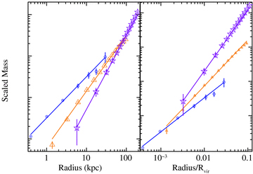
Left-hand panel: comparison of the mass profiles of NGC 4261 (circles), MKW4 (triangles) and A 2589 (stars), normalized to have the same mass at 100 kpc. Note that the shapes of the mass profiles are different even over overlapping radial ranges. Right-hand panel: the same, but scaling the radius with respect to the virial radius (R_vir) and renormalizing each profile to have the same mass at 0.001R_vir.

Open in new tabDownload slide

Although all of the systems we considered are morphologically relaxed, which should eliminate objects with the largest departures from hydrostatic equilibrium, it is still important to consider whether deviations from hydrostatic equilibrium could be responsible for the observed trends. In order to affect the shape of the mass profile, any source of non-thermal pressure must vary radially in a finely balanced manner, given that the gas pressure profile is consistent with a power-law mass density profile (Fig. 1) that varies systematically with the host properties (Fig. 2). For the cluster A 2589, Zappacosta et al. (2006) concluded that, if the true mass distribution is much cuspier than inferred from the X-rays (for example, an unmodified NFW plus a stellar mass component), no plausible source of turbulent or magnetic pressure could make the X-ray measurements imply such a flat total density profile. H09 carried out full mass decompositions for three of our galaxies, finding stellar M/L ratios in excellent agreement with the predictions of stellar population synthesis models, suggesting that non-thermal pressure is very small (≲10–20 per cent) within R_e. This was further supported by the good agreement between the X-ray constraints on the central black hole masses and those obtained from optical methods for these objects. Furthermore, nine of our objects were included in the sample of Buote et al. (2007), who showed that their dark matter haloes inferred from X-ray mass analysis approximately exhibit the relationship between halo ‘concentration’ (c_vir) and total mass predicted from numerical structure formation simulations. This supports the idea that the shapes of the mass profiles for these systems are not significantly in error due to non-hydrostatic effects.

In their survey of 15 lensing systems, Koopmans et al. (2006) found that α ranged from ∼1.8 to 2.4, while the R_e spanned ∼2–17 kpc. In the left-hand panel of Fig. 2, we overlay their measured αversus R_e. We find that they are roughly consistent with the points from our X-ray sample, but at given R_e, α is generally larger. For strict consistency with our adopted photometric bands, their data may need to be adjusted, however. Since R_e in the K band is typically smaller than in bluer bands (as an illustration of this effect, for the galaxies in the catalogue of La Barbera et al. 2008, we find that R_e is on average ∼50 per cent larger in the R band than in the K band), this would likely involve shifting the Koopmans et al. to the left, bringing them into better agreement with our results. By inspection, there is a slight hint in their data of the anti-correlation we observe between α and R_e, although it is not statistically significant. However, since their fits were all restricted to regions ≲0.9R_e, where the stellar mass dominates the potential, they are more likely to have been subject to local curvature in the mass distribution than the X-ray data were, given the better radial coverage of the latter.

3.2 Decomposing the mass profiles: a toy model

To investigate quantitatively the implications of the apparent conspiracy between dark and luminous mass components implied by Fig. 1, we constructed a simple toy model by decomposing a pure power-law mass distribution into an NFW (Navarro, Frenk & White 1997) dark matter profile plus a de Vaucouleurs stellar mass component (using the deprojected Sersic approximation of Prugniel & Simien 1997, and fixing the Sersic index, n= 4). In our previous work (H06; Zappacosta et al. 2006; Buote et al. 2007; Gastaldello et al. 2007; H09), we have shown that decompositions of this type for the systems studied in the present work give parameters for the NFW model which are consistent with theory. The measured NFW concentration parameters are slightly higher than predicted median from N-body simulations, but this can be reasonably attributed to relaxed X-ray selected systems having formed early. To perform the decomposition, we first constructed a set of mass ‘data points’ from the power-law model in 10 approximately logarithmically spaced bins between ∼0.4 and 200 kpc, which we then fitted with the two-component model by minimizing the rms of the fractional residuals. The normalization and scale radius of the dark matter component were allowed to vary freely, as were R_e and the normalization of the stellar model. We allowed the slope of the input mass distribution to vary systematically from α= 2.2 to 1.35. Below this limit, we found that the derived relationships (discussed below) became non-monotonic, which may represent the limitations of our simple parametrization rather than any physical insight, and so we prefer not to discuss this regime. While one might a priori expect significant degeneracies in this decomposition given the number of free parameters, in fact the shapes of the Sersic and NFW mass profiles are sufficiently different that we found a unique decomposition for any input power law, at least for the range of profiles and models we investigated. We show an example simulated profile, and the best-fitting dark and stellar mass components, in Fig. 4, clearly illustrating how they can conspire to produce an approximately scale-free model.

Figure 4

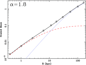
Sample simulated mass profile and associated mass decomposition. The data points correspond to a power-law mass distribution with α= 1.8, while the solid line indicates the best-fitting two-component (dark plus luminous matter) model. Error bars, corresponding to a 10 per cent fractional uncertainty, are shown to guide the eye. Also shown are the corresponding best-fitting dark matter (dotted line) and stellar mass (dashed line) models. Note how the sum of two scale-dependent models produces an approximately power-law total mass distribution over the fitted range.

Open in new tabDownload slide

We overlay in Fig. 2 (left-hand panel) the best-fitting relation between R_e and α obtained from our simple mass decompositions (solid line), which can be approximated to better than 1 per cent by α= 2.31 − 0.54 log R_e. Without any fine tuning, it clearly captures the overall behaviour of the observed data reasonably well. Since the stellar light profiles of real galaxies may not be exactly de Vaucouleurs in form, we have also experimented with varying the Sersic index, n, from 3 to 5. Similarly, the NFW model used to parametrize the dark matter halo over the fitting range may not be strictly correct if the baryonic and non-baryonic components interact gravitationally. Therefore, we have tried replacing it with the revised mass model of Navarro et al. (2004), allowing the mass slope index to fit freely and thus provide more freedom in parametrizing the radial distribution of dark matter. The dotted lines in Fig. 2 bound the range of recovered relations, given these changes, which clearly bracket the observed data. In practice, the impact of changing the stellar light profile dominated this estimate of our model uncertainty.

Since our simple toy model can be freely renormalized, we cannot use it alone to make any explicit predictions for the relationship between α and M₇₅. One way to make further progress, however, is to exploit the ‘Kormendy relation’ between a galaxy's luminosity and R_e (Kormendy 1977). For a given stellar M/L ratio (γ_*), M₇₅ must be adjusted to keep the stellar component consistent with the Kormendy relation while maintaining the power-law total mass distribution for a given α (and hence R_e). We adopted a form for this relation which is appropriate for our data, estimated from the K-band galaxy luminosities and R_e tabulated by Gastaldello et al. (2007) and H06. We found a mean relation log L/L_⊙= 10.95 + 0.79 log R_e, with an intrinsic scatter of ∼0.11 dex, where L is the total luminosity of the galaxy in the K band and L_⊙ is the luminosity of the Sun, assuming a K-band absolute solar magnitude of 3.41. We assumed γ_*= 1, appropriate for an old stellar population (e.g. Maraston 2005). In Fig. 2 (right-hand panel), we overlay the predictions of this simple model (solid line), and an estimate of the range of uncertainty, which factors in the effects of varying the Sersic index of the stellar light by ±1, the intrinsic scatter in the Kormendy relation and a ±50 per cent variation in γ_* (which dominates the error budget). Clearly, the model captures the overall behaviour of the data fairly well.

To verify that our model is self-consistent, it is important to determine if the parameters of the fitted dark matter model it predicts are reasonable. Since the toy model cannot be used alone to set the normalization of the mass profile, to do this we considered the simple model, folding in the Kormendy relation, described above. Starting with the α–M₇₅ relation predicted by this model, we simulated corresponding power-law mass profiles, and decomposed them into Sersic and dark matter components. We found monotonic relations between M_vir and α and between NFW c_vir and α, allowing us to recast this as a c_vir–M_vir relation, which we can approximate by c_vir=c₁₄(M_vir/10¹⁴ M_⊙)^−β, where c₁₄= 10 and β= 0.17. This is very close to the best-fitting c_vir–M_vir relation found by Buote et al. (2007), for which c₁₄= 9.0 ± 0.4 and β= 0.172 ± 0.026. Exploring the estimated range of uncertainty on the model linking α and M₇₅, we found c₁₄ to lie in the range 6–16 and β from 0.13 to 0.18. The total range of M_vir spanned by our predicted c_vir–M_vir relation (∼12.5 < log₁₀M_vir < 15.0) is similar to the range spanned by the systems in our sample. It appears, therefore, that the parameters of the NFW component implied by our simple model are appropriate for the kinds of system studied in this work.

3.3 Implications for the Fundamental Plane

The existence of a conspiracy between the dark and luminous matter to produce a power-law total mass profile should have implications for the tilt of the Fundamental Plane. The Fundamental Plane may be written in the form

2

where σ₀ is the central velocity dispersion, μ is the mean surface brightness within R_e and A and B are proportionality constants. One way to gain insight into this relation is to interpret it in terms of the scalar virial theorem (e.g. Binney & Tremaine 2008). We can write this in the form

Here, R_e is in kpc, σ₀ is in km s⁻¹, L_1/2 is (approximately) the light within R_e (in solar units) and γ=γ_*γ_m is the M/L ratio in solar units, where γ_* is the stellar M/L ratio and γ_m the ratio of total mass to stellar mass within R_e. The value of the additive constant on the right-hand side is useful only in setting the absolute normalization of γ_* and does not affect our conclusions. For convenience, we chose to determine it from the theoretical relation of Wolf et al. (2009),2 since this implies a mean γ_* of ∼1 for the La Barbera et al. (2008) galaxy sample (see below), which is consistent with the expectations for an old stellar population. Alternative, empirical relations have been found by Cappellari et al. (2006, assuming mass follows light) and Bolton et al. (2007, assuming a singular isothermal sphere mass distribution), which would imply lower γ_*, by as much as ∼40 per cent (for the Cappellari et al. relation). Nevertheless, for our work the absolute value of γ_* is unimportant, and so this choice does not affect our conclusions.

In the K band, assuming the absolute solar magnitude is 3.41 and neglecting cosmological effects, we can write log (L_1/2/πR²_e) ≃ 16.00 − 0.4μ, and hence

3

If structural non-homology does not significantly affect this equation, the tilt of the Fundamental Plane arises through the dependence of γ on the other properties of the galaxy. Eliminating σ₀ between equations (2) and (3) and rearranging, we obtain

4

where we have used the ‘log σ₀ fit’ values for A and B from the recent K-band analysis of La Barbera et al. (2008). The μ term is consistent with zero, within the error, suggesting that the tilt of the Fundamental Plane can arise if γ depends only on R_e, which is exactly the prediction of the toy model, as we discuss below. Nevertheless, since the μ term may be non-negligible, to obtain a more accurate assessment of how γ varies with R_e, we computed log γ directly from the data of La Barbera et al. by using equation (3). We grouped these data into a series of narrow R_e bins,3 within each of which we calculated the mean γ and its error (by applying the central limit theorem to the scatter of the data), as shown in Fig. 5.

Figure 5

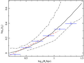
The predicted ratio between the total mass and stellar mass enclosed within R_e from our toy model (γ_m), shown as a function of R_e (solid line). The dot–dash lines indicate our estimate of the uncertainty on the model, and the dashed line indicates the best-fitting linear approximation in the range log R_e= 0.2 –1.0. The data points are the observed K-band M/L ratios from the data of La Barbera et al. (2008) (see text). Note the good agreement between the data and the toy model.

Open in new tabDownload slide

We can use our toy model not only to predict the relationship between R_e and α, but also the dark matter fraction within R_e (and hence γ_m), as is immediately clear from inspection of Fig. 4. Since the dark matter fraction does not depend on the overall normalization of the mass profile, we do not need to fold in any other relations (such as the Kormendy relation). Furthermore, since we find that R_e varies monotonically with α (Fig. 2), it is possible to recast this as a relation between γ_m and R_e. We show the resulting relation [roughly log γ_m≃− 0.03 log R_e+ 0.32 (log R_e)²] in Fig. 5, along with an estimate of the uncertainty that arises from varying the Sersic index by ±1, or adopting the Navarro et al. (2004) model for the dark matter profile. It is immediately clear that there is good agreement between the model and the La Barbera et al. (2008) data, implying the mean γ_*≃ 1, as noted above. Since the stellar populations of early-type galaxies (and hence γ_*) do not strongly vary with R_e (at least for R_e≳ 1 kpc: Graves, Faber & Schiavon 2009), this suggests that assuming the ubiquity of approximately power-law density profiles (supported by Fig. 1) is sufficient (albeit not necessary) to explain the tilt of the Fundamental Plane. While it is possible that not all giant early-type galaxies have density profiles which so closely resemble a power law (although we are not aware of any convincing such counter-examples found by X-ray methods) to lie on the Fundamental Plane, Fig. 5 indicates that their γ_m must still vary with R_e in a very similar way to the predictions of the toy model. Nevertheless, since it is actually the flattening of the density profile with increasing R_e that is responsible for the γ_m–R_e relation predicted by the toy model, it is plausible that similar flattening of the mass distributions in a system without a power-law-like mass distribution might produce approximately the same trend.

One intriguing prediction of our toy model is that the relationship between log γ_m and log R_e has some curvature, which would also imply curvature in the Fundamental Plane. There is, in fact, some evidence that brightest cluster galaxies (BCGs) may not lie on the same Fundamental Plane as smaller systems (e.g. Oegerle & Hoessel 1991; Bernardi et al. 2007; von der Linden et al. 2007), but it is not clear that the observed behaviour could be explained in terms of the predicted curvature. Indeed, there is a hint that the observed γversus R_e relation begins to deviate from our simple predictions at R_e≳ 20 kpc (Fig. 5), which may arise due to deviations from structural homology among BCGs, or it may represent the limitations of our simple model.

To make a more quantitative comparison between the traditional Fundamental Plane and our toy model, we adopted a linear approximation for the toy model relationship between γ_m and R_e (log γ_m≃− 0.11 + 0.37 log R_e; this is accurate to about ∼0.03 dex over the range 0.2 < log R_e < 1.0, as shown in Fig. 5, assuming γ_*= 1). Substituting this into equation (3) (assuming γ_* is constant) and rearranging into the form of equation (2), we found A= 1.46 and B= 0.29. These are in good agreement with recent K-band measurements of the Fundamental Plane (A∼ 1.4–1.5 and B∼ 0.30–0.33; Pahre, Djorgovski & de Carvalho 1995; Mobasher et al. 1999; Jun & Im 2008; La Barbera et al. 2008). Repeating the analysis, but allowing the Sersic index to vary by ±1, or using the alternative dark matter model of Navarro et al. (2004), we obtained A in the range ∼1.2–1.6 and B≃ 0.23–0.31. Thus, assuming only a power-law total mass distribution, we can clearly reproduce the shape of the K-band Fundamental Plane, without any fine tuning of the model parameters. We therefore speculate that the establishment of a power-law total mass distribution is a fundamental feature of galaxy formation and the principal factor in determining the tilt of the Fundamental Plane. Since the relative importance of gas-rich and ‘dry’ merging for the assembly of present-day giant ellipticals is still under debate (e.g. Hopkins, Cox & Hernquist 2008; Naab, Johansson & Ostriker 2009; Nipoti et al. 2009), the requirement of producing a nearly power-law total mass distribution in the core of low-redshift systems will therefore be a key test of these models.

We thank Fabio Gastaldello and Wenhao Liu for making available their deprojected density and temperature profiles. We thank Bill Mathews, Chris Fassnacht and Luca Ciotti for stimulating and helpful discussions. We also thank Fabio Gastaldello and Michele Cappellari for providing comments on a draft of the paper. This research made use of the NASA/IPAC Extragalactic Data base (NED) which is operated by the Jet Propulsion Laboratory, California Institute of Technology, under contract with NASA. Partial support for this work was provided by NASA under grant NNG04GE76G issued through the Office of Space Sciences Long-Term Space Astrophysics Program.

REFERENCES