


Abstract
In addition to the maximum likelihood approach, there are two other methods that are commonly used to reconstruct the true redshift distribution from photometric redshift data sets: one uses a deconvolution method, and the other a convolution. We show how these two techniques are related, and how this relationship can be extended to include the study of galaxy scaling relations in photometric data sets. We then show what additional information photometric redshift algorithms must output so that they too can be used to study galaxy scaling relations, rather than just redshift distributions. We also argue that the convolution-based approach may permit a more efficient selection of the objects for which calibration spectra are required.
1 INTRODUCTION
The next generation of sky surveys will provide reasonably accurate photometric redshift estimates, so there is considerable interest in the development of techniques that can use these noisy distance estimates to provide unbiased estimates of galaxy scaling relations. While there exist a number of methods for estimating photometric redshifts (Budavári 2009 and references therein), there are fewer for using these to estimate accurate redshift distributions (Padmanabhan et al. 2005; Sheth 2007; Lima et al. 2008; Cunha et al. 2009), the luminosity function (Sheth 2007) or the joint luminosity–size, colour–magnitude, etc. relations (Rossi & Sheth 2008; Christlein et al. 2009; Rossi, Sheth & Park 2010).
Ideally, the output from a photometric redshift estimator is a normalized likelihood function that gives the probability that the true redshift is z given the observed colours (i.e. Bolzonella, Miralles & Pelló 2000; Collister & Lahav 2004; Cunha et al. 2009). Let  denote this quantity; it may be skewed, bimodal or more generally it may assume any arbitrary shape.
Let ζ denote the mean or the most probable value of this distribution (it does not matter which, although some of the logic that follows is more transparent if ζ denotes the mean). Often, ζ (sometimes with an estimate of the uncertainty on its value) is the only quantity that is available. Therefore, in Section 2.1 we first consider how ζ compares with the true redshift z, and contrast the convolution and deconvolution methods for estimating dN/dz, while in Section 2.2 we describe how to reconstruct the redshift distribution directly from colours. Section 2.3 shows what this implies if one wishes to use the full distribution  . Section 2.4 shows how to extend the logic to the luminosity function, and Section 2.5 to scaling relations, again by contrasting the convolution and deconvolution methods, and showing what generalization of
  is required from the photometric redshift codes if one wishes to do this. A final section summarizes our results.
Where necessary, we write the Hubble constant as H0= 100 h km s−1 Mpc−1, and we assume a spatially flat cosmological model with (ΩM, ΩΛ, h) = (0.3, 0.7, 0.7), where ΩM and ΩΛ are the present-day densities of matter and cosmological constant scaled to the critical density.
2 TO CONVOLVE OR TO DECONVOLVE?
In what follows, we will use spectroscopic and photometric redshifts from the Sloan Digital Sky Survey (SDSS) to illustrate some of our arguments. Details of how the early-type galaxy sample was selected are in Rossi et al. (2010); the photo-zs for this sample are from Csabai et al. (2003).
2.1 The redshift distribution
Suppose that the true redshifts z are available for a subset of the objects; for now, assume that the subset is a random subsample of the objects in a magnitude-limited catalogue. Ideally, this subset would have the same geometry as the full survey, as cross-correlating objects with spectra and those without allows the use of other methods (e.g. Caler, Sheth & Jain 2009). In practice, this may be difficult to achieve – and this is not required for the analysis that follows, provided that the photometric redshift estimator does not have spatially dependent biases (e.g. as a result of photometric calibrations varying across the survey).
For objects with spectroscopic redshifts, one can study the joint distribution of ζ and z (see Fig. 1). Typically, most photometric redshift codes are constructed to return 〈ζ|z〉≈z. The codes that do so are sometimes said to be unbiased, but they are not perfect: the scatter around the unbiased mean is of order σζ|z≈ 0.05(1 +z). This scatter, combined with the fact that 〈ζ|z〉≈z, means that 〈z|ζ〉≠ζ: the fact that 〈z|ζ〉 is guaranteed to be biased is not widely appreciated. However, we show below that it matters little whether 〈ζ|z〉 or 〈z|ζ〉 is unbiased; what matters is whether the bias is accurately quantified.
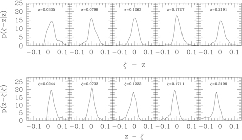
Distribution of the difference between spectroscopic and photometric redshifts (z and ζ), at fixed z (top) and ζ (bottom), in the SDSS early-type galaxy sample. Note that p(ζ|z) is rather well centred on z, whereas p(z|ζ) is not centred on ζ.
 and dN/dz denote the distribution of ζ and z values in the subset of the data where both z and ζ are available, then what matters is that p(ζ|z) and p(z|ζ), where

 is measured in the full data set, and p(ζ|z) is known, a deconvolution is then used to estimate the true dN/dz.
Rossi et al. (2010) have shown that the deconvolution method accurately reconstructs the true dN/dz distribution from  . Fig. 2 shows that the convolution approach also works well, even when only a random 5 per cent of the full data set is used to calibrate p(z|ζ), as displayed in Fig. 1. Thus, for the data set in which both z and ζ are available, both the convolution and deconvolution approaches are valid, whether or not the means (or, for that matter, the most probable values) of p(z|ζ) and p(ζ|z) are unbiased, and however complicated (skewed, multimodal) is the shape of these two distributions. This remains true in the larger data set, where only ζ is known. However, whereas the convolution approach assumes that p(z|ζ) is the same in the calibration subset as in the full one, the deconvolution approach assumes that p(ζ|z) is the same.
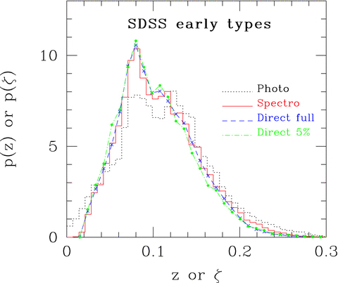
Distribution of  (dotted) and dN/dz (solid); crosses show the result of convolving
  with p(z|ζ) (from the bottom panel of Fig. 1).
2.2 Convolution directly from colours
Although we arrived at equation (5) by requiring the mapping c→ζ to be one-to-one [as may be the case for e.g. luminous red galaxies (LRGs)], it is actually more general. This is because one can simply measure p(z|c) in the sample for which spectra are in hand, for the same reason that one could measure p(z|ζ). In fact, p(z|c) is an easier measurement, since it does not depend on the output of a photo-z code! The constraint on the mapping between c and ζ in the discussion above was simply to motivate the connection between photo-z codes and the convolution method. Once the connection has been made, however, there is no real reason to go through the intermediate step of estimating ζ, since all photo-z codes use the observed colours c anyway. In this respect, equation (5) is the more direct and natural expression to work with than is equation (4). In particular, because p(z|c) is an observable, the convolution approach of equation (5) is independent of any photo-z algorithm. Of course, if this method is to work, then the subsample with spectral information must be able to provide an accurate estimate of p(z|c).
2.3 Relation to photo-z algorithms
The convolution method of the previous subsection provides a simple way of illustrating how one should use the output from photo-z codes that actually provide a properly calibrated probability distribution  for each set of colours c, to estimate dN/dz. It also shows in what sense the codes should be ‘unbiased’.
 . This is because
 does not have the same shape as p(z|c), then use of
  will lead to a bias; this is the pernicious bias that must be reduced – whether or not 〈z|c〉 equals the spectroscopic redshift is, in some sense, irrelevant. (In the case of a one-to-one mapping between c and ζ, 〈z|c〉 is the same as the quantity 〈z|ζ〉, which we have discussed in the previous subsections.)
Satisfying  is non-trivial. This is perhaps most easily seen by supposing that the template or training set consists of two galaxy types (early- and late type, say), for which the same observed colours are associated with two different redshifts. In this case, if the photo-z algorithms are working well, then
  will be bimodal for at least some c. However, if the sample of interest only contains LRGs, then p(z|c) may actually be unimodal. As a result,
  unless proper priors on the templates are used, or care is taken to ensure that the training set is representative of the sample of interest.
2.4 The luminosity function
 to denote the absolute magnitude estimated using the photometric redshift ζ, and M its correct value, then
 and the assumption that
  , measured in a subset for which both z and ζ (hence both M and
  ) are available, also applies to the full photometric survey.
 , and then used the fact that
 ; note that this weight depends on
  . Fig. 3 shows
  and
and  ; notice how broad they are, and how much more skewed and biased
  is than
  . Nevertheless, Rossi et al. (2010) have shown that the deconvolution algorithm produces good results. Fig. 4 shows that the convolution algorithm works equally well.
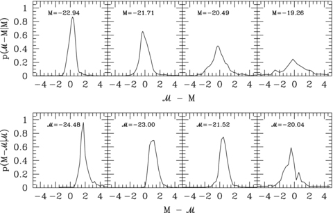
Similar to Fig. 1 but for the true absolute magnitude and the estimate from the photometry. Notice that  is approximately symmetrically distributed around M, whereas
  can be both significantly offset from
  and skewed.

 , so the expression above shows explicitly why should the photometric errors be thought of as affecting N(M) and not φ(M).
 , it is worth considering how one computes M from z given the observed colours c. If there were no k-correction, then the luminosity in a given band would be determined from the observed apparent brightness by the square of the (cosmology dependent) luminosity distance – the colours are not necessary. In practice, however, one must apply a k-correction; this depends on the spectral type of the galaxy, and hence on its colour. As a result, the mapping between m and M depends on z and c. However, it is still true that both M and z are determined by c. Therefore, the spectroscopic subsample that was previously used to estimate p(z|c) also allows one to estimate p(M, z|c). The quantity of interest in the previous section, p(z|c), is simply the integral of p(M, z|c) over all M. The quantity of interest here, p(M|c), is the integral of p(M, z|c) over all z. Thus, equation (8) becomes
 : the quantity such codes currently output,
  , is the integral of
  over all M. The relevant weighted sum becomes
 is the integral of
  over all z, the sum is over all the objects in the catalogue, and the method only works if
  .
.
 ; this is easily computed from distributions like those shown in the bottom panel of Fig. 3. The final expression writes this as a sum over the observed distribution of colours.
2.5 Galaxy scaling relations
 , where M is a set of absolute luminosities (typically, these will be those associated with the various bandpasses from which the colours c were determined). Hence, the colour–magnitude relation, which is really a statement about the joint distribution in two bands, can be estimated by
 .
.3 DISCUSSION
We showed how previous work on deconvolution algorithms for making unbiased reconstructions of galaxy distributions and scaling relations (Sheth 2007; Rossi & Sheth 2008; Rossi et al. 2010) could be related to convolution-based methods. Whereas deconvolution-based methods require accurate knowledge of p(ζ|z), the distribution of the photometric redshift ζ given the true redshift z, convolution-based methods require accurate knowledge of p(z|ζ). Since ζ is derived from photometry, this may more generally be written as p(z|c), where c is the vector of observed photometric parameters that were used to estimate the redshift. In both cases, p(z|c) and p(ζ|z) are calibrated from a sample in which z is known, and are then used in a larger sample where z is not available. If the smaller training set has the same selection limits as the larger data set (e.g. both have the same magnitude limit), then both approaches are valid. We have illustrated our arguments with measurements in the SDSS (Figs 1–4).
We also showed what additional information must be output from photometric redshift codes if their results are to be used in a convolution-like approach to provide unbiased estimates of galaxy scaling relations. In particular, we argued that only if the redshift distribution output by a photo-z algorithm,  , has the same shape as p(z|c), can the algorithm be said to be unbiased. Only in this case its output (available for the full sample) can be used in place of p(z|c) (which is typically available for a small subset). The safest way to accomplish this is for the training set to be a random subsample of the full data set – and to then tune the algorithm so that
  . If the training set is not representative, then care must be taken to ensure that
  does not yield biased results.
Obtaining spectra is expensive, so the question arises as to whether or not there is a more efficient alternative to the random-sample approach. For the convolution method, which requires p(z|c), the answer is clearly ‘yes’. This is because some colour combinations (e.g. the red sequence) might give rise to a narrow p(z|c) distribution, whereas others may result in broader distributions. Since it will take fewer objects to accurately estimate the shape of a narrow p(z|c) distribution than that of a broad one, observational effort would be better placed in obtaining spectra for those objects that produce broad p(z|c) distributions. For the deconvolution approach, one would like to preferentially target those redshifts z that produce broader p(ζ|z) distributions – for similar reasons. However, since z is not known until the spectra are taken, this cannot be done, so taking a random sample of the full data set is the safest way to proceed.
Our methods permit accurate measurement of many scaling relations for which spectra were previously thought to be necessary (e.g. the colour–magnitude relation, the size–surface brightness relation, the photometric Fundamental Plane), so we hope that our work will enable photometric redshift surveys to provide more stringent constraints on galaxy formation models at a fraction of the cost of spectroscopic surveys.
RKS thanks L. Da Costa, M. Maia, P. Pellegrini, M. Makler and the organizers of the DES Workshop in Rio in 2009 May where he had stimulating discussions with C. Cunha and M. Lima about the relative merits of convolution and deconvolution methods, and the APC at Paris 7 Diderot and MPI-Astronomie Heidelberg, for hospitality when this work was written up.
Funding for the SDSS and SDSS-II has been provided by the Alfred P. Sloan Foundation, the Participating Institutions, the National Science Foundation, the US Department of Energy, the National Aeronautics and Space Administration, the Japanese Monbukagakusho, the Max Planck Society and the Higher Education Funding Council for England. The SDSS Web site is http://www.sdss.org/.
The SDSS is managed by the Astrophysical Research Consortium for the Participating Institutions. The Participating Institutions are the American Museum of Natural History, Astrophysical Institute Potsdam, University of Basel, University of Cambridge, Case Western Reserve University, University of Chicago, Drexel University, Fermilab, the Institute for Advanced Study, the Japan Participation Group, Johns Hopkins University, the Joint Institute for Nuclear Astrophysics, the Kavli Institute for Particle Astrophysics and Cosmology, the Korean Scientist Group, the Chinese Academy of Sciences (LAMOST), Los Alamos National Laboratory, the Max-Planck-Institute for Astronomy (MPIA), the Max-Planck-Institute for Astrophysics (MPA), New Mexico State University, Ohio State University, University of Pittsburgh, University of Portsmouth, Princeton University, the United States Naval Observatory and the University of Washington.
REFERENCES
