popstar evolutionary synthesis models II: optical emission-line spectra from giant H ii regions Free

Abstract

1 INTRODUCTION

H ii regions have been widely studied for the last three decades (Pagel, Edmunds & Smith 1980; Evans & Dopita 1985; Dopita & Evans 1986; Díaz et al. 1987; Vílchez et al. 1988; Díaz et al. 1991; Díaz 1994). In those studies, the functional parameters, such as ionization parameter, effective temperature of the ionizing stars and oxygen abundance, were translated into physical parameters associated to the star clusters (mass, age and metallicity). In order to do this, several grids using evolutionary models plus photoionization codes were computed by our group (García Vargas & Díaz 1994; García-Vargas, Bressan & Díaz 1995a,b; García-Vargas, Mollá & Bressan 1998) and others (Stasińska 1978, 1980; Stasińska et al. 1981; Stasińska 1982, 1990).

In the last decade, the evolutionary synthesis technique has been improved with the inclusion of updated stellar tracks or isochrones, the use of better stellar spectra as input for the codes, a better treatment of binary stars, a wider wavelength coverage and a higher spectral resolution. Codes like starburst99 (Leitherer et al. 1999) use the Geneva group stellar tracks and are tuned for star-forming regions. On the contrary, codes like pegase (Fioc & Rocca-Volmerange 1997) or galaxev (Bruzual & Charlot 2003) are specially computed for intermediate and evolved populations and use the Padova group stellar tracks. These codes, among others, have been intensively applied to spectrophotometric catalogues to derive the physical properties of stellar populations.

The results of these codes, mainly the spectral energy distributions (SEDs), have been used in turn by many authors to compute models for star-forming regions, H ii and starburst galaxies, or have been applied to particular cases. Recently, a more realistic approach to the H ii region structure, and therefore the ionization bubble, has been considered to improve photoionization model results. Thus, Moy, Rocca-Volmerange & Fioc (2001) analysed coherently the stellar and nebular energy distributions of starbursts and H ii galaxies, by using pegase in addition to the photoionization code cloudy (Ferland et al. 1998), constructing models in which the filling factor and the radius of the nebula are fixed to obtain a range of values of the ionization parameter similar to those derived from observations. Dopita et al. (2000) used both pegase and starburst99 models to compute the SEDs of young star clusters. Main discrepancies between the SEDs of these two grids of models were driven by the different evolutionary tracks used, Padova's for pegase and Geneva's for starburst99. They studied the emission-line sequence and computed the H ii region spectra as a function of age, metallicity and ionization parameter using the photoionization code mappings v0.3 (Sutherland & Dopita 1993; Dopita et al. 2002; Groves, Dopita & Sutherland 2004). More recently, Dopita et al. (2006a,b) used starburst99 plus mappings III to produce a self-consistent model. In this model, they consider that the expansion and internal pressure of the H ii regions depend on the mechanical energy from the central cluster, replacing the ionization parameter by a more realistic one dependent on cluster mass and pressure in the interstellar medium. A similar approach has been used by Stasińska & Izotov (2003). In this work, they calculate photoionization models of evolving starbursts by using as ionizing continuum the SEDs from the code by Schaerer & Vacca (1998). These models were computed for different metallicity bins to compare with the corresponding metallicity observations, assuming the geometry of an adiabatic expanding bubble, instead of that of a region with a fixed radius (like in García-Vargas et al. 1995a,b; Stasińska & Leitherer 1996).

The present work is the second paper of a series of three dedicated to the popstar models description and initial test-cases application. popstar is a new grid of evolutionary synthesis models described in Mollá, García-Vargas & Bressan (2009, hereafter Paper I), where their suitability to model stellar populations in a wide range of ages and metallicities is shown. These models are an updated version of García-Vargas et al. (1995b), García-Vargas et al. (1998) and Mollá & García-Vargas (2000). One of the main improvements of this new grid is a very careful treatment of the emerging spectra of hot stars, which can be either massive stars or post-asymptotic giant branch (AGB) objects. In previous works by our group (García Vargas & Díaz 1994; García-Vargas et al. 1995a,b), hot massive stars were modelled using the atmospheres of Clegg & Middlemass (1987). In the new popstar SEDs, non-local thermodynamic equilibrium (NLTE) blanketed models for O,B and Wolf–Rayet (WR) stars by Smith, Norris & Crowther (2002) have been used. These models include a detailed treatment of stellar winds which modifies the final SEDs obtained for young stellar populations and consequently the emission-line spectrum of the surrounding nebula.

Our aim in the present work is to compute a set of updated photoionization models, and therefore emission-line spectra, for H ii regions following the evolution of the ionizing young star cluster, whose SED is computed by the evolutionary synthesis models popstar. We also compare these results with a sample of H ii regions where the metallicity has been carefully derived through the use of appropriate calibrators.

This grid of models has been computed without taking into account the presence of dust and this imposes some limitations to its use. Our purpose is to compute a grid of models covering the range of physical parameters found in giant extragalactic H ii region where the dust effect is weak on the optical spectral lines, which are the ones computed in this work. However, in starburst galaxies, where star formation is taking place inside molecular clouds where the dust is present, its effect can be very important. The dust will absorb a fraction of the emitted ionizing photons and therefore will affect the derived value of the young cluster mass using dust-free models. The dust re-emits the light in the mid- and far-infrared spectral regions, with evident consequences for the population synthesis in these spectral windows (Bressan, Granato & Silva 1998; Silva et al. 1998; Panuzzo et al. 2003; Bressan et al. 2006; Clemens et al. 2009) and even in the radio wavelength range (Vega et al. 2008). Our purpose is to compute in the near future self-consistent models including the chemical and the spectrophotometric evolution (Panuzzo et al. 2005), for spiral and irregular galaxies, where star formation and dust effects are important (since star formation takes place inside molecular clouds). In this case, the molecular clouds will be specifically treated as a separated phase, the enrichment of the gas will be well followed and the dust will be included consistently.

Finally, we must mention that one of the main differences between the isochrones from Geneva and Padova groups is the inclusion of stellar rotation. Stellar rotation affects the evolutionary tracks, lifetimes and chemical compositions of massive stars, as well as the formation of red supergiants (RSGs) and WR stars (Meynet & Maeder 2005; Maeder & Meynet 2008). In particular, the rotation of a star plays a determinant role at very low metallicities, producing high mass-loss where almost none was expected, as explained by Ekström et al. (2008, and references therein). The revised grid of stellar evolutionary tracks accounting for rotation, recently released by the Geneva group, has been implemented into the starburst99 evolutionary synthesis code in the preliminary models by Vázquez et al. (2007). Massive stars are predicted to be hotter and more luminous than previously thought, this effect being higher for decreasing metallicity. Individual stars now tend to be bluer and more luminous, increasing by a factor of 2 (or even more) the light-to-mass ratios at ultraviolet (UV) to near-infrared wavelengths, as well as the total number of ionizing photons. However, we have not taken this effect into account because we have used SEDs based in a set of revised isochrones from the Padova group. This revision affects mainly the computation of intermediate-age stellar populations [red giant branch and asymptotic giant branch (AGB) phases], and does not include rotation.

Section 2 gives a summary of our theoretical evolutionary synthesis and photoionization models, the inputs and the hypotheses assumed for the grid calculation. Section 3 shows our model results in terms of the time evolution of emission lines. In this section, we also include the comparison with the previous models by García-Vargas et al. (1995a,b). In Section 4, we present a discussion of the models based on the comparison with observed emission-line ratios which have been carefully compiled from the literature for objects whose abundances have been consistently recalculated using the appropriate techniques. This section also includes the guidelines for deriving the physical properties of the ionizing star clusters through the analysis of the corresponding gas emission-line spectra. Finally, our conclusions are given in Section 5.

2 SUMMARY OF THEORETICAL MODELS

2.1 Evolutionary synthesis models

The SEDs used in this work have been taken from the new popstar evolutionary models (Paper I). The basic model grid is composed of single stellar populations (SSPs) for six different initial mass functions (IMF) from which only those with a Salpeter power law (Salpeter 1955) and different mass limits have been used here: 0.85 and 120 M_⊙ (hereafter SAL1) and 0.15 and 100 M_⊙ (hereafter SAL2). None of the models include either binaries or mass segregation.

Isochrones are an update of those from Bressan et al. (1998) for six different metallicities: 0.0001, 0.0004, 0.004, 0.008, 0.02 and 0.05, the lowest metallicity set being now added. The age coverage is from log t= 5.00 to 10.30 with a variable time resolution of Δ(log t) = 0.01 in the youngest stellar ages. The details of the isochrones are described in Paper I.

Atmosphere models are from Lejeune, Cuisinier & Buser (1997) with an excellent coverage in effective temperature, gravity and metallicities for stars with T_eff≤ 25 000 K. For O, B and WR, the code uses the NLTE blanketed models by Smith et al. (2002) at Z= 0.001, 0.004, 0.008, 0.02 and 0.04. There are no models available for Z= 0.0001, 0.0004 and 0.04. For these stars, we have selected the models with the closest metallicity, that is, Z= 0.04 for the isochrones with Z= 0.05 and Z= 0.001 for isochrones with Z= 0.0001 and 0.0004. The possible misselection for the lowest metallicities is not important for what refers to WR stars since, in principle, there are no WR at these lowest Z. This is in any case a limitation of the models: the grid for NLTE atmosphere models is not as fine as the local thermodynamic equilibrium (LTE) one from Lejeune. There are 110 models for O−B stars, calculated by Pauldrach, Hoffmann & Lennon (2001), with 25 000 < T_eff≤ 51 500 K and 2.95 ≤ log g≤ 4.00, and 120 models for WR stars (60 WN and 60 WC), from Hillier & Miller (1998), with 30 000 ≤T*≤ 120 000 K and 1.3 ≤R*≤ 20.3 R_⊙ for WN, and with 40 000 ≤T*≤ 140 000 K and 0.8 ≤R*≤ 9.3 R_⊙ for WC. T* and R* are the temperature and the radius at a Roseland optical depth of 10. The assignation of the appropriate WR model is consistently made by using the relationships among opacity, mass loss and velocity wind described in Paper I.

For post-AGB and planetary nebulae (PN) with T_eff higher than 50 000 K and up to 220 000 K, the NLTE models by Rauch (2003) are taken. For higher temperatures, popstar uses blackbodies. The use of these last models affects the resulting intermediate-age SEDs, which are not used in the present work.

2.2 Photoionization models for H ii regions

We have studied the evolution of a cluster along the first 5.2 Myr, in 21 steps of time. Clusters older than this age do not have the necessary ionization photons to produce a visible emission-line spectrum, although they are still detectable on Hα images.1 Ionizing clusters have been assumed to form in a single burst with different masses. We have run models assuming seven values for the total cluster mass, 0.12, 0.20, 0.40, 0.60, 1.00, 1.50 and 2.00 × 10⁵ M_⊙, using SAL2 IMF (with m_low= 0.15 M_⊙ and m_up= 100 M_⊙). Masses in this range are able to provide the observed number of ionizing photons of most medium to large extragalactic H ii regions. Also, in order to compare with our old photoionization models we have used SAL1 IMF.

We have used the photoionization code cloudy (Ferland et al. 1998) to obtain the emission-line spectra of the modelled H ii regions for different metallicities. The gas is assumed to be ionized by the massive stars of the young cluster whose ionizing spectra have been taken from the popstar SEDs computed in Paper I, as explained in the previous section. The SEDs are given for a normalized mass of 1 M_⊙; hence, the stellar mass of the cluster must be used to scale the number of ionizing photons and other absolute parameters given by popstar for each IMF. The shape of the ionizing continuum, the number of ionizing photons, Q(H), and the H ii region radius, R_s, set by the action of the cluster mechanical energy, are obtained directly from the ionizing cluster parameters: mass, age and metallicity.

The chemical composition of the gas and its spatial distribution, assuming a given geometry, together with the medium density, are used as inputs for the photoionization code. It is assumed that both the cluster and the surrounding gas have the same chemical composition. The solar abundances are taken from Grevesse & Sauval (1998). The use of these solar abundances implies that Z_⊙= 0.017,2 thus, Z= 0.02 of our models does not correspond to the solar value but to 1.17 Z_⊙.

The solar abundances are summarized in Table 1, Column 2. Some refractory elements, Na, Al, Si, Ca, Fe and Ni, must be depleted due to the presence of dust grains mixed with the ionized gas which can affect the UV photon absorption and decrease the electronic temperature. Solar depleted abundances, obtained using Garnett et al. (1995) depletion factors, are in Column 3. For each metallicity, the element abundances heavier than helium have been scaled by a constant factor, with respect to the hydrogen content, according to the solar depleted abundances, as given in Columns 4–8 of the table. The radius of the modelled region has been derived from the mechanical energy produced by the expanding atmospheres of massive stars with strong winds. Castor, McCray & Weaver (1975) demonstrated that an early-type star with a strong stellar wind can blow out a large cavity or bubble in the surrounding gas. The wind-driven shell begins to evolve with an initial phase of free expansion followed by an adiabatic expansion phase, and then the material shall collapse into a thin, cold shell as a result of radiative cooling. At this stage, the gas shall trap the ionization front and thus the radiative phase begins. In this phase, the ionizing photons are absorbed and the region cools via emission in the Balmer lines. In this process, the radius of the outer shock, R_s, evolves as

1

where ε is the total injected mechanical energy (supernova and stellar winds) per unit time in units of 10³⁶ erg s⁻¹, n is the interstellar medium density in units of cm⁻³ and t is the age of the shell in units of 10⁴ yr. Since we use the value of the energy at each time-step, this radius represents the instantaneous size of the region obtained by adding the energy produced by stellar winds and supernova from one time-step to the next. Therefore, ε is this energy divided by the time-step. We have used the radius given for each time t and 1 M_⊙ in table 4 from Paper I, scaled to the stellar cluster mass of each model extrapolating this bubble geometry to a shell structure formed by the combined effects of the mechanical energy deposition from the massive stars winds and supernova explosions belonging to the ionizing cluster. The ionized gas is assumed to be located in a thin spherical shell at distance R_s from the ionizing source. This approach has the advantage of eliminating the ionization parameter as a free parameter in the models, being now computed from the physical properties of the evolving young cluster. This radius is still large enough when compared to the shell thickness as to validate the approximation of a plane-parallel geometry.

The hydrogen density has been considered constant throughout the nebula and an ionization-bounded geometry has been assumed, with the hydrogen density equal to the electron density for complete ionization (Case B of H recombination). We have computed models with two different values of n_H: 10 and 100 cm⁻³, in order to check the density effect on the emitted spectrum. A density of 10 cm⁻³ is representative of small-medium isolated H ii regions (Castellanos, Díaz & Terlevich 2002a; Pérez-Montero & Díaz 2005) while 100 cm⁻³ is more appropriate for modelling H ii galaxies (Hägele et al. 2008) and large circumnuclear H ii regions (García-Vargas et al. 1997; Díaz et al. 2007), frequently found around the nuclei of starbursts and AGNs. Although the constant density hypothesis is probably not realistic, it can be considered representative when the integrated spectrum of the nebula is analysed.

Using the number of ionizing photons, Q(H), the nebula size, R_s, and the hydrogen density, n_H, we can obtain the ionization parameter, u, given by

2

where c is the speed of light. Under these assumptions, the parameter u recovers its physical meaning since it is directly derived from the physical cluster's properties. Hence, for a given IMF and n_H, each model is computed as a function of the cluster mass, age and metallicity. The values of u derived for our set of models are within the range of observed values for H ii regions.

Since the current set of models have been computed for medium to large extragalactic H ii regions, whose measured reddening is usually very low and often consistent with the galactic reddening, we have not included dust effects, as explained before, except for the abundance depletion. Only when these models are used for obscured compact H ii regions or for large star-forming regions like starbursts galaxies, dust effects should be taken into account.

3 RESULTS

3.1 Emission lines

Once the photoionization code is applied, we obtain the emission-line spectra of the associated H ii region produced by the ionizing cluster for every set of models. We have followed the evolution of the emitted spectrum during 5.2 Myr after the cluster formation. After this time, no emission-line spectrum is produced due to the lack of ionizing photons. In the present study, we have considered only the most intense emission lines in the optical spectrum which dominate the cooling for moderate metallicities. In higher (oversolar) metallicity regions, the cooling is shifted to the infrared (IR).

The models results, assuming a SAL2 IMF for all masses and metallicities, are summarized in Tables 2(a and b), for values of n_H= 10 and 100 cm⁻³, respectively. Listed in Columns 1–3 are: Z (metallicity), logarithm of the age in years, cluster mass (in M_⊙); in Columns 4–20, we give the intensities relative to Hβ of the following lines: [O ii]λ3727, [O iii]λ5007, [O iii]λ4959, [O iii]λ4363, [O i]λ6300, [N ii]λ6584, [N ii]λ6548, [S ii]λ6716, [S ii]λ6731, [S iii]λ6312, [S iii]λ9069, [S iii]λ9532, [Ne iii]λ3869, He iλ4471, He iλ5836, He iiλ4686, Hα; finally, in Columns 21–23, we list the logarithm of the intensity of Hβ in erg s⁻¹ (log LHβ), the logarithm of the ionization parameter (log u) and the ionized region radius in pc (R_s).

Part of Table 2(a) for Z= 0.008 and a cluster mass of 4 × 10⁴ M_⊙ is shown as an example. The complete tables are available in electronic format.

3.2 Comparison with previous models

In order to evaluate the effect of the changes incorporated into the new models, we have compared our present results with the previous ones given by García-Vargas et al. (1995a) by computing a set of models using the same input abundances and the same assumptions for the ionization parameter as in García-Vargas et al. (1995b). In those models, the ionization parameter was calculated with a fixed radius of log R_s(cm) = 20.84. The results are shown in Fig. 1, where the emission-line ratios as a function of the ionization parameter log u for Z= 0.02 at ages of 2, 3, 4 and 5 Myr can be seen. We have plotted the results for the following emission lines: [O ii]λ3727, [O iii]λ5007, [O i]λ6300, [N ii]λ6584, [S ii]λ6731 and [S iii]λ9069. In these figures, the dotted lines correspond to the models from García-Vargas et al. (1995b) while the solid lines correspond to the models presented here.

Figure 1

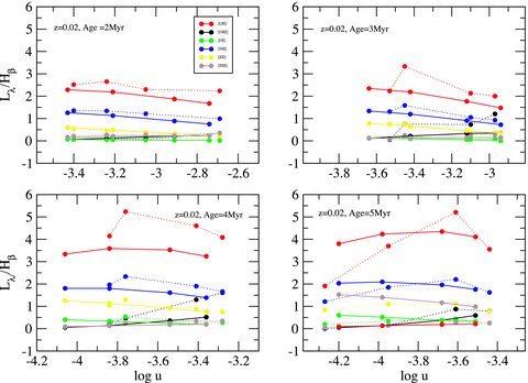
Evolution of emission lines at Z= 0.02 and SAL1 IMF for n_H= 10 cm⁻³ and log R (cm) = 20.84. Dotted lines correspond to old models by García-Vargas et al. (1995b) while solid lines correspond to new models.

Open in new tabDownload slide

We can see that, in general, the emission lines resulting from García-Vargas et al. (1995b) models are more intense than in the models computed in the present work for the same value of the ionization parameter. This is due to the use in the new set of models of NLTE blanketed atmosphere models for massive stars, which produce fewer hard ionizing photons. This new set of models explains in a natural way the emission-line ratios found in low-excitation high-metallicity H ii regions, as we will show in Section 4 and therefore do not require ad hoc explanations to keep the number of hard ionizing photons to the observed values.

3.3 Emission-line evolution

In this work, we follow the evolution of a given cluster during 5.2 Myr from their formation. After this time, in most cases and depending on metallicity, the gaseous emission lines are too weak to be measured due to the paucity of ionizing photons.

Figs 2(a)–(e) show the time evolution of the Hα luminosity and several emission-line ratios, as labelled, selected to represent the most relevant ionization stages of the most common elements: [O iii]λλ5007,4959/Hβ, [O ii]λ3727/Hβ, [O ii]λ3727/[O iii]λλ5007,4959, [O i]λ6300/Hα and [N ii]λ6584/Hα for models of different metallicity, computed with SAL2 IMF. In each figure, different colours correspond to a different cluster masses, from 0.12 × 10⁵ to 2 × 10⁵ M_⊙. The two different density cases, n_H= 10 and 100 cm⁻³, are represented by solid and dashed lines, respectively.

Open in new tabDownload slide

Open in new tabDownload slide

Open in new tabDownload slide

Figure 2

(a) Evolution of the Hα luminosity and five emission-line ratios for Z= 0.0001 (SAL2). The ratios are [O iii]λλ5007,4959/Hβ, [O ii]λ3727/Hβ, [O ii]/[O iii], [O i]λ6300/Hα and [N ii]λ6584/Hα. The more appropriate hydrogen recombination line has been chosen for normalization in order to minimize reddening effects. Solid lines correspond to models with n_H= 10 cm⁻³ while dotted lines correspond to models with n_H= 100 cm⁻³. Black, red, green, blue, yellow, brown and grey lines correspond to different cluster masses: 0.12, 0.20, 0.40, 0.60, 1.00, 1.50 and 2.00 ×10⁵ M_⊙, respectively. (b) Evolution of emission lines for Z= 0.0004 (SAL2). (c) Evolution of emission lines for Z= 0.004 (SAL2). (d) Evolution of emission lines for Z= 0.008 (SAL2). (e) Evolution of emission lines for Z= 0.02 (SAL2). Different colours and line code have the same meaning as in Fig. 2(a) for all of them.

For the lowest abundance models (Z < 0.0001), emission-line ratios involving oxygen lines are very weak (note the different scale in each metallicity panel) and its evolution is smooth. For intermediate-metallicity cases, the emission lines are intense, increasing with cluster mass.

In the first Myr of the evolution, the [O iii]]λλ5007,4959 lines are intense and then they decrease to rise again at 3–4 Myr, due to the presence of WR stars, that makes the equivalent effective temperature of the cluster become higher and causes an increase of the excitation during a short time. The appearance of the WR features and their duration depend on the mass and metallicity of the cluster as discussed in Paper I. The [O ii]λ3727 line shows moderate variations with metallicity. The [O ii]/Hβ ratio increases after 3 Myr of the star formation, being almost constant for low-metallicity models, before this age. As a result, the [O ii]/[O iii] ratio is very low for all metallicities at ages younger than 4 Myr. The oxygen emission lines are most intense for models with Z= 0.004. We will come back to the oxygen line evolution in the next section, when studying the diagnostic diagrams.

The low ionization line [O i]λ6300 is an indicator of the presence of strong winds and supernovae (Stasińska & Leitherer 1996) and, therefore, a burst age indicator. On the sole basis of the photoionization models, the intensity of this line increases with cluster age and [O/H] abundance; therefore, it shows higher values in old, evolved and high-metallicity H ii regions. The addition of shock contributions (not included in our models) would render this value even higher.

Finally, the [N ii]λ6584/Hα line-intensity ratio, which is in principle a good metallicity indicator, increases with increasing metallicity, even for regions with metallicities higher than Z= 0.004.

We have also produced photoionization models for ages older than 5.2 Myr (until 10 Myr) for the lowest metallicity cases, Z= 0.0001 and 0.0004 (see Fig. 3). The lower the metallicity, the hotter the zero-age main-sequence (ZAMS) and the longer the time spent by stars in the ZAMS. Hence, for the lowest metallicity clusters (Z= 0.0001 and 0.0004) we have explored the evolution further, to 10 Myr. However, the ionization parameters obtained are low, producing very weak (and sometimes undetectable) emission lines from high-ionization stages, like [O iii], specially for the lowest masses. Of course, these regions do exist and produce a low ionization spectrum, with observable [O i], [O ii] and [N ii] lines but negligible [O iii] line intensities which place them out of the plotted area of the diagnostic diagrams used in this work. Figs 4 and 5 illustrate this fact showing the results of the photoionization models for the 10 Myr evolution of an ionizing cluster of 1 × 10⁵ M_⊙ and a density of n_H= 10 cm⁻³ for two metallicities: Z= 0.0001 and 0.0004.

Figure 3

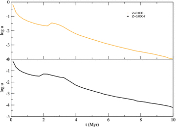
The ionization parameter as a function of age (beyond 5.2 Myr) for a 1 × 10⁵ M_⊙ cluster for low metallicities (Z= 0.0001 and 0.0004) and n_H= 10 cm⁻³.

Open in new tabDownload slide

Figure 4

Extended evolution (up to 10 Myr) of the Hα luminosity and five emission-line ratios: [O iii]λλ5007,4959/Hβ, [O ii]λ3727/Hβ, [O ii]/[O iii], [O i]λ6300/Hα and [N ii]λ6584/Hα, for a 1 × 10⁵ M_⊙ cluster, with Z= 0.0001 (SAL2) and n_H= 10 cm⁻³.

Open in new tabDownload slide

Figure 5

Extended evolution (up to 10 Myr) of the Hα luminosity and five emission-line ratios: [O iii]]λλ5007,4959/Hβ, [O ii]λ3727/Hβ, [O ii]/[O iii], [O i]λ6300/Hα and [N ii]λ6584/Hα, for a 1 × 10⁵ M_⊙ cluster, with Z= 0.0004 (SAL2) and n_H= 10 cm⁻³.

Open in new tabDownload slide

Figs 6 and 7 show the resulting sulphur emission-line ratios: [S ii]λλ6717,31/Hα and [S ii]λλ6717,31/[S iii]λλ9069,9532, as a function of the burst age. Sulphur line ratios were proposed as ionization parameter indicator by Díaz et al. (1991) and calibrations based on photoionization models at different metallicities were presented in Díaz et al. (2000) and Díaz & Pérez-Montero (2000). We have carried out a recalibration of this parameter using the models presented here that is given in details in Appendix A. Since the ionization parameter is directly related to the stellar cluster age, as suggested by García-Vargas et al. (1995a), we propose to use these sulphur lines as age indicators for H ii regions. Fig. 6 shows the [S ii]λλ6717,31/Hα ratio for the lowest metallicities (Z= 0.0001 and 0.0004) and all masses. Models with different values of n_H have been plotted in different panels. For a given metallicity, the plot shows that the line ratios involving the sulphur lines are low and rather constant during the first 3 Myr of evolution. From 3 to 5 Myr, they increase smoothly with age for all cluster masses. The line ratios also increase with cluster mass at a given age but cluster mass can be constrained via the derived number of ionizing photons from Balmer line luminosities.

Figure 6

The [S ii]λλ6717,31/Hα line ratio versus age (in Myr) for low metallicities (Z= 0.0001 and 0.0004) and all masses. Solid lines join models with Z= 0.0001 while dotted lines join models with Z= 0.0004. Different colours correspond to different values of the cluster mass. Models with values of n_H= 10 cm⁻³ have been plotted in the upper panel while models with n_H= 100 cm⁻³ have been plotted in the lower one.

Open in new tabDownload slide

Figure 7

The [S ii]λλ6717,31/[S iii]λλ9069,9532 line ratio versus age (in Myr) for high metallicities (Z= 0.004, 0.008, 0.02) and all masses. Solid lines join models with Z= 0.004, dotted lines those with Z= 0.008 and dashed lines those with Z= 0.02. Different colours correspond to different values of the cluster mass. Models with values of n_H= 10 cm⁻³ have been plotted in the upper panel while models with n_H= 100 cm⁻³ have been plotted in the lower one.

Open in new tabDownload slide

3.4 Emission-line intensities and the ionization parameter

Figs 8(a)–(e) show the intensity, with respect to Hβ of the following emission lines: [O ii]λ3727, [O iii]λ5007, [O i]λ6300, [N ii]λ6584, [S ii]λ6731, [S iii]λ9069 versus log u, obtained from the computed models, for metallicities Z= 0.0001, 0.0004, 0.004, 0.008 and 0.02. In each figure, four panels are shown for ages of 2 (top-left), 3 (top-right), 4 (bottom-left) and 5 Myr (bottom-right). Solid lines correspond to n_H= 10 cm⁻³ models while dotted lines correspond to n_H= 100 cm⁻³. In total, seven points per line are shown corresponding to seven values of the cluster mass: 0.12, 0.20, 0.40, 0.60, 1.00, 1.50 and 2.00 × 10⁵ M_⊙. We can see in the figures that models with n_H= 10 and 100 cm⁻³ follow the same trend, and cover different ranges of the ionization parameter value, with this being higher, as expected, for the lower density case.

Open in new tabDownload slide

Open in new tabDownload slide

Open in new tabDownload slide

Figure 8

(a) Evolution of emission-line intensities, as labelled, normalized to the Hβ intensity for Z= 0.0001 (SAL2) models as a function of the logarithm of the ionization parameter. Solid lines correspond to models with n_H= 10 cm⁻³ and dotted lines correspond to models with n_H= 100 cm⁻³. (b) Same as Fig. 8(a) but for Z= 0.0004. (c) Same as Fig. 8(a) but for Z= 0.004. (d) Same as Fig. 8(a) but for Z= 0.008. (e) Same as Fig. 8(a) but for Z= 0.02.

For a given metallicity, the changes in the emission-line spectrum and in the ionization parameter are due to the changes in the cluster mass, which determines the number of ionizing photons, and in the cluster age, which influences not only the total number of ionizing photons but also the overall ionization spectrum hardness and the ionized region size. For example, the [O iii]λ5007 line is intense during the first few Myr of the cluster evolution, for all metallicities, and then it decreases, to rise again at 4 Myr due to the presence of WR stars that produces a harder ionizing continuum.

From our models, we predict an intrinsic sizing effect in the H ii region evolutionary sequence, which implies a natural decreasing of the ionization parameter. For a very young region whose ionization is dominated by the O−B stars, the size is still small but the number of ionizing photons is high, resulting in a high ionization parameter. As the cluster evolves, the region size increases due to the stellar winds, but the number of ionizing photons decreases only slightly producing a decreasing ionization parameter, and therefore lower intensity lines. For the highest metallicities, this effect is more remarkable. High-metallicity regions have less ionizing photons and more intense winds therefore implying a lower ionization parameter. In addition, the effective cooling of the gas is transferred from the optical emission lines to the near and mid-infrared ones as metallicity increases. These two facts explain the fact that in high-metallicity regions, the optical emission lines are extremely weak, reaching in most cases only about one per cent of the Hβ line intensity. These lines are difficult to detect and this fact has biased the observational samples during a long time towards regions of a restricted metallicity range which has important implications for the interpretation of photometric samples of H ii regions.

4 DISCUSSION

4.1 Observational data

We have used first a compilation of data on H ii galaxies, high- and low-metallicity H ii regions and circumnuclear star-forming regions (CNSFR), with emission-line intensities measured for both the auroral and nebular [S iii] lines at λ 6312 and λλ 9069,9532 respectively. The data for CNSFR can be found in Díaz et al. (2007) where the appropriate references for the rest of the objects in the compilation can also be found. For all the regions, the electron density has been derived using the [S ii] ratio (Osterbrock 1989).

For this sample, metallicities have been derived following standard techniques in the cases in which electron temperatures could be derived. Otherwise, an empirical calibration based on the S₂₃/O₂₃ parameter (see Díaz et al. 2007) has been used.

Data from Castellanos et al. (2002a) correspond to H ii regions in the spiral galaxies: NGC628, NGC925, NGC1232 and NGC1637. The H ii regions have been splitted by density, which was derived from the [S ii] ratio. For seven regions, ion-weighted temperatures from optical forbidden auroral to nebular line ratios were obtained, and for six of them oxygen abundances were derived using empirical calibration methods. For the rest of the regions, metallicities have been estimated from the S₂₃ calibration (Pérez-Montero et al. 2006) and tailored photoionization models.

García-Vargas et al. (1997) give data of four H ii giant circumnuclear regions of NGC 7714. As usual, densities were derived from the [S ii] lines. Oxygen abundances were obtained by the electron temperature method thanks to the direct detection of the [O iii]λ4363 line.

Zaritski, Kennicutt & Huchra (1994) made an analysis of 159 H ii regions in 14 spiral galaxies, from which we have chosen those that have well-measured [S ii]]λλ6717,31 and [S iii]]λλ9069,9532 emission lines to obtain the density and the oxygen abundance through the S₂₃ parameter (Pérez-Montero et al. 2006). This reduces the number of H ii regions to 36.

We have also taken data from van Zee & Haynes (2006), corresponding to 67 H ii regions in 21 dwarf Irregular (dIrr) galaxies. They provide the emission-line intensities of the [O ii]λ3727, [O iii]λλ5007,4959 and [S ii]λλ6717,31 lines. In addition, they also provide the [S ii] line ratio, which we have used to derive the electron density. The [O iii] lines have been used to obtain the electronic temperature and consequently the oxygen abundance.

Data from Izotov & Thuan (2004) consist of H ii regions in 76 blue compact dwarfs (BCD) galaxies whose abundances have been derived using electron temperature from the ratio of the nebular to auroral [O iii] lines. All the regions of this sample have oxygen abundances lower than 12 + log(O/H) = 8.5. Data have been separated by density by means of the [S ii] line ratio.

Finally, Yin et al. (2007) provide data for 531 galaxies and H ii regions from the Sloan Digital Sky Survey Data Release 4 sample, from which the [O iii]λ4363 line has been measured and the oxygen abundances have been derived by standard methods. These data do not include the [S ii] lines and hence no electron density could be derived. The different observational data sources and the method used to derive the oxygen abundances are summarized in Table 3.

4.2 Diagnostic Diagrams: optical emission-line ratios

We have plotted together the model results and the observational data in different diagnostic diagrams in Figs 9–12. These diagrams can be used to study the relationship among different emission-line ratio and to extract information about the physical parameters of the ionizing clusters.

Figure 9

Diagnostic diagram showing log([O iii]λλ5007,4959,/Hβ) versus log([O ii]λ3727/Hβ) for models computed with SAL2 IMF. Each panel shows models for a different metallicity and the corresponding observational data in that metallicity range. Observational data come from: Zaritski et al. (1994) (circles), Izotov & Thuan (2004) (squares), Castellanos, Díaz & Tenorio-Tagle (2002b) (diamonds), van Zee & Haynes (2006) (triangles up), García-Vargas et al. (1997) (red triangles down) and Díaz et al. (2007) (asterisks of different colours: black: CNSFR; green: high-metallicity H ii regions; brown: low-metallicity H ii regions; magenta: H ii galaxies). Filled symbols represent objects with n_H= 100 cm⁻³, while open symbols have n_H= 10 cm⁻³, for data whose density has been obtained from the [S ii] ratio.

Open in new tabDownload slide

Figure 10

Diagnostic diagram showing log([O iii]λλ5007,4959/Hβ) versus log([O ii]λ3727/[O iii]λλ5007,4959) for models computed with SAL2 IMF. Each panel shows a different metallicity model and the corresponding data in that metallicity range. Symbols have the same meaning as in Fig. 9.

Open in new tabDownload slide

Figure 11

Diagnostic diagram showing log([O iii]λλ5007,4959/Hβ) versus log([N ii]λ6584/[O ii]λ3727) for models computed with SAL2 IMF. Each panel shows a different metallicity model and the corresponding data in that metallicity range. Symbols have the same meaning as in Fig. 9, with the addition of the blue dots, which correspond to H ii regions from Yin et al. (2007).

Open in new tabDownload slide

Figure 12

Diagnostic diagram showing log([O iii]λλ5007,4959/Hβ) versus log([N ii]λ6584/Hα) for models computed with SAL2 IMF. Each shell shows a different metallicity model and the corresponding data in that metallicity range. Symbols have the same meaning as that in Fig. 9 with the addition of blue dots which correspond to H ii regions from Yin et al. (2007).

Open in new tabDownload slide

Each figure is divided in four panels, one per metallicity: Z= 0.0001 and 0.0004 (top-left panel), 0.004 (top-right panel), 0.008 (bottom-left panel) and 0.02 (bottom-right panel). The highest metallicity value of the grid, Z= 0.05, has been excluded due to the absence of spectroscopic data with those high abundances. The lowest metallicity model tracks are plotted in the same panel as those corresponding to Z= 0.0004 to compare the position in the diagram of the emission lines of such low metallicities. Solid and dotted lines represent models with n_H= 10 and 100 cm⁻³, respectively. In each panel, the model metallicity is the central value of the different ranges, except for ranges 1 and 4 that include data with metallicities lower than Z= 0.0004 and higher than Z= 0.02, respectively. Different line tracks correspond to the evolution of the models with different cluster masses, from the lowest one on the right to the highest on the left. The observational data, taken from different sources as explained in the previous section, whose derived metallicities are in the range of the models we want to compare with, are shown in each panel. They have been divided by density and subdivided by metallicity according to the ranges given in Table 4.

The H ii regions plotted here describe a well-defined sequence in diagnostic diagrams which involve oxygen line ratios, like log([O iii]/Hβ) versus log([O ii]/Hβ) and log([O iii]/Hβ) versus log([O ii]/[O iii]) (Figs 9 and 10). Most of the observed regions are located in the panels corresponding to Z= 0.004 and 0.008 since few data exist for very low or oversolar metallicities. In fact, this is a bias effect since most popular H ii regions have been detected and catalogued through their high intensities of the [O iii]λλ5007,4959 lines, which happen in medium-low metallicity. Furthermore, it is at these metallicities, Z= 0.004 and 0.008, that a direct measurement of the [O iii]λ4363 line, used to derive the oxygen abundance, is possible.

Models of Z= 0.0001, 0.0004 and 0.02 do not have the aim of reproducing exactly the observation sequence but should be understood as metallicity limits for the observed regions. Observational data in these panels correspond to regions with metallicities lower than 12+log(O/H) = 7.7, in the first panel (upper-left), or higher than 12+log(O/H) = 8.7 in the last panel (bottom-right), as summarized in Table 4.

There are no observational data with Z < 0.0004. These regions have very low values of the [O iii]λ4363 line, undetectable with moderate size telescopes and standard signal-to-noise ratio values, and therefore their abundances have not been derived.

Our models predict that very low-metallicity regions have small sizes in Hα images where most of these H ii regions are catalogued and therefore observational samples can be seriously biased towards medium to large size H ii regions with metallicities Z > 0.001 (see Section 4.4 and Fig. 14 for a detailed discussion). For high metallicities, the [O iii]λ4363 line is not strong enough to be detected at a level of T_e determination and abundances have been derived through alternative methods as already described.

Figure 14

Evolution of the [O iii]λ4363/Hβ ratio for each metallicity, cluster masses from 0.12 to 1 × 10 ⁵ M_⊙ and n_H= 10 cm⁻³.

Open in new tabDownload slide

Our models cover the observational data range corresponding to different cluster masses. Different masses imply different numbers of ionizing photons and hence different values of the ionization parameter. These values decrease with time as the clusters evolve. The models involving the most massive stellar clusters have the highest ionization parameters, due to their higher number of ionizing photons at a given age. Less massive clusters follow a similar time evolution to the most massive ones, but starting at a lower initial value.

As explained before, regions with intense [O iii]λλ5007,4959/Hβ line ratios correspond to the highest ionization stages. For a given cluster mass, as the cluster evolves, the high-excitation emission lines tend to decrease while [O ii]/Hβ increases. This is due to the change of the ionization parameter with cluster evolution. For a very young region, whose ionization is dominated by O−B stars which produce a great amount of ionizing photons, the size is still small, and the resulting ionization parameter is high. As the cluster evolves, the region size increases due to the stellar winds while the number of ionizing photons remains almost constant (or even decreases) with respect to early phases. This effect makes the ionization parameter, hence the emission-line intensities and in particular the oxygen lines, to decrease.

This evolution influences also the data sample since early ages result in more compact regions (therefore high surface brightness) with high ionization parameters. Thus, the emission-line intensities of the [O iii]λλ5007,4959 lines are higher, increasing their detectability in a given sample obtained with the same instrumental configuration. In fact, most of the derived ages for those regions would be younger than 5 Myr, when they emit enough ionizing photons to produce a detectable Hα luminosity and from those, most of them would be biased towards younger ages (less than 3.5 Myr).

In Figs 9–13, there are no observations found in the tail of our models with high [O ii]λ3727 and low [O iii]λλ5007,4959 intensities. These values imply very low ionization parameters, that indicates more diffuse regions with low excitation. Since in most samples only the brightest H ii regions have been selected, due to their conspicuous Hα emission or their high values of the [O iii]λλ5007,4959 line intensities the lowest excitation regions tend to be excluded. Some of these regions could also be older low-metallicity regions (in the age range from 5 to 10 Myr, see Figs 4 and 5).

Figure 13

Diagnostic diagram showing log([S ii]λλ6717,6731/Hα) versus log([O iii]λλ5007,4959/Hβ) for models computed with SAL2 IMF. Each shell shows a different metallicity model and the corresponding data in that metallicity range. Symbols have the same meaning as in Fig. 9.

Open in new tabDownload slide

The influence of the electron density, although of second order, should also be considered. The models with n_H= 100 cm⁻³ show lower values of the ionization parameter. However, the radiation has more particles per cm⁻³ to ionize, and the excitation degree is higher, producing model sequences shifted upwards from the lower density ones. More significant differences between models of different densities are found in the highest metallicity diagrams (Z= 0.02).

4.3 Sulphur and nitrogen emission-line ratios

Diagnostic diagrams involving log([N ii]λ6584/Hα) and log([S ii]λλ6717,31/Hα) ratios have the advantage of using lines very close in wavelength, and therefore virtually reddening-free.

In large star-forming regions, like starbursts galaxies, the relationship between the excitation parameter [O iii]λλ5007,4959/Hβ and the metallicity indicator [N ii]λ6584/Hα gives us information about the youngest populations plus the star formation rate (Kennicutt, Tamblyn & Congdon 1994). At the beginning of the evolution, Hα emission is intense and comes from the ionizing photons produced by the most massive stars, most of them still in the main sequence. This number of ionizing photons increases with the cluster mass and decreases with metallicity. As the galaxy evolves, the Hα emission line decreases, while the [N ii]λ6584 line increases because of the gas ejection by stars.

The [N ii]λ6584/[O ii]λ3727 ratio was introduced as a good metallicity indicator by Dopita et al. (2000). Nitrogen is a secondary element, or, at least, it has a strong secondary component, which makes the ratio [N ii]/[O ii] to increase with metallicity. Besides, the value of the mean temperature of H ii regions decreases as metallicity increases. When metallicity rises, the electron temperature becomes too low to excite the O⁺ transitions; hence, [O ii] decreases while [N ii] does not, thus increasing the [N ii]/[O ii] ratio. A good correlation has been found between [N ii]/[O ii] and the N⁺/O⁺ ionic abundance ratio, which is assumed to trace the N/O ratio (Pérez-Montero & Díaz 2005). Also, Díaz et al. (2007) have shown that a very tight correlation between [N ii]/[O ii] and N/O exists for high-metallicity H ii regions and CNSFR, which follow a sequence of increasing N/O ratio with increasing emission-line ratio.

In our diagnostic diagrams of Fig. 12, we can see how this ratio changes with metallicity. For low-metallicity models, both the [O iii]/Hβ ratio and [N ii]/[O ii] ratio are low. As metallicity increases, both line ratios also increase. When metallicity reaches the limit of Z= 0.004, [O iii] starts to decrease while [N ii]/[O ii] ratio is still growing. At Z= 0.02, the models show low values of [O iii] and high values of [N ii]. The only available observational data in this part of the plot are high-metallicity H ii regions and CNSFR, showing high values of [N ii]/[O ii], which indicate high N/O abundance ratios, as can be seen in the sequence of Díaz et al. (2007).

Regarding the nitrogen abundance, it is well known that N is mainly primary for low metallicities and it is always possible to scale the N abundance that we include as input in cloudy by using a given function, such as the one obtained by Mollá et al. (2006) for the relationship of N/O versus O/H. However, we remark that in the models presented in this paper, we use SSP models where chemical evolution has not been taken into account, either for N or for the other elements as Fe or Ca. The nitrogen abundance has been scaled to the solar value as it has been done for the rest of the elements. Each element has its own evolution and in order to take this into account it is necessary to make precise calculations following a consistent method. This method can be seen in our previous works (Martín-Manjón et al. 2008; Martín-Manjón 2009) where we present photoionization models that use as input abundances the results obtained from chemical evolution models.

Finally, Fig. 13 shows the [S ii]λλ6717,31/Hα ratio versus [O iii]λλ5007,4959/Hβ also as almost reddening-independent. We can see that high values of the [S ii]λλ6717,31 line imply a low ionization parameter, and therefore a low [O iii] emission-line intensity. However, the [O iii]λλ5007,4959 lines are very metallicity-dependent, and a low intensity of this emission line could be due to a high metallicity rather than a low ionization parameter produced by an evolved population. Although both ratios are indicators of the ionization parameter, the values of u derived from oxygen emission-line ratios can be lower than the values of u derived from sulphur emission-line ratios, which are not so metallicity-dependent.

4.4 Abundance determinations in H ii regions and model consistency

Emission lines allow the determination of abundances by a direct method based on the electronic temperature, T_e, derived from suitable emission lines from which those of [O iii] are the most popular. We have obtained oxygen abundances from the modelled emission lines in order to check which is the most effective method to recover the oxygen abundance used as input for the models. An accurate analysis requires the detection of the auroral line [O iii]λ4363 with an intensity larger than 5 per cent of Hβ.

Fig. 14 shows the evolution of the [O iii]λ4363/Hβ ratio for each metallicity, n_H= 10 and for cluster masses of 0.12, 0.20,0.4, 0.6 and 1×10⁵ M_⊙. This ratio is high for Z= 0.0004 and 0.004, close to 5 per cent of Hβ in the first Myr of the evolution. However, for both, Z= 0.0001 and 0.008, [O iii]λ4363/Hβ has comparable values and below standard detection limits. Thus, the non-detection of this line can indicate either a high metallicity or a low oxygen content. For Z= 0.02, there is no [O iii]λ4363 line produced for this density case.

Fig. 15 shows the comparison between model oxygen abundances and the ones obtained by empirical methods. It can be seen that, from our photoionization models, we obtain the auroral line [O iii]λ4363 along the whole cluster evolution for metallicities in the range 0.0001 < Z < 0.008. The [O iii] line electron temperature method gives good results for all of them, with differences lower than 0.05 dex between input and derived abundances.

Figure 15

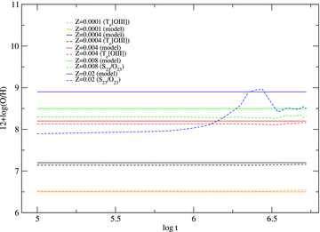
Comparison between abundances used as input for the models (solid lines) of different metallicities and abundances obtained using different empirical calibrators (dashed lines).

Open in new tabDownload slide

At Z= 0.008, corresponding to an oxygen abundance of 12+log(O/H) = 8.5, the [O iii]λ4363 line intensity range goes from 1.62 per cent of the Hβ intensity 1 Myr after the star formation, to 0.82 per cent 4 Myr after the burst. However, despite this line being detectable at this metallicity, the electronic temperature method is not able to reproduce the input metallicity of the model. Simple photoionization models are not able to reproduce the derived T_e in some situations. Stasińska (1978, 2002, 2005) showed that for high-metallicity H ii region models, the oxygen abundance derived from predicted emission-line ratios and the T_e method is lower than the one used as input in the models. These differences may be significant when large temperature gradients or fluctuations are present. In these cases, the temperature obtained from the emission line, T_l[O iii], is different from that derived from the [O iii] line ratio, T_r, and from the average ionic temperature T(O⁺⁺), with T_l[O iii] and T_r obtained from the models not being the representative temperature of the high ionization O⁺⁺ zone. Fig. 16 shows a plot similar to fig. 1 of Stasińska (2005) comparing a sequence of model derived oxygen abundances as a function of the input values. In this diagram, we can see that both sets of values coincide for low metallicities; for metallicities around 8.6 however, deviations become notorious and for higher metallicities the deviations are much more significant.

Figure 16

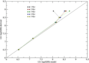
Comparison between abundances used as input for the models and abundances obtained using T_e-based methods. Each colour corresponds to a different age sequence. The values of 12+log(O/H) derived empirically are very close to the input values up to 8.6.

Open in new tabDownload slide

The abundances analysis in high-metallicity H ii regions is hampered by the fact that oxygen optical lines act as main coolant for the nebula; hence, a higher oxygen abundance leads to a more effective cooling. As the gas cools down, the electron temperature gets lower and the optical [O iii] forbidden lines get weaker. In general, this low excitation makes any temperature-sensitive lines in the optical range too weak to be measured. For this reason, empirical calibrators involving other lines besides the optical oxygen ones should be used (Pérez-Montero & Díaz 2005; Díaz et al. 2007). In our models, for metallicities Z= 0.008 and 0.02, abundances have been determined with the ratio S₂₃/O₂₃, obtaining reasonably good results for Z= 0.008 (with a difference of 0.2 dex approximately), but not for Z= 0.02, which shows important differences at the beginning of the evolution. For Z= 0.05, we cannot recover the oxygen abundance used as input by any empirical method since an effective calibration for such high-metallicity range (which is approximately 3 Z_⊙ in the reference system of Grevesse & Sauval 1998) has not been yet devised.

4.5 Ionized region equilibrium time and ionizing cluster age

The output of the photoionization models shows the picture of the ionized region once the equilibrium state is reached. This means that, when we observe an H ii region, what we really see is the effect of an ionizing cluster of a given age, regardless of the actual age of the ionized nebula. The time-step in our models corresponds to the stellar cluster age step given by the isochrone time resolution. The consequence is that the age resolution with which we can date the ionizing cluster from the information of the gas ionizing spectrum depends on the speed at which the nebula reaches the equilibrium, and this process is controlled by the metallicity. In the worst case, if the equilibrium time is longer than the cluster's age, it would be possible to see the effect of the ionizing cluster several Myr after the ionization. Therefore, the ionizing stellar cluster would be older than those inferred from the emission-line spectrum, being this observed cluster the result of its evolution during equilibrium time of the nebula. Wofford (2009) shows that the time it takes for an H ii region to reach thermal equilibrium at a metallicity of Z= 0.001 can be longer than 1 Myr within the first 5 Myr of evolution. The equilibrium time-scale increases with decreasing hydrogen density. In addition, it increases at lower metallicities, due to the low content of metals for cooling the gas.

We have tested this effect in our models by checking the equilibrium time in each cloudy model. Fig. 17 plots the age of the ionizing region given by cloudy once the equilibrium has been reached versus the age of the ionizing star cluster. Lines in orange, black, red and blue correspond to models with Z= 0.0001, 0.0004, 0.004 and 0.02, respectively. Solid lines refer to models for a cluster mass of 1 × 10⁵ M_⊙ while dotted lines to models for a cluster mass of 0.12 × 10⁵ M_⊙. All models have been computed with a density of n_H= 10 cm⁻³.

Figure 17

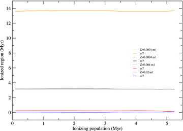
Relationship between the age of the ionizing stellar cluster and the recombination age of the ionized region. Orange, black, red and blue lines join models for Z= 0.0001, 0.0004, 0.004 and 0.02, respectively. Solid lines correspond to models for a cluster mass of up to 1 × 10 ⁵ M_⊙ while dotted lines correspond to a cluster mass of 0.12 × 10⁵ M_⊙.

Open in new tabDownload slide

A first conclusion to be extracted from this graph is that the age of the ionized region does neither depend on the cluster mass nor on the cluster age but it is controlled by the metallicity. This implies that neither the total number of ionizing photons nor the ionizing spectrum shape have a significant role in setting the equilibrium time of the ionized regions, which is controlled by the electron temperature (given by the metallicity). This is clearly seen in Fig. 17 where dotted and solid lines overlap and the ionized region age is almost constant along the cluster evolution. According to the computed models, the average equilibrium age is reached around t_eq= 13.6, 3.1, 0.2, 0.1 and 0.05 Myr for metallicities Z= 0.0001, 0.0004, 0.004, 0.008 and 0.02, respectively.

The second conclusion is that there are two metallicity regimes in which the ionizing cluster age has to be interpreted in a different way from the nebular emission-line spectrum. In moderate to high-metallicity H ii regions (Z≥ 0.004), the ionized nebula equilibrium time is shorter than the ionizing cluster age by a factor between 4 and 10. This means that for regions with metallicities above 0.004, we will derive the same age for the ionizing cluster whether we look directly to the embedded cluster (whenever possible) or we observe the cluster effects on the surrounding nebula, that is the nebular emission-line spectrum. In these cases, the resolution time, and therefore the error with which we can determine this age, is around 0.05 Myr at Z= 0.02, 0.1 Myr at Z= 0.008 and 0.2 Myr at Z= 0.004. In this metallicity regime, if we detect WR bumps in the optical spectrum or O, B and WR stars from UV images, we can assure, according to our results, that these stars are the ones responsible for the detected nebula ionization. On the contrary, in low-metallicity H ii regions, there is a delay between the time at which we observe the ionized region and the age of the stellar cluster responsible for this ionization. At Z= 0.0004, this delay is of the order of 3 Myr, which is consistent with the value of 1 Myr derived by Wofford (2009) for Z= 0.001. The delay can be as long as 13 Myr at Z= 0.0001. This implies that we may observe low-metallicity regions apparently ionized by a young cluster but without finding the expected young and hot stars when we observe directly inside the nebula. Moreover, we could find more evolved stars radiating in the IR as RSGs as the resulting products of the evolution of the ionizing stars. We suggest to take into account this result when interpreting the stellar content inside low-metallicity H ii regions.

4.6 Unveiling the physical properties of the ionizing clusters

The purpose of this piece of work is to show that it is possible to unveil the properties of the young cluster responsible for the ionization on the basis of the emission-line spectrum of the ionized gas alone. In what follows, we suggest some recommendations to find the physical properties of the dominant young ionizing population (see flow diagram in Fig. 18).

Figure 18

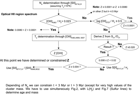
Flow diagram to unveil the ionizing cluster physical properties through the gas optical emission-line spectrum

Open in new tabDownload slide

1. The first parameter than can be determined is the electron density, which is derived from the [S ii]λλ6716, 6731 lines. This value influences the ionization parameter and therefore it is an important input for our models.

2. The metallicity can be derived or constrained once the electron density has been determined. If the value of [O iii]λ4363/Hβ is higher than 0.023, then abundances can be derived by standard methods using the electron temperature calculated from the [O iii]λ4363, [O iii]λ4959, [O iii]λ5007 line ratio. We remark that the absence (or a very low value) of optical [O iii] lines is an indicator of very low or very high metallicity. popstar includes models with metallicity as low as Z= 0.0001. If the value of [O iii]λ4363/Hβ is lower than 0.023, we recommend to check the value of log([O ii]λ3727/Hβ). Values lower than 0.5 indicate very low metallicities while the opposite indicates that the region is in the high-metallicity regime. In this latter case, we can estimate the metallicity through empirical methods (Pérez-Montero & Díaz 2005). These methods allow to estimate abundances up to solar values (Z= 0.02). Values higher than those are usually not found in optically selected samples since these regions are efficiently cooled by IR lines and have a very faint optical emission-line spectrum.

3. The age should be constrained once the metallicity evaluation has been carried out. We propose to use the diagnostics with [S ii]λλ6716,31/Hα (Fig. 6), for low-metallicity regions, and [S ii]λλ6716,31/[S iii]λλ6069,9532 (Fig. 7), for high-metallicity regions. In both cases, we need to use the electron density to select among different sets of models. We have computed models for two density values: 10 and 100 cm⁻³, which we recommend to use when electron density is less than 50 cm⁻³ or higher than 50 cm⁻³, respectively, and up to a maximum value of 400 cm⁻³. On the basis of these diagrams and the observed values of the line ratios, we can distinguish if the ionizing cluster is younger or older than 3 Myr. The resolution at which we can estimate the age depends on the equilibrium time as discussed in Section 4.5. In the case of low-metallicity regions (below Z= 0.004), the equilibrium time is of the order of, or even longer than, the ionizing cluster age. This has to be taken into account when observations of the embedded stars are available, since in this low-metallicity scenario these stars are the result of the evolution of the ionizing cluster and not the ionizing cluster itself.

4. The luminosity of Hα emission line is directly related to the number of ionizing photons, and therefore to the mass of the cluster. However, Hα luminosity depends not only on the cluster mass but also on the age and metallicity, even during the first 5 Myr of evolution (see Fig. 2) when the emission-line spectrum in the optical is detectable, according to our models. Moreover, Hα is detected up to an age of 20 Myr, when the emission-line spectrum is not yet detectable (we remind the reader that this paper is focused on the first few Myr when emission lines are prominent, since these are the regions available in most H ii region catalogues). Due to the former reasons, it is difficult to derive the mass without previous estimates of metallicity and age. Therefore, we propose to derive the mass of the cluster from the Hα luminosity (Fig. 2) using the previously found restrictions on metallicity and age.

5. Finally, we can use the values of the complete set of emission lines to check the consistency of our determination.

Since this process is too slow to be applied to a large sample of objects, we are developing a fast software tool, based on the previous guidelines and using minimization algorithms, to find the best model that fits the emission-line values and determine the physical properties of the young cluster responsible for the ionization of a given H ii region, when spectroscopic data are available.

5 SUMMARY AND CONCLUSIONS

We present a new grid of evolutionary models as a tool to estimate the mass, age and metallicity of the dominant ionizing stellar population of a given H ii region from its optical emission-line spectrum.

We provide a complete set of photoionization models for H ii regions along the first 5.2 Myr of their evolution, using as ionizing source a very young star cluster obtained from the theoretical evolutionary synthesis models popstar Paper I.3 The basic grid is composed of SSPs computed with different IMFs and a wide range of metallicities (Z= 0.0001, 0.0004, 0.004, 0.008, 0.02 and 0.05). A Salpeter IMF with m_low= 0.15 M_⊙ and m_up= 100 M_⊙ has been used in this work. The ionizing cluster is assumed to form in a single burst. Our grid considers five values of the total cluster mass (0.12, 0.20, 0.40, 0.60, 1.00, 1.50 and 2 × 10⁵ M_⊙), covering the range of observed H ii regions. As the cluster evolves, the stellar winds and supernovae blow the material, determining the H ii region size. This material is ionized by the emergent continua. We use the photoionization code cloudy to obtain the corresponding H ii region emission-line spectrum once the equilibrium is reached.

We present diagnostic diagrams where we compare our model results with a large sample of observed H ii regions, whose metallicities have been consistently computed in a homogeneous manner according to the most appropriate method for each metallicity range. It is found that, in general, our models can satisfactorily reproduce the observations.

Finally, we show that the emission-line spectrum from an ionized region provides a powerful tool to unveil the physical properties of the embedded young cluster responsible for the gas ionization and propose some guidelines to constrain its physical properties.

This work has been partially supported by DGICYT grant AYA2007–67965-C03-03 and partially funded by the Spanish MEC under the Consolider-Ingenio 2010 Program grant CSD2006-00070: First Science with the GTC (http://www.iac.es/consolider-ingenio-gtc/). Also, partial support from the Comunidad de Madrid under grant S-0505/ESP/000237 (ASTROCAM) is acknowledged. The authors thank an anonymous referee for valuable comments and suggestions that have contributed significantly to the quality of this paper.

REFERENCES

Appendix

APPENDIX A: IONIZATION PARAMETER RECALIBRATION

This appendix includes a re-calibration of the ionization parameter for high- and low-metallicity H ii regions with sulphur lines, as can be seen in Figs A1 and A2, respectively. As we have explained in the paper, we do not use the ionization parameter as an input for our models since we derive it from the physical properties of the ionizing clusters and the assumed geometry of the ionized nebula. However, since many other models use this magnitude to parametrize their grids or use different geometries for the ionized regions, we have considered it interesting to obtain a re-calibration of the relationship between the ionization parameter and the sulphur lines. We have used for that the results from our models, as a self-consistent set of values typical for H ii regions.

Figure A1

Calibration of the ionization parameter u from the [S ii]λλ6717,31/[S iii]λλ9069,9532 line ratio for high-metallicity models: Z= 0.004 (black dots), 0.008 (red dots), 0.02 (green dots), and two particle densities, n_H= 10 (upper panel) and 100 cm⁻³(lower panel). The calibration has been made for values of log u < − 2 and it is represented by orange dots.

Open in new tabDownload slide

Figure A2

Calibration of the ionization parameter u from the [S ii]/Hα line ratio for the models with metallicities Z= 0.0001 (black dots) and 0.0004 (red dots), and both densities n_H= 10 (upper panel) and 100 cm⁻³ (lower panel). The calibration is represented by orange dots.

Open in new tabDownload slide

The [S ii]λλ6717,31/[S iii]λλ9069,9532 line ratio has been shown to be a good ionization parameter indicator for moderate to high metallicities (Díaz et al. 1991), with little dependence on metallicity. García-Vargas et al. (1995a) proposed to use the ratio [S ii]/[S iii] to derive the ionization parameter of high-metallicity regions (Z > 0.004). We have re-calibrated this relationship for each model. This calibration has been made for values of the ionization parameter log u < − 2 since most H ii regions observational data do not show ionization parameters higher than this. For a more accurate calibration for higher ionization parameter values, a particular model, according to cluster mass, should be selected since a high dispersion in the model results for different masses is found.

For high-metallicity models, we find a cubic polynomial relationship between log u and log[S ii]/[S iii]. There are small differences between models of Z= 0.008 and 0.004 and models of Z= 0.02, which makes it necessary to provide two different equations for log u in order to obtain accurate calibrations.

For n_H= 10, we obtain log u=− 2.865 − 1.175x+ 0.139x²− 0.135x³ (Z= 0.008 and 0.004) log u=− 2.705 − 1.736x+ 0.698x²− 0.973x³ (Z= 0.02), where 6717,31/[S iii]λλ9069,9532).

For n_H= 100, we obtain log u=− 3.136 − 0.810x+ 0.685x²− 0.784x³ (Z= 0.008 and 0.004) log u=− 2.938 − 1.051x+ 0.043x²− 0.482x³ (Z= 0.02), where 9069,9532).