The velocity function of gas-rich galaxies Free

Abstract

1 INTRODUCTION

The galaxy luminosity function is one of the best-known tools for comparing theoretical models of galaxy formation with the observable Universe. Modern large-scale cosmological simulations, based on the hierarchical clustering of gravitationally interacting particles, need to reproduce the space density of galaxies seen in the observed luminosity function. However, in reality such a comparison is complicated because galaxy luminosities are not a direct output of these simulations. Galaxy luminosity is non-trivially linked to halo mass through poorly understood processes such as star formation efficiency, feedback and gas accretion. Recent semi-analytical models attempt to tie the N-body simulations to observable quantities by applying physically motivated or empirical recipes for star formation, gas accretion, AGN feedback etc. (e.g. Baugh et al. 2005; Bower et al. 2006; De Lucia & Blaizot 2007; Obreschkow et al. 2009). These models produce a range of measurable galaxy properties, such as luminosity in different bands, gas masses and star formation rates, and the distribution functions of these quantities can be tested against observations. Although such semi-analytical models are increasingly more successful in reproducing the observable universe (see review by Baugh 2006), the method inherently implies a very indirect way of comparing galaxy space densities. A much more direct test of the simulations can be made if the properties of simulated haloes are compared directly with observable quantities. Such a comparison is possible through the galaxy circular velocity function φ(V_c), which is defined as the number density of galaxies as a function of their rotational velocity.

The galaxy circular velocity traces the total dynamical mass of a galaxy, which is dominated by its dark matter content. Therefore, the measured velocity function should match that of dark haloes in simulations. However, it should be realized that baryons still potentially affect the comparison in two unrelated ways. First, for surveys to detect the galaxies and include them in samples that are used to create the velocity function, the galaxies need to have a minimal detectable number of baryons in the component and phase being searched for. Whether in an individual galaxy these baryons are primarily in cold gas, in old stars or in young stars may affect this galaxy's detectability. Secondly, baryon physics can significantly affect the density structure of dark matter haloes and consequently have an effect on its rotational velocity. Especially in the inner regions of galaxies, the baryonic component can contribute significantly to the rotational velocity and in some cases the baryons can dominate the dynamics in the central regions. Therefore, although the velocity function provides a much more direct tool to compare simulations and observations than galaxy luminosity functions, these two limitations should be kept in mind in making the comparison.

There have been a number of attempts in the past to construct the galaxy velocity function by using published luminosity functions and then converting these into velocity number density distributions using scaling relations such as the Tully–Fisher relation (for late-type galaxies) and the Faber–Jackson relation or the Fundamental Plane (for early-type galaxies). Shimasaku (1993) and Gonzalez et al. (2000) apply this method to an array of optical surveys and find consistent velocity functions (within a factor of 2), with a Schechter-like distribution, but with a steeper than exponential decline at the high velocities. As is stressed by Kochanek & White (2001) and demonstrated by Sheth et al. (2003), this simple conversion from a luminosity function via a scaling relation can lead to erroneous measurements of φ(V_c) if the scatter on the scaling relations is not taken into account. Kochanek & White (2001) mention a number of other systematic problems with this method of measuring φ(V_c), prime among which are the errors in morphological classification of galaxies and calibration of the magnitude scale. They put special effort in reducing these systematic uncertainties and measure a non-parametric φ(V_c). Sheth et al. (2003) measure φ(V_c) for early-type galaxies from the Sloan Digital Sky Survey (SDSS) taking full account of the scatter in the relation between luminosity and velocity, Chae (2010) takes a similar approach for SDSS and 2dF galaxies and Choi, Park & Vogeley (2007) use volume-limited SDSS subsamples to construct a velocity function for early types.

In this paper, we present the first measurement of the velocity function of late-type galaxies that is not dependent on scaling relations. We base this measurement on the H i Parkes All Sky Survey (HIPASS), a blind 21 cm emission-line survey covering the whole southern sky up to declination +25°. From the region south of declination +2°, a catalogue of 4315 H i-selected galaxies has been extracted as presented in Meyer et al. (2004) and Zwaan et al. (2004). The advantage of this large galaxy sample is that the velocity width W is one of the data products of the original survey data. Therefore, after doing the appropriate volume corrections and correcting the velocity widths for inclination, the velocity function can be measured directly without taking the step of measuring V_c separately or assuming a global scaling relation for all galaxies. The HIPASS catalogue is 99 per cent complete at a peak flux of 84 mJy and an integrated flux of 9.4 Jy km s⁻¹. This integrated flux limited translates to a minimal detectable H i mass of 5.5 × 10⁷ M_⊙ at a distance of 5 Mpc.

The paper is organized as follows. In Section 2 we present the galaxy sample we use in our analysis, summarize the method for calculating space densities and discuss the observed velocity width function. Velocity functions for late-type galaxies are presented and compared with previous inferred velocity functions in Section 3. We also discuss the contribution from early-type galaxies. In Section 4, we compare our results with those of recent Λ cold dark matter (ΛCDM) simulations. Section 5 discusses some observational biases that could affect the evaluation of the velocity function. Finally, we summarize our results in Section 6. For distance-dependent quantities, we use H₀= 70 km s⁻¹ Mpc ⁻¹ and define h₇₀=H₀/(70 km s⁻¹ Mpc ⁻¹) = 1.

2 THE HIPASS VELOCITY WIDTH FUNCTION

2.1 Calculating space densities

In Zwaan et al. (2003), we derived a bivariate stepwise maximum likelihood (2DSWML) technique, which solves for the space density of objects as a function of H i mass and velocity width simultaneously. We specifically designed this method for a peak-flux-limited sample, but in Zwaan et al. (2004) we demonstrated how the method can be adjusted to produce reliable space densities for samples constructed using different selection criteria. In that paper, we also showed how to use the 2DSWML technique to calculate for each galaxy individually an effective volume V_eff. These values are now the maximum likelihood equivalents of V_max for the standard Σ1/V_max method (Schmidt 1968), and summing the values of 1/V_eff in bins of H i mass gives the original 2DSWML solution for the H i mass function. The normalization of space densities is retained by equating the mean galaxy density to the integral over the H i mass function. After this normalization is applied to V_eff, these values represent true volumes. Any distribution function of a parameter measured for the HIPASS sample can now be determined by a binned summation of 1/V_eff. We refer to Zwaan et al. (2004) for a more detailed description of the method.

2.2 The velocity width function

We use the velocity widths W measured at 50 per cent of the peak flux density of the H i profile. In principle, for high signal-to-noise ratio data, the widths measured at 20 per cent of the peak flux density will provide more direct measurements of the full rotation, but we prefer the 50 per cent values because these latter values are less sensitive to noise in the 21 cm spectra. Meyer et al. (2008) have shown that the scatter in the Tully–Fisher relation is smaller when using 50 per cent measurements instead of those measured at 20 per cent. The observed linewidths are corrected to their rest-frame values (relativistic effect), instrumental broadening and turbulent motion, all according to standard procedures. A full description of the corrections applied to the observed velocity widths is described in Meyer et al. (2008). Henceforth, we refer to the velocity width corrected for instrumental and relativistic broadening as W. Note that for the calculation of rotational velocities, an additional correction for turbulent broadening is applied.

Fig. 1 plots the distribution function of H i profile widths, φ(W). This function can be readily calculated by summing 1/V_eff in bins of W. Error bars represent uncertainties in the measurements determined by quadratically summing 1/V_eff within each bin. This estimate gives an indication of the pure statistical uncertainty, which mostly ignores effects due to local large-scale structure. All 4315 HIPASS detections presented in Meyer et al. (2004) are represented in this diagram as no optical identifications are required for constructing this function. The error on W measurements is σ_W= 7.5 km s⁻¹, independent of the profile width (Zwaan et al. 2004).

Figure 1

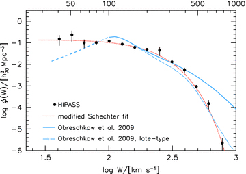
The space density of local gas-rich galaxies as a function of their observed profile widths corrected for relativistic broadening and instrumental broadening. The short-dashed line is a modified Schechter fit to the data points (see text). The solid line is the distribution function based on the Obreschkow et al. (2009) simulations, while the long-dashed line represents this sample limited to late-type galaxies only.

Open in new tabDownload slide

To provide a parametric description of this distribution, we fit it with a modified Schechter function of the form

1

where Γ is the gamma function. In the next section, we give a physical motivation for this parametrization of a velocity function. We find a good fit to the measured data points with the following values: φ_*= 0.67 h³₇₀ Mpc⁻³, log W_*/km s⁻¹= 2.21, α= 0.10 and β= 1.56.

Although no true physical parameter is represented in this diagram, it does present a straightforward comparison to simulated galaxy samples. Since it does not depend on cross-matching with optical catalogues, it shows the distribution function of observed profile widths of a purely H i-selected sample. This function is relevant for calculating the detection efficiency of future H i 21 cm surveys, as the ability to separate 21 cm signals from the noise is a strong function of profile width.

An interesting comparison is with the work of Obreschkow et al. (2009), who calculate cold gas properties for the semi-analytic galaxy catalogues of De Lucia & Blaizot (2007) based on the N-body simulations of CDM by Springel et al. (2005). Velocity widths are assigned to simulated galaxies by making assumptions on the rotation curves and gas distributions. We refer to Obreschkow et al. (2009) for details on how velocity widths are calculated. The solid line in Fig. 1 shows the distribution function of W from these simulations. Below W= 100 km s⁻¹, we draw a dashed line to indicate that the simulations are incomplete in that range due to the limited mass resolution. For the W measurements from Obreschkow et al. (2009), we used the raw W₅₀ values multiplied by sin i. In the range 100 km s⁻¹ < W < 400 km s⁻¹ the HIPASS points match the Obreschkow et al. (2009) points fairly well, although the simulations over-predict the space density of galaxies just above the mass resolution limit. Towards higher velocities the observations show an exponential decline, whereas the observations display a power-law distribution. Clearly, the simulations predict too many very broad profile (W > 400 km s⁻¹) galaxies compared to what HIPASS detected. The H i mass function of the Obreschkow et al. (2009) catalogue also shows an overproduction of very massive galaxies (their fig. 3), but the difference in our Fig. 1 is much larger. To investigate this discrepancy further, we also plot in the same figure the simulated distribution of late-type galaxies only and find that they match the observed distribution (without any morphological-type cut applied) much better. Therefore, it appears that the Obreschkow et al. (2009) simulations overproduce a population of gas-bearing massive early-type galaxies that is not observed in HIPASS.

3 A TYPE-DEPENDENT ROTATIONAL VELOCITY FUNCTION

3.1 A velocity function for late-type galaxies

The next step is to determine the distribution of true rotational velocities. We calculated these V_c values by applying an inclination correction to the projected velocity spread of the H i gas: V_c=W (2 sin i)⁻¹. Henceforth, we refer to the rotational velocity V_c as the velocity width corrected for turbulence, instrumental broadening, inclination and corrected to rest-frame profile widths, as detailed in Meyer et al. (2008). We note that V_c should be regarded as the velocity corresponding to the maximum of the rotation curve as this is essentially the velocity that is probed by integrated H i velocity profiles. In principle, more accurate measurements of galaxy halo masses could be achieved my making use of V_flat, the velocity corresponding to the flat part of the rotation curve, but high-resolution 21 cm synthesis observations are required to make such measurements. Verheijen (2001) discusses the use of V_c and V_flat in the Tully–Fisher relation and their relation to halo mass.

The required inclinations cannot be measured from the HIPASS data directly because the Parkes Telescope beam at 21 cm of 13 arcmin [full width at half-maximum (FWHM)] does not spatially resolve most galaxies. Doyle et al. (2005) searched for optical counterparts to the HIPASS detections and found unique optical identifications for 2646 (62 per cent) galaxies. For these galaxies, Doyle et al. (2005) list b_J-band axial ratios measured from the SuperCOSMOS data. Inclinations are calculated from the axial ratios q and corrected for internal thickness of the discs q₀ using the relation

2

where we adopt q₀= 0.2. It has been argued that q₀ should depend on galaxy morphology (Giovanelli et al. 1997), but we follow the recommendation of Tully et al. (2009) that a consistent use of q₀ is important for the avoidance of systematic errors. We note that Meyer et al. (2008) found that inclinations derived from the b_J measurements resulted in a lower Tully–Fisher scatter than those from the Two-Micron All-Sky Survey (2MASS) J-band measurement.

Selecting galaxies on the basis of their H i content naturally results in a sample weighted towards gas-rich galaxies. However, this does not imply that early-type galaxies (S0/E) are missing from the catalogue. In fact, some recent studies have shown that 70 per cent of early-type galaxies have detectable amounts of H i with masses exceeding a few times 10⁶ M_⊙ (e.g. Morganti et al. 2006; Oosterloo, Fraternali & Sancisi 2007). The H i morphologies range from small clouds to large, regular low column density discs. Furthermore, in Zwaan et al. (2003) we have measured the H i mass function of early-type galaxies, based on an initial sample of 1000 bright HIPASS galaxies, indicating that early types are present in 21 cm survey catalogues. However, in the analysis of the HIPASS data we wish to exclude the early-type galaxies for two reasons. First, even though a large fraction of early types has detectable H i, we are certainly missing a significant fraction of those early types that are gas free or sufficiently gas poor to be absent from the HIPASS sample. Secondly, H i measurements do not provide reliable velocity dispersions for early-type galaxies. As already stated, early-type H i morphologies are not predominantly ordered discs that trace the full potential of the galaxies. This fact is also supported by the observation that H i masses do not correlate with early-type luminosity or mass (Serra et al. 2008). Optical surveys such as the SDSS, completed with optical spectroscopy, are much better equipped to measure the distribution function of early-type velocity dispersions (Sheth et al. 2003; Choi et al. 2007; Chae 2010). To cull the early-type galaxies from the sample, we rely on the morphological classifications as listed by Doyle et al. (2005). This takes out 11 per cent of the galaxy sample.

We also exclude all galaxies with measured inclinations i < 45° to avoid introducing large uncertain inclination corrections that may affect the shape of the velocity function. This amounts to 30 per cent of the sample. To account for the excluded galaxies, the final velocity function is corrected with a factor 1/(1 −f) where f is the fraction of excluded galaxies.

In Fig. 2 the measured velocity function is shown as solid circles, whereas the open symbols indicate the effect of changing the inclination cut-off from 45° to 35° and 55°. The effect of changing the inclination cut-off is not noticeable for V_c above approximately 100 km s⁻¹, but at lower V_c the changing cut introduces some scatter. There is a weak trend of space densities dropping with a higher inclination cut, and increasing with a lower inclination cut, although the error bars are too large to make a conclusive statement: the mean space density of objects with V_c < 80 km s⁻¹ changes less than 1σ when the inclination cut is varied from 45° to 35° or 55°.

Figure 2

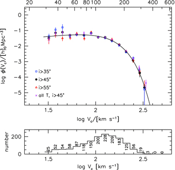
Top panel: the HIPASS late-type velocity function φ(V_c). The solid circles show φ(V_c) for morphological types Sa and later and inclinations i > 45°. The other symbols show the effects of choosing different inclination cut-offs and including early-type galaxies. The solid line represents the best-fitting modified Schechter function (see text). Bottom panel: histogram of rotational velocities for our sample of HIPASS galaxies with i > 45° and types Sa and later.

Open in new tabDownload slide

Also in Fig. 2, we show the effect of ignoring the morphological-type selection by plotting the velocity function for all morphological types. The effect is only detectable beyond V_c > 200 km s⁻¹, but even there early-type galaxies make a very minor contribution to the space densities.

Similar to the distribution function of W, we fit the rotational velocity function with a modified Schechter function of the form

3

where φ_* is the space density of galaxies near the ‘knee’ of the distribution, V_c* is the characteristic rotational velocity, α is the low-velocity power-law index and β is the high-velocity power-law index. The latter parameter β enters the equation when the traditional Schechter luminosity function is transformed to a velocity function using a relation between luminosity L and rotational velocity, e.g. the Tully–Fisher relation: L∝V^β_c. In reality, the value of β in the parametrized velocity function is not equal to the Tully–Fisher power law because the scatter in the Tully–Fisher relation affects the way in which the luminosity function is transformed to φ(V_c) and because the Tully–Fisher power law changes as a function of luminosity and morphological type. These effects have been described in detail by e.g. Sheth et al. (2003). A traditional Schechter function would provide a very poor fit to the measured velocity function because the high-end exponential drop-off does not decline fast enough to fit the data points. We find a satisfactory fit to the data with the following parameters: φ_*= (0.061 ± 0.027) h³₇₀ Mpc⁻³, log V_c*/km s⁻¹= 2.06 ± 0.09, α= 0.66 ± 0.47 and β= 2.10 ± 0.37. It should be noted that errors on individual parameters are very large because of the strong covariance between all fitting parameters. In particular, the dimensionless covariance between log V_c and β is r(log V_c, β) = 0.99 and that between φ_* and α is r(φ, α) =−0.97. The lowest covariance value is r(φ_*, β) = 0.78. By just fitting the low-velocity slope (V_c < 100 km s⁻¹) of the distribution, we find α=−0.90 ± 0.25.

Fig. 3 reproduces the HIPASS velocity function and compares our result with recent estimates of the late-type velocity function based on the 2dF and SDSS galaxy redshift surveys from Chae (2010). In that study, published luminosity functions were adopted for the SDSS late-type galaxies from Choi et al. (2007) and for 2dF from Croton et al. (2005). Next, they Monte Carlo simulate a large sample of galaxies, based on these luminosity functions and the Tully–Fisher relation, taking into account the intrinsic scatter. For the Tully–Fisher relation, the measurement by Pizagno et al. (2007) was adopted, which is based on Hα rotation curves of a sample of 162 SDSS galaxies. The velocity functions are found by summing the simulated galaxies in bins of V_c. In Fig. 3, the upper dashed curve shows the result based on the 2dF luminosity function and the lower dashed curve is based on the SDSS. Discrepancies between the two functions are indicative of the systematic errors introduced by converting galaxy luminosities between different wave bands that are used in the luminosity function and Tully–Fisher relation measurements, different definitions of morphological type (based on spectroscopy or colour), and differences in the 2dF and SDSS galaxy luminosity functions (as discussed in e.g. Liske et al. 2003).

Figure 3

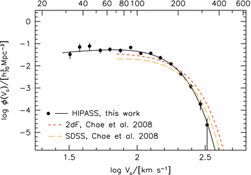
The HIPASS late-type velocity function φ(V_c) as indicated by the circles with error bars. The solid curve is a modified Schechter function fit. The two dashed curves show the late-type velocity function based on the 2dF data (upper curve) and SDSS data (lower curve) as calculated by Chae (2010).

Open in new tabDownload slide

Given the very different galaxy samples and methods for calculating the velocity function, we find reasonable agreement between the directly measured HIPASS velocity function and the inferred 2dF and SDSS velocity functions. At lower velocities, we find slightly higher space densities compared to the indirect measurements and at higher velocities we find slightly lower values. The most significant difference between our measurement and previous estimates is that we can determine the space densities of galaxies down to much lower values of V_c: the HIPASS velocity function goes down to V_c≈ 30 km s⁻¹, whereas the previous measurements only reach V_c≈ 70 km s⁻¹. The measured velocity function is remarkably ‘flat’ (power-law slope ≈−1) down to the lowest rotational velocities.

3.2 The contribution from early-type galaxies

Because 21 cm emission is not a good tracer of the gravitational potential of early-type galaxies, we have so far excluded these galaxies from our analysis. It would, however, be interesting to derive the total local universe velocity function of all galaxy types. To put early- and late-type galaxies on the same V_c scale, we adopt a conversion from velocity dispersion σ to rotational velocity: ⁠. This conversion is based on the assumption that the mass distribution of an elliptical galaxy can be modelled as a singular isothermal sphere. Desai et al. (2004) test this assumption using literature measurements of velocity dispersion and optical circular velocities in the flat regions of the rotation curves and find V_c≈ 1.54σ, illustrating the uncertainty in estimating V_c values for early types.

The most recent estimates of early-type velocity functions are those by Chae (2010), based on 2dF and SDSS using a method similar to that described for the late-type galaxies. Fig. 4 shows these measurements as indicated by a shaded thick curve, of which the upper boundary corresponds to the calculation based on 2dF data and the lower boundary corresponds to the SDSS. Other recent calculations of the SDSS velocity function have been presented by Sheth et al. (2003) and Choi et al. (2007), the latter being based on direct measurements of velocity dispersions. However, this study may suffer from incompleteness at low-velocity dispersions. As shown by Chae (2010), the different space density measurements of early-type galaxies around the peak of the distribution (V_c≈ 300 km s⁻¹) agree very well, but below that point the slopes of φ(V_c) vary between the different studies. Issues with completeness, related to both incomplete dispersion measurements and missing low luminosity early types, are probably causing the discrepancies. See also Mitchell et al. (2005) for a discussion on inferred and measured early-type velocity functions.

Figure 4

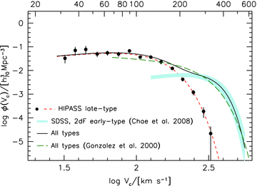
The points with error bars show the HIPASS late-type velocity function with a modified Schechter function fit indicated by a short-dashed line. The shaded curve represents the early-type velocity function derived from 2dF data (upper boundary) and SDSS data (lower boundary) as estimated by Chae (2010). The solid curve is the summed velocity function for all morphological types. The Gonzalez et al. (2000) all-types result is represented by a long-dashed line. Late-type galaxies dominate the statistics below V_c≈ 200 km s⁻¹.

Open in new tabDownload slide

The solid curve in Fig. 4 shows the summed velocity function for all morphological types, adding the HIPASS late-type curve and the 2dF/SDSS-based early-type curve of Chae (2010). For comparison, we also show the velocity function from Gonzalez et al. (2000) based on Southern Sky Redshift Survey 2 (SSRS2) data. Their result is in good agreement with later calculations by Kochanek & White (2001), although these authors do not give a parametrized description of their velocity function. The overall consistency between the HIPASS plus 2dF/SDSS velocity function with the earlier work of Gonzalez et al. (2000) is reassuring. Again, HIPASS adds important data points at the low V_c end of the velocity function.

Fig. 4 illustrates that the galaxy velocity function is dominated by late-type galaxies below V_c≈ 200 km s⁻¹, whereas early-type galaxies take over above that point. It should be noted that the early-type measurements are based on samples having relatively high luminosity cut-offs. Dwarf elliptical (dE) galaxies are therefore largely missing from the analysis. In field regions, late-type spirals and irregular (Irr) galaxies dominate the space densities at the low-mass end. This is both apparent from optical surveys (Binggeli, Sandage & Tammann 1988) and H i surveys (Zwaan et al. 2003). Dwarf ellipticals only become significant contributors to the space density in cluster environments. The evidence from H i mass function studies is that 21 cm surveys fully recover the faint-end slope of the luminosity function (Zwaan, Briggs & Sprayberry 2001). Therefore, the contribution from gas-less early-type dwarfs is marginal in the volume sampled by HIPASS. Desai et al. (2004) construct velocity functions for cluster galaxies and find that their function is steeper than that in the field, which is also attributed to a contribution of low-mass early-type galaxies, which are relatively scarce in a large volume of space.

4 COMPARISON WITH THEORY

The CDM model of galaxy formation with a cosmological constant Λ makes robust predictions for the mass function of dark matter haloes. Cosmological simulations determine the mass function slope with high accuracy, giving ψ(M) ∝M^−1.9 (e.g. Sheth, Mo & Tormen 2001; Sheth & Tormen 2002; Giocoli, Tormen & van den Bosch 2008; Tinker et al. 2008; Boylan-Kolchin et al. 2009). To convert this function into the distribution function of individual galaxies, halo occupation distribution (HOD) has to be applied (Peacock & Smith 2000; Cooray & Sheth 2002). The number density of galaxies may be higher than that of dark matter haloes since each dark matter halo can contain a number of galaxies.

ΛCDM models generally predict that the total dynamical galaxy mass M_dyn relates to rotational velocity V_c as M_dyn∝V^β_c. In our definition of rotational velocity, V_c is comparable to the maximum rotational velocity, for which definition Bullock et al. (2001) found that β≈ 3.4. Applying this conversion to the power-law mass function slope of α_M=−1.9, we can estimate the power-law slope α of the velocity function

4

5

6

finding that the power-law slope of φ(V_c) should be approximately α=−4.0. Of course, this simple estimate ignores many subtleties of HOD and baryon physics, but does illustrate that theory probably predicts a low-V_c slope much steeper than α≈−1, which we find for the HIPASS velocity function.

The clearest manifestation of this problem with ΛCDM is the so-called substructure problem: around the Milky Way galaxy ΛCDM predict hundreds of low-mass satellites, although only an order of magnitude fewer objects are detected (Klypin et al. 1999; Moore et al. 1999). Recent surveys identify a growing number of satellites around the Galaxy and M31 (see Zucker et al. 2006; Ibata et al. 2007, for some examples), but still not in sufficient quantities to alleviate the problem. By accounting for baryonic physics, Simon & Geha (2007) manage to reduce the missing fraction of satellites to approximately a factor of 3, but baryon physics are extremely complicated and uncertain in these dense environments to the extent that reconciliation between theory and observations is presently too model dependent. We note, however, that Koposov et al. (2009) demonstrate that models with a constant stellar mass fraction and strong suppression of star formation before reionization in haloes with V_c < 10 km s⁻¹ can produce the observed satellite counts.

The range of masses that we are probing with HIPASS is clearly higher than that of the Milky Way satellites. H i-selected galaxy samples are inherently composed of fairly isolated systems as 21 cm surveys are not very efficient in probing high density regions (Waugh et al. 2002). The galaxies that we probe in the tail of the velocity function are predominantly dwarf Irr galaxies and low-mass spirals (cf. Zwaan et al. 2003).

To make a direct comparison with simulations, we need a V_c distribution function of dark matter haloes. Blanton, Geha & West (2008) compare an inferred velocity function of isolated dwarf galaxies with isolated haloes in the N-body, pure dark matter simulations of Kravtsov et al. (2004). Due to the first-order similarity of the observed data sets, we also use this Kravtsov-based sample as our dark matter halo reference distribution.

Unfortunately, Blanton et al. (2008) present cumulative distribution functions of V_c, which make quantitative comparisons very difficult. We differentiate their cumulative distribution function of dark matter haloes to derive φ(V_c) and show the result in Fig. 5 as a dotted line. Interestingly, the space densities calculated from simulations and HIPASS match very well in the range 100 km s⁻¹ < V_c < 200 km s⁻¹. To some level, this is a coincidence because the definition of isolation for the dark matter haloes is not matched to that of the HIPASS catalogue. Blanton et al. (2008) show that the space densities in this V_c range increase somewhat if a more relaxed definition of isolation is applied. Of more significance is the marked difference in the slope of the velocity function below V_c≈ 100 km s⁻¹, where the simulations predict a slope of α≈− 3, compared to our observation of α≈−1. Simulations clearly predict many more haloes than are detected by HIPASS.

Figure 5

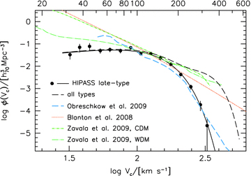
The HIPASS velocity function (filled circles with solid line) compared with the velocity function from a selection of simulations. The blue dashed line shows the simulations of Obreschkow et al. (2009) for late-type galaxies. The green short dash–dotted and long dash–dotted lines are the CDM and WDM simulations from Zavala et al. (2009) for all galaxy types, respectively. For comparison, the observed velocity function for all galaxy types from Fig. 4 is reproduced as the black dashed line. The red dotted line shows the dark matter haloes from Blanton et al. (2008).

Open in new tabDownload slide

There is one important caveat in this comparison, which is the mass resolution of the cosmological simulation. The (Kravtsov et al. 2004) simulations, used by Blanton et al. (2008) to calculate velocity functions, reliably determine space densities of haloes down to V_c≈ 70 km s⁻¹. Below that value, we have used the power-law extrapolation of Blanton et al. (2008).

Another interesting comparison with our observations is that with the recent results of Obreschkow et al. (2009). These authors have reprocessed the semi-analytic simulations of De Lucia & Blaizot (2007), which, in turn, are based on the ‘millennium run’, a CDM N-body simulation of a (714 Mpc/h₇₀)³ volume, containing 3 × 10⁷ galaxies. Obreschkow et al. (2009) use a set of physical prescriptions to assign H i and molecular hydrogen (H₂) to these galaxies and are able to reproduce many of the observed gas properties of local galaxies. The simulated H i mass function is well matched to the one measured from HIPASS for H i masses in excess of M_{H I}≈ 2 × 10⁸ M_⊙. The scatter in the observed and simulated M_{H I}–W₅₀ relation is very large (their fig. 13), but this M_{H I} limit approximately translates into a rotational velocity limit of V_c≈ 100 km s⁻¹, implying that space densities of galaxies below V_c≈ 100 km s⁻¹ are not reliably predicted.

To estimate V_c values from the Obreschkow et al. (2009) catalogue, we use their measurements of w^peak_{H I}, which is the linewidth between the two peaks of the double-horned H i profile. We use V_c= (w^peak_{H I}+ 12)/2 to derive rotational velocities, where the correction of 12 km s⁻¹ is applied to correct for profile smoothing due to the velocity dispersion of the gas. That is, w^peak_{H I} slightly underestimates the true V_c as can be seen in fig. 11 of Obreschkow et al. (2009).

The thick dashed line in Fig. 5 shows the resulting velocity function, plotting the result for late-type galaxies to enable a direct comparison with the HIPASS results. The agreement in the shape of φ(V_c) above V_c≈ 100 km s⁻¹ is striking; only above V_c= 300 km s⁻¹ do the simulations over-predict the observed number density. Unfortunately, at the low velocity end we cannot make a detailed comparison because the mass resolution of the millennium run is not sufficiently high to predict space densities in this regime.

Higher resolution simulations are available from the recent work of Zavala et al. (2009). These authors use constrained CDM and warm dark matter (WDM) simulations of a (29 h⁻¹₇₀ Mpc)³ volume centred around the Local Group. The WDM simulations are based on a power spectrum using a fitting function that approximates the transfer function for a thermal WDM particle with m_WDM= 1 keV. Their velocity functions are reproduced by short dash–dotted and long dash–dotted lines for CDM and WDM, respectively. Although their simulations assume that all galaxies are disc galaxies, they do not differentiate specifically between early- or late-type galaxies. We reproduce the velocity function for all galaxy types from Fig. 4 as a long dashed line to compare the Zavala et al. (2009) results with. The simulated curves are purported to be complete above V_c= 35 km s⁻¹. Zavala et al. (2009) also test the effect of supernova feedback on the shape of the velocity function and conclude that it only marginally reduces the space densities at the low V_c end.

For a comparison with their simulations, Zavala et al. (2009) use preliminary results from the Arecibo Legacy Fast ALFA survey (ALFALFA; Giovanelli et al. 2005), concentrating on publicly released data bases in the Virgo direction region (Giovanelli et al. 2007) and the anti-Virgo direction region (Saintonge et al. 2008). In total, the comparison is based on a small sample of 201 galaxies, 186 of which are in a high density region and the remaining 15 in a low density region. Only galaxies out to a distance of 29 h⁻¹₇₀ Mpc are considered. Since the preliminary ALFALFA results are based on a much smaller galaxy sample, probing a smaller volume than HIPASS, and concentrate only on a clear overdensity and an underdensity, we do not attempt to make a direct comparison with our results. We note, however, that the shape of the ALFALFA φ(V_c) as presented by Zavala et al. (2009) is qualitatively in good agreement with our results.

Comparing our HIPASS measurements with the Zavala et al. (2009) simulations, we essentially reach similar conclusions: above V_c= 100 km s⁻¹, the CDM predictions are in good agreement with the observations. Below V_c= 100 km s⁻¹, CDM clearly predicts too many low-mass haloes. Similar to the Blanton et al. (2008) results, CDM predicts a steep low-velocity slope as estimated by equation (6). The WDM simulations predict a fairly flat velocity function, in much better agreement with the observations.

5 BIASES

In making comparisons between our HIPASS results and simulations, there are a number of biases that should be discussed here. First, an important issue is whether the 21 cm velocity widths truly probe the full range of the galaxy velocity curve. If the detectable H i is confined to the central regions of the galaxies, the H i rotation curve might not measure the full rotational velocity of the dark matter halo (e.g. Swaters et al. 2009). Inspecting the dwarf galaxy rotation curves of Swaters et al. (2009), it can be seen that most galaxies do just reach a flat part, but there are notable exceptions, especially those with rotational velocities lower than V_c≈ 60 km s⁻¹. This implies that a fraction of our lower V_c measurements probably underestimates the true rotational velocity of the dark matter haloes. As an extreme test, we randomly multiply half our V_c measurements below 60 km s⁻¹ with a factor of 1.5 and construct φ(V_c) using this new estimate. Fig. 6 shows the result, where filled symbols show the original space densities and open circles represent those after making the correction. Not surprisingly, the space density of objects with V_c just below 90 km s⁻¹ is boosted after making the correction. In effect, the discrepancy between ΛCDM theory and our observations is slightly reduced just below the knee of the distribution, but not significantly at lower V_c. The effect that the space density drops below 50 km s⁻¹ is a result of the fact that many V_c below that value shift to higher V_c bins, but no very low-velocity systems replace them because they do not exist in our sample.

Figure 6

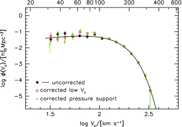
Testing the effect of possible biases on the shape of the rotational velocity function. The solid circles and line show the velocity function as presented in Fig. 2. The open circles demonstrate the effect of increasing the rotational velocity of low-mass galaxies for which the flat part of the rotation curve might not be reached. The open triangles show how the velocity function changes if velocity widths are corrected for pressure support.

Open in new tabDownload slide

A second concern is whether gas velocity dispersions in low-mass galaxies should be taken into account in calculating rotational velocities that measure the full potential. In very low-mass galaxies, the gas velocity dispersions can be comparable in magnitude to the measured rotational velocities, adding a significant pressure support term compared to rotational support. If H i synthesis maps are available, asymmetric drift correction can be made that corrects for the pressure support. Begum et al. (2008a,b) study a sample of very low-mass galaxies with rotational velocities as low as 10 km s⁻¹. For each galaxy individually, they correct for pressure support and find significant corrections to V_c. We find that their corrections can be fitted as ΔV_c= 130/V_c, which we can apply to our data to make a rough correction for pressure support. The triangles in Fig. 5 show combined effect of this correction and the correction described in the previous paragraph. We find that the pressure correction has no measurable effect on φ(V_c).

Finally, we discuss how much cosmic variance can affect our measurements. In Fig. 7 we display the velocity function for four different quadrants of the southern sky. For each quadrant, we simply use the Σ1/V_eff method as described in Section 2, where the V_eff values are the maximum likelihood equivalents of the effective search volumes for each galaxy, calculated from the complete HIPASS sample. Also shown are the least-squares-modified Schechter fits to each set of data points. Although the variation between the data points for the different quadrants is approximately a factor of 2 at the high V_c end and even larger at the low V_c tail, the fitted functions show good consistency between the quadrants. The only deviant velocity function is that of the fourth quadrant, which is clearly an underdense region. Despite a factor of 2 lower overall normalization, the shape of the velocity function of the fourth quadrant is not significantly different from those of the other three quadrants. We conclude that our main result that the low V_c slope of the velocity function is ‘flat’ is unchanged if we subdivide our sample into smaller regions on the sky. Cosmic variance in the HIPASS survey volume is discussed in more detail in Zwaan et al. (2003).

Figure 7

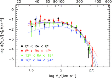
The effect of cosmic variance on the circular velocity function. The four different symbols show the velocity function for four different quadrants of the southern sky and dotted lines show modified Schechter fits. The solid line represents the fit to the full HIPASS sample.

Open in new tabDownload slide

6 SUMMARY AND DISCUSSION

We have used the HIPASS sample of H i-selected galaxies to calculate the circular velocity function φ(V_c) of late-type galaxies. Optical identifications of the HIPASS galaxies were used to determine inclinations and morphological types. Our determination of the rotational velocity function is the first that uses a direct method, where the same galaxy sample is used for measurements of V_c and the evaluation of space densities. Previous estimates of the φ(V_c) were dependent on a conversion of the galaxy luminosity function and a relation between luminosity and rotational velocity (the Tully–Fisher relation). In these analyses, different data sets were used for the calculation of the luminosity function and the Tully–Fisher relation.

We find good agreement between our velocity function and inferred velocity function from the literature, but we are able to measure space densities down to V_c= 30 km s⁻¹, a factor of 2 lower than previous estimates. A standard Schechter function is not a good fit to φ(V_c) because space densities decline too rapidly at high velocities compared to an exponential drop-off. Instead, we use a modified Schechter function, which provides an excellent fit to the data points. In order to find a velocity function for all galaxy types, we add the early-type measurements from Chae (2010).

As stated in Section 1, the velocity function is one of the most direct tests of galaxy formation models. Our velocity function is compared with those derived from ΛCDM galaxy formation simulations, and we find a good agreement in the space density of objects with circular velocities V_c > 100 km s⁻¹. Below this value ΛCDM predicts too many objects, reaching a discrepancy of a factor of 20 at V_c= 30 km s⁻¹. WDM simulations are constructed to reduce the power on small scales and hence produce velocity functions with a flatter low-end slope, which provide a better fit to our data points. Primack (2009) argues that observational limits on the mass of the WDM particle are already very strict. The circular velocity function essentially tests cosmological models on scales of approximately 1 Mpc (Blanton et al. 2008). Similar scales are probed by the Lyα forest power spectrum, and it is found that the mass of the WDM particle should be more than 4 keV (Viel et al. 2008) (or more than 1.7 keV according to a more recent analysis by Boyarsky et al. 2009).

Blanton et al. (2008) use a sample of 12 low-mass-isolated dwarf galaxies and an independent measurement of the luminosity function to compare with ΛCDM predictions and claim consistency down to V_c≈ 50 km s⁻¹. Our analysis, and also that of Zavala et al. (2009), indicates that the inconsistency between observations and simulations is significant over a larger range in velocities, up to V_c≈ 100 km s⁻¹. We argue that our constraints are firmer than those of Blanton et al. (2008) because our HIPASS measurement is based on ∼50 times more galaxies below V_c= 100 km s⁻¹ and is not reliant on optical luminosity functions.

Apart from adopting WDM, which other factors could be responsible for the mismatch between observed and simulated rotational velocity functions? In Section 5 we tested whether observational biases, such as dwarf galaxy rotation curves not probing the full potential or ignoring pressure terms, could have an effect on φ(V_c) and concluded that the effect was insignificant. There are, however, astrophysical effects that could conceivably affect the shape of the measured φ(V_c).

Our analysis is based on the assumption that low-mass galaxies contain a detectable amount of neutral gas. Any gas-free low-mass field galaxies would escape inclusion in the HIPASS sample. Geha et al. (2006) obtained Green Bank Telescope 21 cm observations of 101 low-mass field galaxies and detected H i emission in 88 per cent of those. It therefore seems unlikely that many low-mass systems are missing from our analysis. A correction to the low V_c end of a factor of 1/0.88 would not change the slope significantly.

UV background photoionization of primordial gas could impact the formation of low-mass objects (e.g. Babul & Rees 1992; Efstathiou 1992). Recent calculations do not reach consistent conclusions on the magnitude of this effect and the characteristic V_c below which the effect becomes important. For example, variations in the reionization history, the inclusion of self-shielding in the calculations and the link with SN feedback all have important effects (e.g. Susa & Umemura 2004; Hoeft et al. 2006; Mesinger & Dijkstra 2008; Pawlik & Schaye 2009; Sawala, Scannapieco & White 2009, and references therein). At present, it remains unclear whether the suppression of low-mass system formation by the UV background is sufficient to explain the observed local velocity function. Similarly, the effect of SN feedback might be important. SN feedback implies chemical enrichment, heating and entraining of surrounding gas, and reducing the gas fractions of low-mass systems (e.g. Dekel & Silk 1986; White & Frenk 1991). The treatment of SN feedback in simulations of galaxy formation is very complicated and, like UV photoionization, the importance of the effect is still a topic of discussion (Scannapieco et al. 2006). It should be noted though that Zavala et al. (2009) conclude that the SN feedback has only a minor effect on the z= 0 circular velocity function.

Future blind H i surveys with instruments such as the Australian SKA Pathfinder (ASKAP) will probe much larger volumes than HIPASS with a lower noise level and much higher spatial resolution. For instance, a 1 year survey covering 75 per cent of the sky will find approximately 5 × 10⁵ galaxies, 3 × 10⁴ of which will be spatially resolved, thus allowing the measurement of rotation curves and hence of more accurate rotational velocities. This, in combination with the much larger number of galaxies, a higher sensitivity to low-mass galaxies and the ability to study different environments, will allow much more accurate measurements of the galaxy rotational velocity function in the local universe.

MAZ acknowledges the hospitality of the University of Western Australia in Perth where most of this work was carried out. We thank the anonymous referee for a detailed and constructive report. The Parkes telescope is part of the Australia Telescope which is funded by the Commonwealth of Australia for operation as a National Facility managed by CSIRO.

REFERENCES