


Abstract
We explore the properties of the Hβ emission line profile in a large, homogeneous and bright sample of N∼ 470 low-redshift quasars extracted from Sloan Digital Sky Survey (Data Release 5). We approach the investigation from two complementary directions: composite/median spectra and a set of line diagnostic measures (asymmetry index, centroid shift and kurtosis) in individual quasars. The project is developed and presented in the framework of the so-called 4D Eigenvector 1 (4DE1) parameter space, with a focus on its optical dimensions, full width at half-maximum of broad Hβ[FWHM(Hβ)] and the relative strength of optical Fe ii[RFe ii≡ W(Fe ii4434–4684 Å)/W(Hβ)]. We reenforce the conclusion that not all quasars are alike and spectroscopically they do not distribute randomly about an average typical optical spectrum. Our results give further support to the concept of two populations A and B [narrower and broader than 4000 km s−1 FWHM(Hβ), respectively] that emerged in the context of 4DE1 space. The broad Hβ profiles in composite spectra of Population A sources are best described by a Lorentzian and in Population B by a double Gaussian model. Moreover, high- and low-accretion sources (an alternative view of the Population A/B concept) not only show significant differences in terms of black hole (BH) and Eddington ratio Lbol/LEdd, but they also show distinct properties in terms of line asymmetry, shift and shapes. We finally suggest that a potential refinement of the 4DE1 space can be provided by separating two populations of quasars at RFe ii∼ 0.50 rather than at FWHM(Hβ) = 4000 km s−1. Concomitantly, the asymmetry and centroid shift profile measures at 1/4 fractional intensity can be reasonable surrogates for the FWHM(Hβ) dimension of the current 4DE1.
1 INTRODUCTION
1.1 Current view on the structure of broad-line region of AGN
1.1.1 Observational considerations
A defining characteristic of type 1 active galactic nuclei (AGN) is the presence of broad emission lines in their optical and ultraviolet (UV) spectra. We cannot resolve the AGN central regions at other than radio (Very Long Baseline Interferometry – milliarcsecond resolution) or, more recently, infrared (IR; e.g. Raban et al. 2009) wavelengths. This leaves the structure, geometry, kinematics and nebular physics of the broad line region (BLR) beyond our direct reach. It is unlikely that we will spatially resolve the central regions of more than a few low-z AGN in the foreseeable future. We are left with two practical methods to probe the BLR structure and kinematics: (a) reverberation studies (e.g. Koratkar & Gaskell 1991; Peterson 1993; Peterson & Wandel 1999; Wandel, Peterson & Malkan 1999; Kaspi et al. 2000; Peterson et al. 2004; Kaspi et al. 2007; Bentz et al. 2009) and (b) single epoch spectroscopy for large numbers of sources. The former requires dedicated spectroscopic monitoring to achieve temporal resolution of a relatively small number of sources while the latter provides kinematic resolution for multitudes of sources. The time lag between line and continuum flux variations (in the former approach) provides an estimate of the BLR size. A few dozen (mostly low z) sources have been monitored with typical BLR radii in the range from a few light-days to several light-weeks (e.g. Peterson 1993; Kaspi et al. 2000; Bentz et al. 2009). Spectroscopy of large samples provides a much-needed empirical clarification since, without a clear understanding of the phenomenology, one can build models filled with misconceptions about BLR structure/geometry, kinematics and nebular physics.
We have been exploring the phenomenology of quasars in the context of a 4D Eigenvector 1 parameter space (4DE1; Sulentic, Marziani & Dultzin-Hacyan 2000a; Sulentic et al. 2000b; Marziani et al. 2001, 2003a,b; Sulentic et al. 2007), which serves as a spectroscopic unifier/discriminator for all type 1 AGN. We take it as self-evident that such a parameter space is needed: (1) to emphasize source differences, (2) to help remove the degeneracy between the spectroscopic signatures of orientation and physics and (3) to provide a context within which to interpret results of multiwavelength studies of individual sources. We adopted four principal 4DE1 parameters because they were relatively easy to measure in large numbers of sources and because they showed large intrinsic dispersion and sometimes major differences between subtypes. The principal parameters involve measures of: (i) full width at half-maximum of broad Hβ[FWHM(Hβ)], (ii) equivalent width ratio of optical Fe ii (λ4570 Å blend) and broad Hβ, RFe ii= W(FeIIλ4570 Å)/W(Hβ), (iii) the soft X-ray photon index (Γsoft) and (iv) C ivλ1549 Å broad-line profile velocity displacement at half-maximum, c(1/2). Various lines of evidence (Sulentic et al. 2007) suggested a change of source properties near FWHM(Hβ) = 4000 km s−1, which motivated the introduction of the Population A–B distinction in order to emphasize the differences. This is similar to the radio-quiet (RQ) versus radio loud (RL) distinction, but appears to be more effective (Sulentic et al. 2007; see also below).
Previous studies (Sulentic et al. 2003; Zamfir, Sulentic & Marziani 2008) indicate that RL sources show a much more restricted 4DE1 domain space occupation [FWHM(Hβ) versus RFe ii] than the RQ majority (∼78 per cent of all RL quasars belong to Population B domain and ∼62 per cent of RQ belong to Population A domain). This was in part the motivation for our Population A–B distinction. A majority (≈55–60 per cent) of quasars show broad Balmer lines with FWHM(Hβ) < 4000 km s−1 (Sulentic et al. 2000a,b; Zamfir et al. 2008) and are labelled Population A. Population A shows: (1) a scarcity of RL sources (3–4 per cent at most; Zamfir et al. 2008), (2) strong/moderate Fe ii emission, (3) a soft X-ray excess (perhaps the consequence of a high-accretion rate; e.g. Wang & Netzer 2003), (4) high-ionization broad lines (HIL; e.g. C ivλ1549Å) showing blueshift/asymmetry and (5) low-ionization broad line profiles (LIL) best described by Lorentz fits (Sulentic et al. 2002; Bachev et al. 2004; Sulentic et al. 2007; Marziani et al. 2009).
Population B sources: (1) include the large majority of the RL sources: ∼91 per cent of all Fanaroff–Riley II (FR ii) and ∼62 per cent of all core-dominated RL quasars or, alternatively, ∼17 per cent of all Population B sources are RL quasars (and this is a conservative1 estimate; see Zamfir et al. 2008), (2) show weak/moderate Fe ii emission, (3) do not show a soft X-ray excess, (4) do not show HIL blueshift/asymmetry and (5) show LIL Balmer lines best fit with double Gaussian models (Sulentic et al. 2002; Bachev et al. 2004; Sulentic et al. 2007; Marziani et al. 2009). Fundamental differences between the BLR in Population A and B sources (and between RL and RQ quasars) appear to be lower electron density (e.g. Collin-Souffrin 1987; Collin-Souffrin, Hameury & Joly 1988a) in Population B along with a less flattened cloud distribution (e.g. Zheng, Sulentic & Binette 1990; Sulentic et al. 2000a; Collin et al. 2006). Some of the Population B sources with very broad LIL profiles show double-peaked structure (e.g. Eracleous & Halpern 1994), but they are rare. None the less, there is an underlying idea that a double-peaked signature is hidden in most profiles. Murray & Chiang (1997) have emphasized that a disc+wind model favours the regions of low projected velocity in the disc, which leads to a predominance of single-peaked profiles. The existence of double-peaked profiles is not a necessary condition to prove the reality of a disc BLR geometry (e.g. Popović et al. 2004, and references therein).
Valuable insights are provided by studies of emission lines of different ionization levels: HIL, e.g. C ivλ1549 Å and LIL, e.g. Balmer lines, Fe ii, Mg ii doublet λ2800 Å. The HIL and LIL are probably produced in distinct regions (e.g. Collin-Souffrin et al. 1988b) at least in Population A sources as inferred from the difference in the time delayed response to continuum variations (see section 4.1 of Sulentic et al. 2000a). While C iv is always broader than Hβ (produced at smaller radii?) in Population A sources, the two lines tend to scale more closely or, in some cases, Hβ tends to show broader profiles (Sulentic et al. 2007) in Population B.
There has been a great deal of disagreement over the meaning of often poor spectroscopic data for often small samples. Making progress involves a lot of work obtaining spectra with good signal-to-noise (S/N) and resolution in order to assemble representative sample. Ideally, one would like be able to observe the same line(s) over a large redshift range, which raises obvious difficulties that infrared spectroscopy has begun to alleviate (e.g. Sulentic et al. 2004, 2006; Marziani et al. 2009, and references therein). Or, even better, observe concomitantly both HIL and LIL for the same source with awareness that the BLR in high- and low-luminosity sources may be different as well (Netzer 2003; Kaspi et al. 2007; Netzer & Trakhtenbrot 2007; Marziani et al. 2009).
We suggest that the best hope of advancing our understanding of the AGN phenomenon lies with better empiricism, which is the path to model improvement. The first step to progress requires a reasonably large (i.e. representative) quasar sample for which uniform and good quality spectra exist. We argue that progress cannot come from studies of indiscriminately averaged quasar spectra, whether their S/N is high or low. This statement is false only if all quasars are virtually identical, which we know to not be true.
There is a long series of questions in need of answers. Do RQ and RL quasars show the same geometry/kinematics? Do optical/UV spectra offer predictive power on the likelihood of a source being or becoming RL? How many broad line emitting regions exist in a source and is it the same number in all sources? Can we distinguish high- and low-accretors spectroscopically? How are broad and narrow emission lines related geometrically and kinematically? How much variance in nebular physics exists from source to source? Do quasars change spectroscopically from low to high redshift?
1.1.2 Geometrical and kinematical inferences
Current best guesses about geometry and kinematics involves the idea that all or much of the broad-line emission arises from a flattened cloud distribution (possibly an accretion disc) and that kinematics are dominated by Keplerian motions. (e.g. Peterson & Wandel 1999, 2000). There are empirical arguments in favour of a flattened geometry, which pertain mostly to RL quasars. An observed anticorrelation between the width of the Balmer lines (FWHM) and the core:lobe radio flux density ratio R (Wills & Browne 1986) or equivalent alternatives (Wills & Brotherton 1995; Corbin 1997) can be explained by observation of a flattened BLR at different viewing angles. Similar conclusions could be drawn from an analysis of the FWHM as a function of radio spectral index α (Jarvis & McLure 2006) or the Balmer decrement as a function of R (Jackson & Browne 1991). In superluminal quasars, the viewing angle θ can be determined with good accuracy and there are reported correlations between θ or other beaming indicators and Balmer lines FWHM (Rokaki et al. 2003; Sulentic et al. 2003) that favour an axisymmetric BLR dominated by rotation. Zamfir et al. (2008) find that FR ii (Fanaroff & Riley 1974) quasars show both broader Hβ profiles (ΔFWHM ≈ 2000 km s−1) and weaker Fe ii (ΔRFe ii≈ 0.2) than the core/core-jet RL quasars.
Collin et al. (2006) offer arguments that inclination effects are apparent only in sources with narrow profiles – what we call Population A. Studies in the 4DE1 context suggest that kinematics and geometry are very different for Population B sources. Even if RL quasars of Population B show correlations consistent with a flattened geometry the BLR, it must be different than the one suggested for narrow-line Seyfert 1 (NLSy1; Osterbrock & Pogge 1985) and other Population A sources; for example if only for the simple reason that the minimum FWHM observed in face-on RL quasars is at about 3000 km s−1 broader than the narrowest Population A Balmer profiles ∼500–600 km s−1, whose flattened BLR is also assumed observed face-on (e.g. Zhou et al. 2006; Zamfir et al. 2008). The assumption of Keplerian motion in the BLR [and of FWHM(Hβ) as a virial estimator] finds support from the discovery that the minimum observed FWHM(Hβ) increases systematically with source luminosity [from ≈1000 km s−1 at log Lbol(erg s−1) = 44 to ≈3000 km s−1 at log Lbol(erg s−1) = 48]. This trend is easily explained if we are observing line emission from a Keplerian disc obeying a Kaspi (Kaspi et al. 2000, 2007) relation (Marziani et al. 2009).
1.2 The drivers of type 1 AGN diversity
Numerous studies sought to explain the quasar spectroscopic diversity in terms of physics (intrinsic to the AGN) coupled with orientation of the observer relative to the AGN structure and geometry. Much emphasis was placed on properties like black hole (BH) mass (e.g. Boroson 2002), luminosity (e.g. Marziani et al. 2009) and accretion rate (e.g. Kuraszkiewicz et al. 2000; Sulentic et al. 2000b; Marziani et al. 2001, 2003b) as dominant drivers of the quasar diversity.
From a practical perspective, the derivation of these quantities is complicated by several arguments, of which the most cumbersome are: (1) the nature of the underlying continuum is rather poorly understood, (2) numerous iron lines (Fe ii and Fe iii) contaminate the UV-optical-IR window producing also a pseudo-continuum, (3) not all emitted broad lines are signatures of virialized gas gravitationally bound to the central mass (e.g. Gaskell 1982; Marziani et al. 1996; Sulentic et al. 2007), (4) broad lines can show inflections and asymmetries that may indicate a composite nature of the emitting region (e.g. Marziani et al. 1996; Netzer & Trakhtenbrot 2007; Marziani et al. 2009), likely connected to a complex structure and kinematics of the emitting region even for the same ionic species (e.g. Sulentic et al. 2000b; Netzer & Trakhtenbrot 2007; Marziani et al. 2009), (5) physics and orientation are coupled and spectral information reflects both.
Other contributors have also been suggested or speculated (mainly for RL/RQ): the BH spin (Wilson & Colbert 1995; Moderski, Sikora & Lasota 1998; Meier 2001; Volonteri, Sikora & Lasota 2007; del P. Lagos, Padilla & Cora 2009; Tchekhovskoy, Narayan & McKinney 2009), the structure of the accretion disc (e.g. Ballantyne 2007; Tchekhovskoy et al. 2009), the relation to the host galaxy (e.g. Woo et al. 2005; Ohta et al. 2007), the host galaxy morphology (e.g. Capetti & Balamverde 2006; Sikora, Stawarz & Lasota 2007) and/or its link with the nucleus (e.g.Hamilton, Casertano & Turnshek 2008) or the environment (e.g. Kauffmann, Heckman & Best 2008). Some researchers prefer the orientation (either internal or external) for explaining the differences between all type 1 quasars (Richards et al. 2002), perhaps to remain more smoothly anchored to the unified model (e.g. Urry & Padovani 1995).
Metallicity was also fit into the picture of quasar spectroscopic diversity, several different correlations being reported: metallicity–luminosity (Hamann & Ferland 1999; Nagao, Marconi & Maiolino 2006), metallicity–BH mass (Warner, Hamann & Dietrich 2003) and metallicity–accretion rate (Shemmer et al. 2004). The strength of the optical Fe ii BLR emission may be connected with the abundance/metallicity of quasars (Netzer & Trakhtenbrot 2007), but all those results are difficult to relate and interpret in the framework of the Eigenvector 1 space for the following reasons: (1) BH mass is typically larger in Population B sources, which also show weaker Fe ii emission, (2) accretion rate is typically larger in Population A sources, which show more prominent/stronger Fe ii emission and (3) luminosity is part of Eigenvector 2, formally orthogonal to Eigenvector 1 space. The Eigenvector 1 has also been interpreted as an evolutionary or ‘age’ sequence (e.g. Grupe 2004, and references therein). Population A sources that are best described by low BH masses and high Eddington ratios may represent an early stage in the evolution of AGN, in that sense they may be young.
1.3 The 4DE1-based approach
The diversity of quasars has been explored from various directions: RL versus RQ, NLSy1 versus BLSy1 and Population A versus Population B (e.g. Boroson 2002; Marziani et al. 2003b; Sulentic et al. 2006). 4DE1 appears as a promising tool that organizes the spectral diversity of quasars maximizing the dispersion of their properties (Sulentic et al. 2000a,b, 2007). We explore quasar phenomenology in the context of the 4DE1 space which involves optical, UV and X-ray measures for low-redshift sources. Pre-Sloan Digital Sky Survey (pre-SDSS) work was based on our own Atlas of quasars spectra, usually brighter than B≈ 16.5 (Marziani et al. 1996; Sulentic et al. 2000a,b; Marziani et al. 2003a,b).
Empirical evidence (e.g. Sulentic et al. 2007) argues against indiscriminate averaging of spectra. One requires some sort of context within which to define the averages such as the RQ–RL populations. As sample sizes and data quality improve it becomes possible to use ever more refined contexts. The optical plane of the 4DE1 uses two of the most fundamental parameters involving FWHM(Hβ) and RFe ii. In the case of our bright SDSS DR5 sample a composite average spectrum of all N= 469 individual spectra (see next section) would give us little insight into the nature of the BLR region in quasars. Averaging spectra with FWHM(Hβ) covering a range from 1000 to 16 000 km s−1 and RFe ii from 0 to 2.0 would be an oversimplification of the quasar phenomenon. The analogy to indiscriminate averaging of OBAFGKM stellar spectra is obvious.
We have compared quasar spectra in the Population A–B context where sources are separated at FWHM(Hβ) ≃ 4000 km s−1[Fig. 1(a)]. In the context of the present study, we stress two important facts.
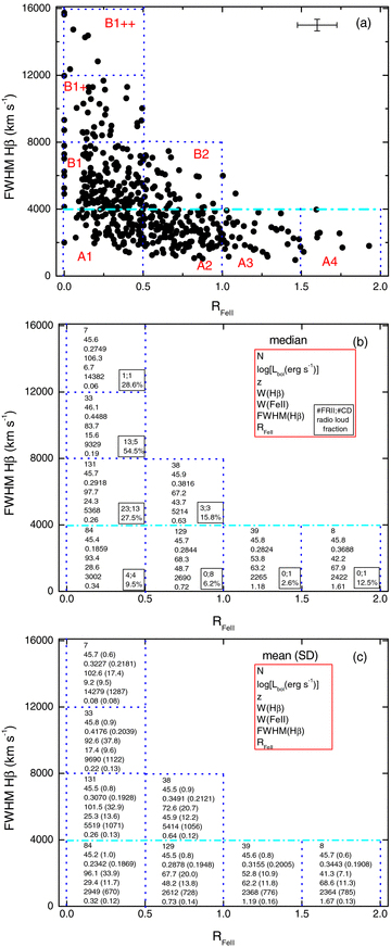
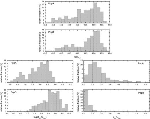
(a) The optical plane of the 4D Eigenvector 1 Parameter Space. The quadrants indicate the bins defined by Sulentic et al. (2002) and adopted here for composite spectra. Typical 2σ error bars are shown in the upper right corner. The horizontal dash–dot line indicates the nominal boundary between Populations A and B. The relative numerical contribution of from each population is 55 per cent in A and 45 per cent in B. (b) The number of sources considered in each bin along with a few (median) relevant measures in each bin are indicated. The square in the upper right is the legend of the numbers shown in each bin. Inside each bin (lower right square), we report the number of FR ii and core-dominated RL sources along with the estimated RL fraction. (c) Similar to (b), this time the numbers represent mean and standard deviations (in the parenthesis in each case).
NLSy1 sources, customarily defined by FWHM(Hβ) < 2000 km s−1, do not form a distinct class of objects relative to the bulk of Population A sources2 (Marziani et al. 2001) if we consider their optical/UV spectra (Véron-Cetty, Véron & Gonçalves 2001; Sulentic et al. 2002).
There is a remarkable change in the Hβ line profile at FWHM(Hβ) ≈ 4000 km s−1: Hβ is fit by a Lorentzian function up to FWHM(Hβ) ≈ 4000 km s−1, while a double Gaussian is needed for broader sources (Sulentic et al. 2002; Marziani et al. 2009).
It is interesting to note that if one uses the RQ–RL separation to define this boundary within the optical plane of the 4DE1 space (see table 3 and fig. 4 of Zamfir et al. 2008) then a 2D Kolmogorov–Smirnov (2D K–S) test yields FWHM(Hβ) ≈ 3900 km s−1. RQ–RL distinction appears less general and subordinated to the A/B framework since Population B sources can be both RQ and RL (Zamfir et al. 2008). We are not claiming that the limit at FWHM(Hβ) ≈ 4000 km s−1 is absolute or fixed. Several lines of evidence suggest a dichotomy at FWHM(Hβ) ≈ 4000 km s−1 (Sulentic et al. 2007; Marziani et al. 2009); especially impressive is the Hβ profile change mentioned above (and also discussed later in the paper), although as yet we cannot exclude the possibility that there is a smooth change of properties along the optical E1 sequence.
The first result listed above suggests that Population A sources are simply an empirically-motivated extension of the NLSy1s to a somewhat broader limit. The limit at FWHM(Hβ) ≈ 4000 km s−1 is also motivated by the rarity of sources with broader Hβ if RFe ii > 0.5. An underlying physical parameter could be the accretion rate, and the limit may be dependent on luminosity (see fig. 11 of Marziani et al. 2009 for the locus of fixed accretion rate in the FWHM versus luminosity plane). In this case, the effect of orientation may blur the boundary at a critical accretion rate potentially associated with a BLR structure transition, creating an almost constant limit at 4000 km s−1 at low and moderate luminosity. No break is observed near FWHM(Hβ) ≈ 4000 km s−1 in the 4DE1 optical plane, and it would be truly remarkable if one were present given also measurement uncertainties. Summing up, several lines of evidence from the previous work mandate the consideration of – at the very least – a limit at FWHM(Hβ) ≈ 4000 km s−1, lest gross errors and misconceptions are introduced in the data analysis.
The paper is organized as follows. Section 2 presents a detailed characterization of Hβ broad emission line in low-redshift SDSS spectra based on composite median spectra in two representative bins defined within the optical plane of the 4DE1 parameter space and a set of diagnostic measures like asymmetry, kurtosis and centroid shift. It also explores the connection between these diagnostic measures and the 4ED1 space. In Section 3, we compare sources of low and high Eddington ratio both in terms of line measures and composite median spectra. Sections 4 and 5 are dedicated to discussion and conclusions. Throughout this paper, we use Ho= 70 km s−1 Mpc−1, ΩM= 0.3 and ΩΛ= 0.7.
2 DETAILED CHARACTERIZATION OF Hβ EMISSION LINE PROFILES IN LOW-Z QUASARS
2.1 General remarks
The robustness of any systematic study of quasar broad emission lines is conditioned by two things: (a) availability of large, representative samples and (b) the quality of spectra, both in terms of resolution and S/N ratio. The situation is greatly improved thanks to dedicated surveys like the SDSS that make available to the community large, homogeneous data sets. This work involves exploitation of ∼470 bright low-z (<0.7) spectra from SDSS (DR5; Adelman-McCarthy et al. 2007). No comparable sample exists in terms of uniformity, completeness and spectroscopic quality. Construction and characteristics of the sample are explained in Zamfir et al. (2008). Our work focuses chiefly on the two optical dimensions of the 4DE1 space, with occasional commentaries relative to the other two based on previous studies. One goal of this study is to emphasize that composite average spectra – averaged in a well-defined context like 4DE1 space – can reveal the underlying stable components of the broad lines. We address or readdress a few fundamental questions in this paper.
Can we further emphasize quasar diversity employing measures such as centroid shifts, asymmetry and line kurtosis?
How are these diagnostics tied to and/or incorporated within the 4DE1 space (see also Boroson & Green 1992)?
Is the distinction between Population A/B more general than RL versus RQ quasars?
Does it reveal evidence for a Population A/B dichotomy or continuity across 4DE1?
Can we reveal/infer some kinematics/structural differences with the aid of the aforementioned line diagnostics?
The departure point for our present analysis is the sample of N= 477 bright SDSS (DR5) quasars (z < 0.7) defined in Zamfir et al. (2008). The sample was defined such that point spread function (psf) g or i-band magnitudes are brighter than 17.5, representative for the luminosity regime log [Lbol(erg s−1)]= 43–47. The redshift limit was chosen so that we have a good coverage of the Hβ and its adjacent spectral regions employed for the underlying continuum definition. The brightness limit on the apparent magnitude was driven by the need of good quality spectra, which allows reliable measures on the broad line profiles. Figs 1 and 2 present the general properties of the sample in terms of location in the optical plane of the 4DE1 space, other spectral properties of the broad lines, the number of FR ii and core-dominated RL sources along with the estimated RL fraction in each bin, and the S/N spectral quality, respectively. For a detailed presentation of the criteria involved in the construction of our sample please refer to section 2 of Zamfir et al. (2008).
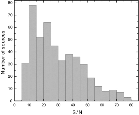
Distribution of the S/N measure (per pixel) in the 5600–5800 Å region for our sample of N= 469 sources.
Fig. 1(a) shows the source distribution in the optical plane of 4DE1 whose parameters involve broad Hβ, FWHM(Hβ), and the equivalent width ratio of the optical Fe ii (4570 Å blend) and broad Hβ, RFe ii≡ W(Fe ii4434−4684 Å)/W(Hβ). Sources show the characteristic ‘banana’ shape distribution found in earlier studies.
2.2 Spectral bins in the optical plane of the 4DE1
Bins of ΔFWHM(Hβ) = 4000 km s−1 and ΔRFe ii= 0.5 are shown in Fig. 1 following the definitions introduced in Sulentic et al. (2002). The width ΔRFe ii= 0.5 basically corresponds to the measurement uncertainty at ±2σ confidence level. For example, if we consider the centre of bin A2 (RFe ii= 0.75), data points are not significantly different from this central value at a confidence level ±2σ since the error of individual measurements is in the range ±0.20 to ±0.25. A few extreme sources with FWHM(Hβ) > 16 000 km s−1 or RFe ii > 2.0 are not considered here. The two sources that are located in what would be bin B3 are ignored at this time as well. The bulk of sources lie between FWHM(Hβ) = 1000–12000 km s−1 and RFe ii < 1.5. Our sample does not include a significant population of NLSy1 sources between FWHM(Hβ) = 500 and 1000 km s−1, which are classified as ‘Galaxy’ in the SDSS. Such SDSS sources have been tabulated by Zhou et al. (2006) and n= 40 of them were included for evaluation in Marziani et al. (2009). In our present report, we make use of the Fe ii optical template provided by Boroson & Green (1992) study, which is not suitable for very narrow broad lines. In only 14 sources (less than 3 per cent) do we measure a negligible RFe ii (see also Dong et al. 2009; Fe ii may be a ubiquitous signature in type 1 AGN and we speculate that Fe ii presence may be incorporated in the empirical definition of type 1 phenomenology). The median centroid of the source distribution is located at [RFe ii, FWHM(Hβ)]= (0.53, 4300 km s−1). The distribution shows no obvious concentration at the centroid values, instead we see a broader concentration between 0.1–1.0, 1000–6000 km s−1. The source distribution is ‘elongated’ (like a banana) and largely reflects the intrinsic source dispersion rather than measurements errors [∼20σ in FWHM(Hβ) and ∼16σ in RFe ii].
A trend is seen in the sense that narrower FWHM(Hβ) sources show a large dispersion in RFe ii and weaker RFe ii sources show a large dispersion in FWHM(Hβ). The range of RFe ii is similar at FWHM(Hβ) = 8000 or 12 000 km s−1 and the range of FWHM(Hβ) is the same at RFe ii= 1.0, 1.5 or 2.0. Sources with very broad FWHM(Hβ) and large RFe ii measures are not present in this sample of quasars and are likely either non-existent or obscured. The distribution shows tails at both sides, i.e. extreme FWHM(Hβ) (up to 40 000 km s−1, Wang et al. 2005) and extreme RFe ii (up to 2.5); the tails are mutually exclusive and they represent about 5 per cent of the total sample.
Figs 1(b) and (c) provide median and mean values for key parameters in each bin: the number of sources and average values of bolometric luminosity (Lbol≃ 10λLλ, where λ≡ 5400 Å, see Zamfir et al. 2008), redshift z, equivalent width of Hβ and of Fe ii (4570 Å blend), FWHM(Hβ) and RFe ii. These numbers are representative for quasars of intermediate (bolometric) luminosity (log Lbol[erg s−1]= 43.5–46.5) at low redshift (z < 0.7). RL sources tend to strongly prefer the Population B regime. None the less, there is a small fraction of RL amongst population A sources, but we should also emphasize that ∼40 per cent of them (7 out of 18) show FWHM(Hβ) in very close to the 4000 km s−1 A/B adopted boundary.
Comparing the average (median or mean) equivalent width values W(Hβ) and W(Fe ii)[Figs 1(b) and (c)], we see an increase of about 45 per cent in the former and a decrease of about 50 per cent in the latter measure in bin B1 relative to bin A2. RFe ii consequently decreases by a factor of 2.8 from A2 to B1. RL quasars strongly concentrate above FWHM(Hβ) ∼ 4000 km s−1 and below RFe ii∼ 0.50 (see fig. 4 of Zamfir et al. 2008). Most exceptions (i.e. Population A RL) show core dominated radio morphology suggesting that they are viewed near the radio jet axis. If Hβ emission arises from an accretion disc oriented perpendicular to the jets' axis then a correction to FWHM(Hβ) would move most core-dominated RL from Population A into the region of Population B (Marziani et al. 2003b). RL sources showing lobe-dominated FR ii and core-dominated radio morphologies show a clear and significant separation in the 4DE1 optical plane (Sulentic et al. 2003; Zamfir et al. 2008). This is a hint that the orientation plays an important role at least for RL quasars and possibly for all quasars.
A more extreme comparison [relative to Figs 1(b) and (c)] could involve the less populated bins A3, B2 and B1+, each with about 30–40 sources. Average luminosities are very similar. On average W(Fe ii) in bin A3 is about 4 times larger than in bin B1+. Average W(Hβ) in bin B1+ is about 1.5 times larger than in bin A3. There are no RL sources in bin A3, but a large concentration of RL is found in B1+ (see fig. 4 in Zamfir et al. 2008). We avoid bin A1 with the smallest FWHM(Hβ) and RFe ii measures because it may involve a mixture of Population A and B sources. In terms of spectral quality, we estimate mean and median ratio S/N ∼ 29 (defined in the continuum region 5600–5800 Å). Fig. 2 shows the (histogram) distribution of pixel S/N ratios for the N = 469 SDSS spectra in our sample.
2.3 Composite spectra of quasars
Composite average quasar spectra have proven to be a powerful tool for revealing both commonalities among and differences between quasars. High S/N spectral composites have served many purposes. First, they allowed a general description of the quasar phenomenon by (a) providing a reference or cross-correlation template spectrum by identifying (and measuring) weak emission features (strengths, widths, shifts, asymmetries, etc.), otherwise hardly observed in individual spectra (e.g. Wills et al. 1980; Véron-Cetty, Tarenghi & Véron 1983; Boyle 1990; Francis et al. 1991; Zheng et al. 1997; Vanden Berk et al. 2001; Constantin & Shields 2003; Scott et al. 2004; Glikman, Helfand & White 2006), (b) defining the underlying continuum by isolating wavelength regions (almost) free of lines (e.g. Francis et al. 1991; Vanden Berk et al. 2001; Constantin & Shields 2003), (c) revealing the omnipresence of Fe ii blends throughout the UV and optical domains (see e.g. section 4.2 in Vanden Berk et al. 2001 and references therein) and (d) evaluating colours of quasars and/or K(z) corrections (Cristiani & Vio 1990; Glikman et al. 2006).
As larger samples of quasars spectra became available, composites were constructed for sources with very similar properties like: (1) radio-loudness (e.g. Cristiani & Vio 1990; Zheng et al. 1997; Brotherton et al. 2001; Telfer et al. 2002; Bachev et al. 2004; Glikman et al. 2006; Metcalft & Magliocchetti 2006; de Vries, Becker & White 2006), (2) radio core-to-lobe flux density ratio (e.g. Baker & Hunstead 1995), (3) radio morphology, FR ii versus core-dominated, e.g. de Vries et al. (2006), (4) optical continuum slope or relative colour (Richards et al. 2003), (5) broad emission line velocity shifts (Richards et al. 2002; Hu et al. 2008b), (6) C ivλ1549 Å line width (Brotherton et al. 1994), (7) emission line widths and strengths (Sulentic et al. 2002; Constantin & Shields 2003; Bachev et al. 2004), (8) BH mass (MBH) and Eddington ratio (Lbol/LEdd) (e.g. Marziani et al. 2003b), (9) variability (Wilhite et al. 2005; Pereyra et al. 2006), (10) BAL (e.g. Brotherton et al. 2001; Richards et al. 2002; Reichard et al. 2003) and (11) soft X-ray brightness (e.g. Green 1998). Such composites facilitate an emphasis on differences between properties of quasars. The luminosity and redshift dependence/evolution of quasar properties was sought and tested with the aid of composite spectra (e.g. Cristiani & Vio 1990; Zheng et al. 1997; Blair et al. 2000; Croom et al. 2002; Corbett et al. 2003; Yip et al. 2004; Nagao et al. 2006; Scott et al. 2004; Bachev et al. 2004; Metcalft & Magliocchetti 2006; Marziani et al. 2009).
An important question involves how to combine individual spectra into a composite. Moreover, how well does a composite spectrum preserve the properties of the input components and to what extent is it representative of the sample from which it has been constructed? It has been noted that there is no unique best answer to such questions. While a median composite preserves the relative fluxes of the emission features, a geometric mean composite preserves better the shape of the underlying continuum (e.g. Vanden Berk et al. 2001). Additional questions can be related to how to weight each spectrum's contribution into the composite. Depending on the number and quality of individual spectra available one could decide whether a weighted-average (arithmetic mean) composite (e.g. Francis et al. 1991; Glikman et al. 2006) is more useful than a composite where all spectra are given equal weight (e.g. Constantin & Shields 2003). The most important thing is the context within which we define the composites; we consider 4DE1 is the best approach available.
Given the S/N distribution (Fig. 2) of our sample, the homogeneity of the SDSS spectra and the nature of our spectral analysis we see the median composites with equal weight from individual components as most suitable (for a discussion on the relevance of the median composites see section 4.1 of Bachev et al. 2004).
2.4 Hβ profile shape
2.4.1 Data analysis
Low-z rest-frame spectra require galaxy decontamination and flux corrections. They are normalized to the 5100-Å specific flux prior to being considered for the composite. The full analysis procedure for a quasar optical spectrum focusing on the Hβ region is outlined in Zamfir et al. (2008). We added an intermediate step in the present study by defining the underlying continuum as a simple power-law anchored in the regions 4195–4218 Å and 5600–5800 Å. The Fe ii template used to model Fe ii emission around Hβ is based on IZw1 (Boroson & Green 1992; Marziani et al. 2003a). The template matches the 4750 Å Fe ii‘blue’ blend significantly better than it does the Fe ii blend redward of [O iii]λ5008 Å (‘red’ blend). In many cases, the ‘red’ blend of Fe ii may be overestimated. In order to alleviate this problem, we opted for an additional iteration in the reduction process of the composite spectra: (1) we define the underlying power-law continuum, (2) subtract the continuum, (3) find the best match between the Fe ii template and the spectrum (adjusting the width and intensity of the template), focusing on the best match for the blue blend of Fe ii, (4) subtract this template solution from the original rest-frame spectrum (available before step 1) and (5) redefine a power-law continuum using the wavelength regions 4195–4218 and 5100–5300 Å. This continuum is slightly steeper than the initial choice. We now repeat steps 2 and 3. This iteration significantly improves the match between template and the red blend of Fe ii.
From the spectrum thus obtained (continuum and Fe ii-free), we cut out the wavelength range bracketed by He iiλ4687 Å and [O iii]λ5008 Å. We simultaneously fit all lines in the selected interval, allowing for narrow components (NC) in the case of He ii, Hβ, [O iii]λ4960 Å and 5008 Å lines. The [O iii] lines require an additional component, in most cases blueshifted relative to the quasar's rest frame indicated by the NC. We do not require a match in width between the NC of Hβ and the core (the narrower of the two) components of the [O iii] lines. We constrain the [O iii] 5008/4960 flux ratio R= 3 allowing for a maximum 15 per cent error. All components are modelled with Gaussian functions in the first stage. Subsequently, we test whether a Lorentzian function provides an improved fit to the Hβ broad component (BC) in terms of reduced χ2 and by visual inspection of residuals. All other emission lines are modelled with Gaussian functions. We use the Levenberg–Marquardt algorithm3 to adjust the parameter values in the iterative procedure.
2.4.2 Composite spectra in 4DE1
Figs 3 and 4 present composite spectra for bins A2 and B1, respectively. We show both the region (upper) from 3500 to 7000 Å with continuum+line model and an enlarged view (lower) of the Hβ region from 4600 to 5100 Å with details of the line model. We focus on bins A2 and B1 as a representative of source differences between Populations A and B. We avoid bin A1 because it likely contains a mix of both Population A and B as well as because it shows a range of RFe ii values that is too similar to bin B1 sources.
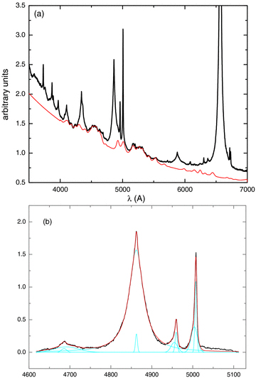
(a) Median composite spectrum of A2 bin sources and the best model of Fe ii emission around Hβ. (b) A simultaneous fit (our best solution) of Hβ and adjacent lines in the selected wavelength interval of the composite.

(a) Median composite spectrum of B1 bin sources and the best model of Fe ii emission around Hβ. (b) A simultaneous fit (our best solution) of Hβ and adjacent lines in the selected wavelength interval of the composite.
Extreme A bin composites (A3 and A4) tend to have stronger Fe ii emission while extreme B bins (B1+, B1++) involve sources with broader Hβ profiles and weaker Fe ii emission. The systematic weakening of Fe ii between bins B1 and B1++[see also Figs 1(b) and (c)] may be caused by the increase in FWHM for Fe ii lines that increases with FWHM(Hβ). As the Fe ii blends broaden they create a pseudo-continuum that may lead to systematic underestimation of Fe ii strength. However, thanks to the high S/N of our SDSS sample, Fe ii is detected for the first time in most sources with FWHM(Hβ) > 8000 km s−1, revealing that this effect is not as influential as feared.
Bins A2 and B1 are well matched in terms of number of sources as well as mean/median redshift and log Lbol[Figs 1(b) and (c)]. N= 129 and 131 sources were used to generate the A2 and B1 composites, respectively. The differences between the two composites would be slightly larger if we included in A2 the NLSy1s sources with FWHM(Hβ) < 1000 km s−1 tabulated by Zhou et al. (2006). However, inclusion or exclusion of these sources will make no significant change in the results. Marziani et al. (2003b) show that sources with FWHM(Hβ) < 2000 km s−1, often described as a separate class, are similar in terms of line profile shape (i.e. Lorentzian) to those having FWHM(Hβ) in the range 2000–4000 km s−1.
The A2 median composite shows high enough S/N to reveal a modest inflection between the BC and NC of Hβ. The NC adopted by the model shows FWHM ∼ 350 km s−1, very similar to the core components of the [O iii] lines. BC shows FWHM(Hβ) ≃ 2600 km s−1. The best fit [Fig. 3(b)] to the BC of Hβ profile is obtained with a Lorentzian function, confirming results of previous studies (Sulentic et al. 2002; Marziani et al. 2003b, 2009). The profiles of NLSy1 sources have long been described as Lorentzian (Véron-Cetty et al. 2001), but that profile description now extends to FWHM(Hβ) ≈ 4000 km s−1. A Gaussian fit does not provide satisfactory results in light of χ2 residuals. A pair of unshifted Gaussians provides a reasonable fit (Popović et al. 2004; Bon et al. 2009) since they essentially represent an approximation of a Lorentzian. A Lorentzian is preferred as a description of the A2 Hβ profile based on χ2. The broad Lorentzian component shows no shift relative to the quasar's rest frame.
There is a positive residual redward of [O iii]λ5008 Å. This residual can be an artefact produced by a mismatch between the Fe ii template and the composite spectrum coupled with an oversimplified definition of the underlying continuum. The red shelf has been pointed out in Marziani et al. (2003a) (see their section 4.3) and Véron, Gonçalves & Véron-Cetty (2002). The latter study focused on two sources with such a prominent feature and showed that the main contributors to the ‘shelf’ are most probably the He i lines λλ 4922, 5017 Å and is not caused by a broad redshifted component of Hβ or [O iii] lines. Even if a very broad line region (VBLR) is assumed in our case here and affects or causes the red ‘shelf’, its contribution to the total flux of Hβ is no more than 10 per cent, which is within the uncertainty range of the fitting routine.
The median composite for bin B1 (Fig. 4) shows striking differences from the A2 composite, most notably in the shape of the broad Hβ profile. We see two inflections: (1) between the NC and the BC and (2) on the red side of the BC. The simplest fit to the BC therefore requires a double Gaussian involving a broad (BC) unshifted and a very broad component (VBC), redshifted by ∼1500 km s−1, which also involves about 53 per cent of the total Hβ broad line flux. This model is again in agreement with our earlier studies. Detection and measurement of the VBC requires spectra with good S/N and moderate resolution – the median composite suggests that it is very common if not ubiquitous in sources with FWHM(Hβ) > 4000 km s−1. It is obvious that some or many sources show FWHM(Hβ) > 4000 km s−1 because of this second component. If we interpret the unshifted BC as the classical BLR then we might expect it to show a Lorentzian shape. Fitting the B1 composite with an unshifted Lorentzian plus redshifted Gaussian yields a poorer χ2 and a VBC comprising less than ∼10 per cent of the total broad line flux, with ∼6000 km s−1 redshift. Past and present results suggest that a double Gaussian is the best choice. The classical ‘unshifted’ BC Gaussian shows a only small blueshift of ∼−100 km s −1 and FWHM of ∼4000 km s−1.
The width of the BC component in the bin B1 composite is significantly less than the median value of FWHM(Hβ) ∼ 5400 km s−1 reported for bin B1 in Fig. 1(b). We conclude that FWHM measures of broad Hβ that do not correct for the VBC will lead to serious BH mass overestimates. At the same time, for the bin A2 there is no difference between the median value reported in Fig. 1(b) and the measured FWHM(Hβ) in the composite median spectrum. This suggests that no VBC correction is required for Population A sources making their Hβ-based BH mass estimates more reliable. The bin A2–B1 comparison suggests fundamental structural and kinematic differences between Population A and B sources (see also Sulentic et al. 2002) most likely coupled with non-trivial effects of orientation.
2.4.3 Diversity of Hβ profiles of individual spectra
We have argued that indiscriminate averaging of spectra will obscure the most physically fundamental differences in a source sample. The purpose of this section is to go to the other extreme and examine source spectra individually. Fig. 5 shows a selection of individual Hβ profiles in order to illustrate that all previously known (e.g. Stirpe 1990) diversity is present in the SDSS sample. The A2 and B1 median composite spectra presented and discussed earlier (and also discussed in Sulentic et al. 2002) do not show the variety of features observed in individual, single-epoch spectra shown in Fig. 5. This justifies the interpretation that average spectra represent the underlying commonality, more stable components in the Hβ profiles of different sources. The individual spectra are, to some extent, equivalent to the results of spectroscopic monitoring of a single source. Since many of the features do not show up in the composite they presumably represent relatively short-lived, transient and therefore lees important changes in the profiles.
![A selection of Hβ profiles meant to illustrate the diversity of asymmetries, shapes and shifts in individual sources. A magenta dash–dot vertical line in each case indicates the rest frame defined by Hβ NC at λ4862.7 Å (Note that we refer our measures to vacuum rest-frame wavelength values). A blue dotted vertical line indicates the peak of the broad Hβ defined at 9/10 fractional intensity. In a few panels, a third vertical line indicates the rest-frame [O iii]λ5008.2 Å and the actual blueshifted position of that line. The displayed spectra still include the Fe ii contribution, but the Hβ measures employed in the paper are performed on Fe ii-‘cleaned’ profiles. Panels are grouped by bins and displayed in order of increasing asymmetry index A.I.(1/4) within each bin. In each case, we also provide a set of numbers: bin, bolometric luminosity, S/N measures in the continuum (see Fig. 2), asymmetry and kurtosis indices, centroid shift at 1/4 and 9/10 fractional intensity.](https://oup.silverchair-cdn.com/oup/backfile/Content_public/Journal/mnras/403/4/10.1111_j.1365-2966.2009.16236.x/1/m_mnras0403-1759-f5a.gif?Expires=1750251561&Signature=iALor2xwzslVNoTjXkbPfnrMyKQSD7vJ5e5Zik8CuAThjip5ox6KieU1fPxm924e0ystI0IiiNA6qCzsnxjrhAZC9-GtwdC1FHqsCUTbHaZg9E0LJJM1MLojhHj0u7BOc6j5k5v4YUZKh4nhR5DqnYsPULdAhHsW6rrKSZm4znmJSl5-E7sRTlDWwF2pGeMLtyvy-zXAdDPXbtaPtgFxd21NxkpQN~hZayOIvXJ6a0IW293pGPec87kRLMBTYKLT-6-rJB8wtx173HlY9eKOVKnfRwZEd3BYEogNOS06zn9zv~5yrL8wUG8HayxvmKT5ZYnSrZUadcv8Nz4rjtxsQw__&Key-Pair-Id=APKAIE5G5CRDK6RD3PGA)
![A selection of Hβ profiles meant to illustrate the diversity of asymmetries, shapes and shifts in individual sources. A magenta dash–dot vertical line in each case indicates the rest frame defined by Hβ NC at λ4862.7 Å (Note that we refer our measures to vacuum rest-frame wavelength values). A blue dotted vertical line indicates the peak of the broad Hβ defined at 9/10 fractional intensity. In a few panels, a third vertical line indicates the rest-frame [O iii]λ5008.2 Å and the actual blueshifted position of that line. The displayed spectra still include the Fe ii contribution, but the Hβ measures employed in the paper are performed on Fe ii-‘cleaned’ profiles. Panels are grouped by bins and displayed in order of increasing asymmetry index A.I.(1/4) within each bin. In each case, we also provide a set of numbers: bin, bolometric luminosity, S/N measures in the continuum (see Fig. 2), asymmetry and kurtosis indices, centroid shift at 1/4 and 9/10 fractional intensity.](https://oup.silverchair-cdn.com/oup/backfile/Content_public/Journal/mnras/403/4/10.1111_j.1365-2966.2009.16236.x/1/m_mnras0403-1759-f5b.gif?Expires=1750251561&Signature=T5F7mcdIWk-lsDmTyWISTydlnHxa0SLc0v725TvEQSd0fRLH2sQcnoVDFUZIbs5e7pZatFNy0RbEh0466WjkgvVmDGRjbPfdSxzFle8Fbz3jSuNvCmUnHBmv0iyxTlfBiIIQOqoLw1u0IwOtcpTWlbdyS7YtucnaPPhR-A-CGwg2gkhXwrUPI8K45OcqVMw~UxRfD0ery0JGC~iTFbirLMHDkp-qswvsJXwbhAp8nkH321FeT0xpVX0TT4At9cwhvuhSwLLnDRRMA4fHNK7uge3JeMDx6dr5QQ-oqjVaNzKhJ7qOFSLVMYTL-k4St4Vtomh1-Tmz94V-aLnmd3~j9Q__&Key-Pair-Id=APKAIE5G5CRDK6RD3PGA)
![A selection of Hβ profiles meant to illustrate the diversity of asymmetries, shapes and shifts in individual sources. A magenta dash–dot vertical line in each case indicates the rest frame defined by Hβ NC at λ4862.7 Å (Note that we refer our measures to vacuum rest-frame wavelength values). A blue dotted vertical line indicates the peak of the broad Hβ defined at 9/10 fractional intensity. In a few panels, a third vertical line indicates the rest-frame [O iii]λ5008.2 Å and the actual blueshifted position of that line. The displayed spectra still include the Fe ii contribution, but the Hβ measures employed in the paper are performed on Fe ii-‘cleaned’ profiles. Panels are grouped by bins and displayed in order of increasing asymmetry index A.I.(1/4) within each bin. In each case, we also provide a set of numbers: bin, bolometric luminosity, S/N measures in the continuum (see Fig. 2), asymmetry and kurtosis indices, centroid shift at 1/4 and 9/10 fractional intensity.](https://oup.silverchair-cdn.com/oup/backfile/Content_public/Journal/mnras/403/4/10.1111_j.1365-2966.2009.16236.x/1/m_mnras0403-1759-f5c.gif?Expires=1750251561&Signature=QxCs4-SC6vtaA~E11nCx-UpCNnXeJlL7unum8l6kKNjCac2LaTPcXBZIC~03cS890NvbuNZyTWBuq9cuVlWJUvjx9sNxRdfHvwssKcHc4r8v3S53Fd2D~4789rHboV~8uhowliJ2Oq-aPdtJEpPCKwEc13fCU-wg1Ak~W9uymr4u7AkYtoGlo0trt3YDnUFhp0mLaTW7guTYo-b5E-ftWgI~u~IIUNCspTQX~6pOXTbCNloOVqzLLnqsFamHLU3tvcVMbZBDMX6jcLV-2MsJwbsGu9kf5JTErqCckGQ02K4RdgBXygeoZO8ibprX1TuQQd86gLCy~-PRmhdA8F21Wg__&Key-Pair-Id=APKAIE5G5CRDK6RD3PGA)
![A selection of Hβ profiles meant to illustrate the diversity of asymmetries, shapes and shifts in individual sources. A magenta dash–dot vertical line in each case indicates the rest frame defined by Hβ NC at λ4862.7 Å (Note that we refer our measures to vacuum rest-frame wavelength values). A blue dotted vertical line indicates the peak of the broad Hβ defined at 9/10 fractional intensity. In a few panels, a third vertical line indicates the rest-frame [O iii]λ5008.2 Å and the actual blueshifted position of that line. The displayed spectra still include the Fe ii contribution, but the Hβ measures employed in the paper are performed on Fe ii-‘cleaned’ profiles. Panels are grouped by bins and displayed in order of increasing asymmetry index A.I.(1/4) within each bin. In each case, we also provide a set of numbers: bin, bolometric luminosity, S/N measures in the continuum (see Fig. 2), asymmetry and kurtosis indices, centroid shift at 1/4 and 9/10 fractional intensity.](https://oup.silverchair-cdn.com/oup/backfile/Content_public/Journal/mnras/403/4/10.1111_j.1365-2966.2009.16236.x/1/m_mnras0403-1759-f5d.jpeg?Expires=1750251561&Signature=zVCSXs1PQJlsrq3NhiLl2ytd0z45rEJZWzY-2khulxpjNxRStwkNzeGkIBaTLZauu0USrqm25BtYt7qkwGqauALgN-VE7aEwnofnAlRjbDio08wEYSz1cxFXOpKSKONBM4eUp1ErqfpcfpzKdmMhFym0X8zKV7~6GM9ui5ZTN1x2IHN8XY~bvw2oC6VgYWcrG6el00aiMulGUlmKbR2ybnbj57hvej3pFbiHrSAhCNInyAuBq2sERC4EHt2SFo5H5ShHR4LXpT7eNzVdTTSWfWgH5IujXsGIADsW4zKZRfZEmkNoRfrWZoIBiEO3wzwjLEG-hDrdZ3XfQhRy8D2tPg__&Key-Pair-Id=APKAIE5G5CRDK6RD3PGA)
A selection of Hβ profiles meant to illustrate the diversity of asymmetries, shapes and shifts in individual sources. A magenta dash–dot vertical line in each case indicates the rest frame defined by Hβ NC at λ4862.7 Å (Note that we refer our measures to vacuum rest-frame wavelength values). A blue dotted vertical line indicates the peak of the broad Hβ defined at 9/10 fractional intensity. In a few panels, a third vertical line indicates the rest-frame [O iii]λ5008.2 Å and the actual blueshifted position of that line. The displayed spectra still include the Fe ii contribution, but the Hβ measures employed in the paper are performed on Fe ii-‘cleaned’ profiles. Panels are grouped by bins and displayed in order of increasing asymmetry index A.I.(1/4) within each bin. In each case, we also provide a set of numbers: bin, bolometric luminosity, S/N measures in the continuum (see Fig. 2), asymmetry and kurtosis indices, centroid shift at 1/4 and 9/10 fractional intensity.
We want to go beyond the optical plane of the 4DE1 space because we find that sources inside bins like A2 and B1, while showing similar FWHM(Hβ) and RFe ii, also show considerable profile diversity implying that the two measures, width and relative strength of Fe ii emission, are not enough to characterize the diversity. For each spectrum shown in Fig. 5, we also indicate the bin in the optical plane of the 4DE1 space, the bolometric luminosity, spectral continuum S/N (as defined earlier) along with measures of centroid shifts, asymmetry and line shape (see next section). This set of 32 spectra is assumed representative in terms of S/N ratio, luminosity and occupation of the 4DE1 optical plane. In addition to the already stated purpose of presenting the great variance of the Balmer Hβ line properties amongst our low z/intermediate luminosity sample, this subset serves also the purpose of estimating typical uncertainties for the line diagnostic measures described in detail in the next section.
2.4.4 Higher order moments of Hβ profiles as diagnostics of the BLR Physics
In order to get a deeper insight into the hypothesized existence of two quasar Populations A and B (e.g. Sulentic et al. 2007; Marziani et al. 2009), we examine the sample distributions of higher order moments of the Hβ profiles. We focus on centroid shifts, asymmetry and kurtosis (line shape). The Hβ profile is fit with a high-order polynomial making no assumptions about different components that might be present. Higher order moments of the broad lines are affected by larger uncertainties than the linewidth measures, none the less, they offer the possibility to further constrain physical models of the BLR. We benefit in this analysis from the uniformity of SDSS spectra in S/N and resolution.
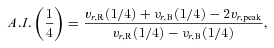
The vr,R and vr,B refer to the velocity shift on the red and blue wing, respectively (at the specified height of the profile), calculated relative to the rest-frame of the quasar. By ‘peak’ we mean 9/10 fractional intensity. The centroid shift will refer to x= 1/4 fractional intensity (what we call the line ‘base’) or x= 9/10 (the line ‘peak’). We point out that all these measures avoid the region below 1/4 fractional intensity due to the larger uncertainties associated with the definition of line wings and underlying continuum plus Fe ii pseudo-continuum.
2.4.5 Higher order moments and the optical plane of the 4DE1 parameter space
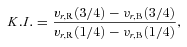
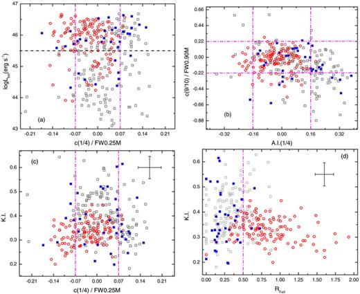
It is important to identify any kind of relation between 4DE1 and higher order diagnostic parameters that characterize the profile of the Hβ profile. Fig. 6 shows plots of FWHM(Hβ) versus the newly defined diagnostic measures: (a) versus asymmetry index A.I.(1/4), (b) versus kurtosis line shape measure K.I., (c) versus normalized base shift c(1/4)/FW025M and (d) versus normalized peak shift c(9/10)/FW0.90M). Whenever shown, the two vertical lines indicate the 2σ uncertainty lever on either side of zero. We also indicate the two Populations A and B defined in terms of FWHM(Hβ) less than and larger than 4000 km s−1, respectively. In each panel, we also display the FR ii radio sources with distinct symbols (blue solid). A few commentaries may be worthwhile. (1) There seems to be a trend in panel (a) in the sense that lower widths profiles are more symmetric, but sources with broader profiles show a numerical excess of (larger than the 2σ uncertainty) of red-asymmetric basis; (2) panel (b) shows no clear trend, but it indicates that the kurtosis values of broader Hβ profiles cover more uniformly a wider range of vales than the narrower profiles; (3) panel (c) reveals bears some similarity to panel (a), with a subtle difference; at lower widths there seems to be a slight excess of blueshifted ‘basis’, and the slight excess of redshifted basis is still apparent for broader profiles; (4) there is clear excess of sources with blueshifted ‘peaks’ over the whole range of FWHM. FR ii sources do not seem to have any special behaviour when contrasted against the other Population B sources.
Plots of FWHM(Hβ) versus (a) line asymmetry, (b) shape measure kurtosis, (c) ‘base’ normalized shift c(1/4)/FW0.25M and (d) ‘peak’ normalized shift c(9/10)/FW0.90M. The vertical lines indicate the 2σ uncertainty on either side of zero in all but panel (b). In the case, we also show the median typical 2σ error bars. The horizontal line at 4000 km s−1 is the Population A/B boundary proposed in the context of the 4DE1 space. The FR ii sources are shown with distinct blue symbols in each case.
The centroid shift measures are normalized in each case to the width of the profile at that same fractional intensity. We distinguish in each case Population A and B sources, as defined in the context of the 4DE1 parameter space. The vertical dotted lines indicate the 2σ median uncertainty derived for the subset of 32 sources shown in Fig. 5. Individual source profile uncertainties (for the 32 spectra) are estimated allowing for ±5 per cent variation in fractional intensity and then propagating the errors into the final diagnostic measure. Thus, the typical errors are: 2σ[A.I.(1/4)]≃ 0.16, 2σ[c(1/4)/FW0.25M(Hβ)]≃ 0.07, 2σ(K.I.) ≃ 0.092, 2σ[c(9/10)/FW0.90M(Hβ)]≃ 0.22, 2σ[c(1/4)]≃ 520 km s−1 and 2σ[c(9/10)]≃ 320 km s−1.
Figs 7(a)–(d) show the histogram distributions of the asymmetry index A.I.(1/4), the centroid shift at 1/4 and 9/10 fractional intensities c(1/4) and c(9/10), respectively, and the kurtosis measure K.I. The width of the bins in Figs 7 and 8 are chosen such that they are approximately equal to 1σ typical (i.e. average) uncertainty. In Table 1, we present the average (mean and median) values of the parameters shown in Fig. 7. We make the following comments relative to Fig. 7: (i) Population B sources show an excess (outside 2σ) of red asymmetric profiles and profiles red-shifted at the base, (ii) Population A sources are more symmetric and they show a slight excess of blue-shifted profiles at 1/4 from zero-level, (iii) there is an excess of blue-shifted peaks in both Population A and B sources and (iv) Population B sources show an extended tail of large kurtosis values, while Population A quasars show a more symmetric distribution about K.I. = 0.35, with a clear preference for lower K.I. values. A 1D K–S test indicates a 4 per cent probability of null hypothesis when comparing the normalized ‘peak’ shift distributions (lower left panel of Fig. 7). For all other measures shown in Fig. 7, a 1D K–S test shows a null-hypothesis probability less than 10−4. The numbers in Table 1 appear to confirm the aforementioned observations (i) and (ii).
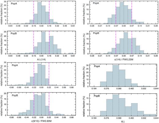
Histogram distributions of the asymmetry index A.I.(1/4) – upper left, base centroid shift c(1/4) normalized to FW0.25M – upper right, peak centroid shift c(9/10) normalized to FW0.90M – lower left and line shape kurtosis index K.I. – lower right. We show separately the distributions for Population A and B sources for each measure. The width of the bins is equal to σ estimated typical error. The vertical lines indicate a ±2σ interval on either side of 0 for the first three parameters.
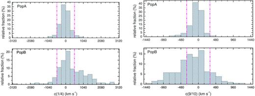
Histogram distributions for the centroid shifts at the base (1/4 fractional intensity) and peak (9/10 fractional intensity) without normalization to the width of the profile. Population A and B are illustrated separately. The width of the bins is equal to σ estimated typical error. The vertical lines indicate a ±2σ interval on either side of 0 in each case.
Average values for line asymmetry, kurtosis, base and peak shift for the two Populations A and B, relative to Fig. 7.
| Parameter | Population A (N= 260) Mean (SD); Median | Population B (N= 209) Mean (SD); Median |
|---|---|---|
| A.I.(1/4) | 0.002 (0.118); 0.001 | 0.096 (0.155); 0.083 |
| K.I. | 0.356 (0.063); 0.350 | 0.383 (0.092); 0.374 |
| c(1/4)/FW0.25M | −0.011 (0.062); −0.010 | 0.029 (0.076); 0.024 |
| c(9/10)/FW0.90M | −0.064 (0.277); −0.042 | −0.102 (0.300); −0.080 |
Fig. 8 shows a comparison of ‘base’ and ‘peak’ shift for Populations A and B, this time without normalization to the linewidth at the corresponding fractional intensity as in Fig. 7. We are aware that the un-normalized centroid shift values are less meaningful than the normalized ones. None the less, the two panels in Fig. 8 seem to show: (1) the two populations are significantly different (Population A sources being distributed mostly within ±2σ, while Population B quasars showing large excesses of blueshifted peaks and redshifted basis outside the 2σ range and (2) the measured shifts are quite large, ‘base’ redshifts over 1500–2000 km s−1 and ‘peak’ blueshifts in excess of −1000 km s−1 being observed.
We tested whether the observed distributions are spurious effects of the S/N. For this task, we reconstructed the histogram distributions shown in Fig. 7 restricting the sample to sources of S/N < 15 (∼20 per cent of our whole sample; see Fig. 2). All distributions presented above are confirmed and are not caused by the spectral S/N. We also tested if the distributions presented in Fig. 7 are driven by the preferential addition of a subset of SDSS quasars selected with some restriction on their radio properties (Zamfir et al. 2008). For this reason, we isolated only the RQ sources of our sample (i.e. N= 388 sources with log L21 cm < 31.6 erg s−1 Hz−1). Although we do not show the new histograms here, the distributions are qualitatively very similar to those in Fig. 7, thus we have clear indication that the population A/B concept is more general than the RL/RQ distinction.
The pioneering study of Boroson & Green (1992) incorporated measures of asymmetry, line shape and shift in their set of quasar spectral measures. They reported a significant correlation between RFe ii and the asymmetry of Hβ (see their fig. 5). Sources with strong Fe ii emission tend to show a flux excess on the blue wing of Hβ and the weaker Fe ii emitters tend to be shown more red-asymmetric Hβ profiles. The larger sample under investigation here reenforces their result [Figs 9(a) and (b)], the trend being clearly illustrated in diagrams that combine A.I.(1/4), c(1/4)/FW0.25M and RFe ii.
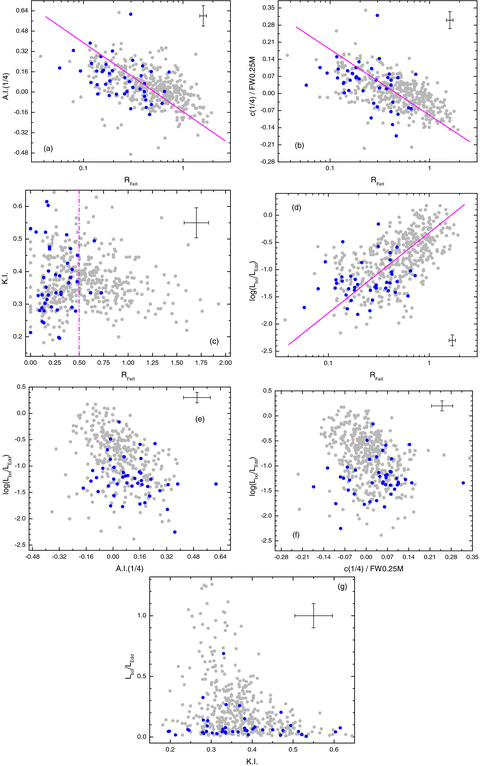
The connection between the line diagnostic measures and the Eigenvector 1 optical parameters and its chief driver, Eddington ratio. Darker symbols indicate (in each panel) the FR ii sources of our sample, assumed to be the parent population of RL quasars along with typical 2σ error bars in the corner of the panel. (a) The asymmetry index is plotted as a function of RFe ii. The bisector fit is also indicated. (b) The normalized base centroid shift is plotted as a function of RFe ii and the bisector fit is also shown. (c) The line shape measure kurtosis index K.I. is plotted as against RFe ii. The vertical line suggests a possible separation of two different trends around 0.50 abscissa value. (d) Eddington ratio is shown as a function of RFe ii along with a bisector fit. Panels (e) and (f) show the relation between base measures A.I.(1/4) and normalized centroid shift c(1/4)/FW0.25M and the Eddington ratio, the main driver of the 4DE1 diversity. Panel (g) shows the plot of Lbol/LEdd versus K.I.
Fig. 9 presents the most interesting plots involving pairs of measures from the following set: RFe ii, A.I.(1/4), c(1/4)/FW0.25M, K.I., Lbol/LEdd. The plots involving the peak shift are not shown because they do not illustrate any particularly special aspects beyond the already mentioned ones (related to the histograms in Fig. 7).
Figs 9(a) and (b) (log-linear plots) show the correlations between 4DE1 parameter RFe ii and the asymmetry and ‘base’ line shift measures. We also identify sources showing FR ii radio morphology symbols (dark blue). The FR ii quasars also serve as an independently (radio) defined subsample of Population B sources. Both panels show a trend from blue asymmetries/shifts at large RFe ii values to red asymmetries/shifts at lower RFe ii values. A Pearson correlation test applied shows to the whole sample yields a coefficient of rp=−0.50 (with a probability of not being correlated P∼ 0) for panel (a) and rp=−0.58 (P∼ 0) for panel (b). The bisector fit (Isobe et al. 1990) for (a) corresponds to the linear relation A.I.(1/4) =−0.54 log RFe ii− 0.15 and for (b) c(1/4)/FW0.25M =−0.27 log RFe ii− 0.09.
It is interesting to point out that in both cases the linear regression indicates that when the c(1/4) or A.I.(1/4) yield a null value, the corresponding RFe ii∼ 0.5. The majority of FR ii sources lie below the bisector fits and show positive A.I.(1/4) and c(1/4) values. This indicates that Population A sources are less asymmetric and less redshifted (at profile ‘base’) than Population B quasars (see also Fig. 19 and related discussion). A 2D K–S test for RL versus non-RL quasars within the optical plane of the 4DE1 space (Zamfir et al. 2008) indicates the same RFe ii∼ 0.50 as a relevant boundary.
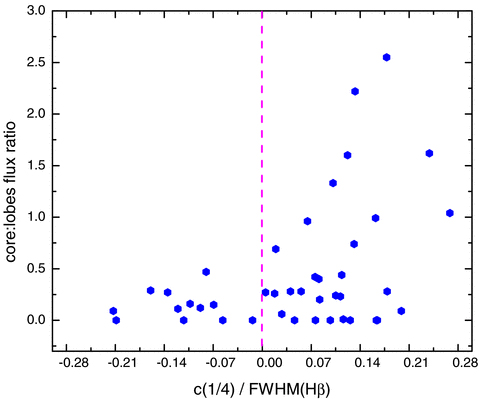
The FR ii sample is shown here in terms of core:lobes flux density ratio at 1.4 GHz, based on FIRST and the normalized Hβ emission line base shift. The vertical line indicates an unshifted measure.
Fig. 9(c) shows the plot of RFe ii versus the line shape K.I. measure. We see a complex distribution, quite different from Figs 9(a) and (b). We see different trends on either side of RFe ii∼ 0.5.
The parent population of RL quasars (FR ii sources) seems to prefer almost exclusively the region to the left of RFe ii= 0.50. Thus, we may already have several lines of evidence that seem to suggest RFe ii= 0.50 as a viable alternative to the original FWHM(Hβ) = 4000 km s−1 Population A–B boundary.
A Pearson test yields rp= 0.56 (P∼ 0) and a Spearman correlation test yields rs= 0.59 (P∼ 0). We show the bisector fit (correlation coefficient ρ= 0.58). The linear fit log(Lbol/LEdd) = 1.47 log RFe ii− 0.32 indicates that RFe ii= 0.50 corresponds to an Eddington ratio Lbol/LEdd= 0.18. Fe ii emission increases in strength relative to Hβ as the Eddington ratio increases, i.e. higher accretion rate. We are now in a position to test whether the base asymmetry and centroid shift measures A.I.(1/4) and c(1/4)/FW0.25M are correlated with the accretion rate measured by Lbol/LEdd. Figs 9(e)–(f) show the two line diagnostic measures versus log(Lbol/LEdd). For the plot involving the A.I.(1/4) (panel e), a Pearson test gives rp=−0.39 and a Spearman test gives rs=−0.43 (P∼ 0 in each test). For panel (f) rp=−0.28(P∼ 7 × 10⁻¹⁰) and rs=−0.32 (P∼ 6 × 10⁻¹³). The FR ii sources prefer the low-accretion regime. It appears that both the A.I. and the normalized c(1/4) measures are intimately connected to the 4DE1 parameter space. None the less, their inclusion in this space definition may not necessarily lead to an extension of the number of dimensions. One of the two indices may be regarded as a meaningful surrogate for FWHM parameter for example, although the problem requires further investigation.
Fig. 9(g) shows the plot of the Eddington ratio versus the line shape measure K.I.; the large majority of FR ii sources are low-accreting sources and their kurtosis measures spread over a wide range of values. It also seems to indicate that high Eddington ratios and large kurtosis values are mutually exclusive.
3 LOW VERSUS HIGH Lbol/LEdd SOURCES
Several recent articles (Hubeny et al. 2000; Marziani et al. 2003b; Collin et al. 2006; Bonning et al. 2007; Hu et al. 2008a; Kelly et al. 2008; Marconi et al. 2009) came from various directions to the conclusion that around some critical Lbol/LEdd∼ 0.2 ± 0.1 the properties/structure of the active nucleus may change fundamentally, thus providing support for the notion that two distinct populations of quasars exist (Collin et al. 2006; Sulentic et al. 2007). While the concept of two Populations A and B is deeply anchored into a long series of empirical studies (see section 3 and table 5 of Sulentic et al. 2007 for a summary), the nominal boundary at 4000 km s−1 FWHM(Hβ) may not have a very intuitive or immediate physical meaning or may even appear arbitrary. However, it is solely intended as a critical empirical measure that could indicate a fundamental change in the structure, geometry and kinematics of the BLR.
It has been suggested (as was emphasized earlier) that the Eddington ratio Lbol/LEdd is the main physical driver of the Eigenvector 1 parameter space variance. Our sample reenforces these arguments [e.g. Fig. 9(d)]. Fig. 10 compares the histogram distributions of bolometric luminosity Lbol, BH mass MBH and Eddington ratio Lbol/LEdd for populations A and B. Taken at face value they suggest that the two populations have very different distributions of MBH and Eddington ratio, even though they show similar luminosity distributions (see Table 2). Obviously, given that the two populations have similar luminosity distributions, the statistical difference in BH mass and Eddington ratio is a natural and direct consequence of the linewidth alone. Populations A and B being defined based on the FWHM(Hβ). A 1D K–S test in each case indicates a 1.2 per cent null-hypothesis probability for the bolometric luminosity distribution of the two populations and a probability less than 10−4 for the other two parameters. However, although the AGN central mass and the Eddington ratio may be more physically meaningful quantities, FWHM is a more direct and robust measure, much less affected by uncertainties and derived with fewer assumptions.
Population A and B quasars show similar luminosity distributions, but strikingly different distributions in terms of BH mass and Eddington ratios, Population A typically showing smaller BH masses and higher accretion rates and population B harbouring more massive BH and accreting much slower.
Average values for bolometric luminosity, BH mass and Eddington ratio for the two Populations A and B, relative to Fig. 10.
| Parameter | Population A (N= 260) Mean (SD); Median | Population B (N= 209) Mean (SD); Median |
|---|---|---|
| log[Lbol(erg s−1)] | 45.4 (0.9); 45.6 | 45.6 (0.8); 45.8 |
| log[MBH(M⊙)] | 7.8 (0.7); 7.9 | 8.7 (0.6); 8.8 |
| Lbol/LEdd | 0.36 (0.28); 0.28 | 0.07 (0.05); 0.06 |
| Parameter | Population A (N= 260) Mean (SD); Median | Population B (N= 209) Mean (SD); Median |
|---|---|---|
| log[Lbol(erg s−1)] | 45.4 (0.9); 45.6 | 45.6 (0.8); 45.8 |
| log[MBH(M⊙)] | 7.8 (0.7); 7.9 | 8.7 (0.6); 8.8 |
| Lbol/LEdd | 0.36 (0.28); 0.28 | 0.07 (0.05); 0.06 |
We decided to construct two test samples which would be representative of high and low accretors; all sources with Lbol/LEdd > 0.3 (N= 123) and with Lbol/LEdd < 0.1 (N= 177) are assumed to be high- and low-accretion quasars, respectively. This distinction turns out to be representative of the previously adopted populations A and B. All high Lbol/LEdd in our definition are part of population A and 87 per cent of the low Lbol/LEdd are population B, only 13 per cent spilling over the 4000 km s−1 boundary into population A. Obviously, we are aware that this kind of distinction would automatically introduce some bias, i.e. the low accretors would prefer larger BH masses and less luminous sources, and the high accretors would populate more the high luminosity and low BH mass regime.
We point out a few remarkable results in Figs 11(a)–(d). Panel (a) shows source luminosity as a function of the normalized centroid shift at line ‘base’ (1/4 fractional intensity). The bias indicated previously is clearly apparent. We may however focus on the region log Lbol[erg s −1] > 45.5, where both high- and low-accretor sources are well represented. There is a clear separation of the two samples in terms of base shift, with high accretors showing a preference for blueshifts and the low accretors for redshifts. Inside the ±2σ uncertainty interval, there is some overlap while outside (most significant ‘base’ line shifts) the separation is almost total. A few FR ii sources show blueshifted profiles at 1/4 base and very few high accretors spill over the +0.07 boundary into the redshifted region.
Two subsamples of N= 177 low (Lbol/LEdd < 0.1) and N= 123 highly accreting (Lbol/LEdd > 0.3) sources are considered, the squares representing the former and the circles showing the latter. The filled symbols indicate the FR ii sources. Pairs of vertical and horizontal lines on either side of zero show the typical ±2σ median uncertainty. (a) The bolometric luminosity versus the base (1/4 fractional intensity) normalized shift. The horizontal line at 45.5 ordinate indicates the values above which both samples are well represented numerically (see text). (b) The normalized peak shift versus normalized base centroid shift. (c) Kurtosis index versus normalized base centroid shift. Typical median 2 σ errors are shown in the upper corner of the panel. (d) Kurtosis index versus RFe ii. Typical median 2σ errors are shown in the upper corner of the panel.
Panel (b) shows the normalized ‘peak’ shift (at 9/10 fractional intensity) versus the asymmetry index A.I.(1/4). The separation is again quite striking: high accretors tend to show unshifted peaks with an excess of blue-asymmetric bases, while the low accretors distribute more towards blueshifted peaks and red-asymmetric bases. The simplest accretion disc models predict redshifted profile bases and blueshifted peaks (Chen, Halpern & Filippenko 1989; Sulentic et al. 1990, but see also Laor 1991 for X-ray line model predictions). We may find here support for the idea that low-accreting sources produce their broad emission lines (the LIL/Balmer components) in a disc-like geometry. A 2D K–S test applied for the case of Fig. 11(b) gives a null-hypothesis probability P∼ 3 × 10⁻¹¹.
One of the clearest separations between the two test samples is illustrated in panel (c), where we plot the line shape measure kurtosis K.I. in terms of normalized ‘base’ shift. High accretors are almost exclusively confined to K.I. < 0.4. The clear excess of blueshifted and redshifted bases is evident at low values of K.I. A 2D K–S test applied for the two samples gives a null-hypothesis P∼ 2 × 10⁻¹⁷. Panel (d) should be examined in conjunction with the previously presented Fig. 9(c). Fig. 12(d) is now restricted to high and low accretors only, as we defined them in this section. It is clear now that the two test samples show rather different trends on either side of RFe ii∼ 0.50. There is a trend extending along the K.I. axis (low accretors) and another one expanding mostly along the RFe ii axis (high accretors).
![Upper panel: composite median spectrum for N= 31 sources with log Lbol[erg s−1] > 45.5 and c(1/4)/FW0.25M > 0.07. The best model of Fe ii is also shown along with the underlying continuum. Lower left and lower right panels show the best-fitting solution for the emission lines in the interval 4600–5150 Å. The left-hand panel shows a Gauss–Gauss combination for the Hβ profile, the right-hand panel shows a Lorentz–Gauss model of Hβ. All other lines/components are modelled with Gaussian functions. In both panels, we also show the residuals.](https://oup.silverchair-cdn.com/oup/backfile/Content_public/Journal/mnras/403/4/10.1111_j.1365-2966.2009.16236.x/1/m_mnras0403-1759-f12.jpeg?Expires=1750251562&Signature=pVXhoV1ZIYfPPwXHX3zbRYNeHCSUShkcYKDPx~ijyU8WCzKxASPFFFw7psZmJ0hoYHqXEosGrg6wTpP9f5yq2LiMq6n38vTJztDYblRTvrSKJ~9sZh558As3qYavgVYwQ7xtvH-sy8WPSEeYyM4rCOyO6QQHkb4v9WDSVGe4l2kx3P9ewFMeLRJYL5kxrTvfWyNdtOcTOya2WkDgV~d0DK3l9oZQnftOapI0TckxMQAgwFHYS9jIzUqSPquee1r8ivK5f-4tbwb0p6yeD7hbbQJ1nBG98qvsFSmAypBfLFOOf3vM1a~Ib7HrT1NUmUjdy0jh9KDC6Fu-fqYWtAQtCw__&Key-Pair-Id=APKAIE5G5CRDK6RD3PGA)
Upper panel: composite median spectrum for N= 31 sources with log Lbol[erg s−1] > 45.5 and c(1/4)/FW0.25M > 0.07. The best model of Fe ii is also shown along with the underlying continuum. Lower left and lower right panels show the best-fitting solution for the emission lines in the interval 4600–5150 Å. The left-hand panel shows a Gauss–Gauss combination for the Hβ profile, the right-hand panel shows a Lorentz–Gauss model of Hβ. All other lines/components are modelled with Gaussian functions. In both panels, we also show the residuals.
3.1 Composite spectra of low and high accretors
Starting from Fig. 11(a), we construct median composite spectra for two groups of sources. The first group (N= 31) is defined by the low-accreting sources with log Lbol[erg s −1] > 45.5 and normalized c(1/4) larger than 0.07 (which is the estimated typical 2σ uncertainty of c(1/4)/FW02.5M). The second one (N= 26) is drawn with the same luminosity constraint from the highly accreting sources having the normalized c(1/4) less than −0.07. Focusing on a common luminosity regime implies that we are basically emphasizing a difference in BH mass. Thus, the composites reflect also the influence of the BH masses that are on average different by 1dex in the two groups (low accretors, mean and median log [MBH(M⊙)] are both 9.3, standard deviation of the mean 0.3; high accretors, mean and median log [MBH(M⊙)] are both 8.2, standard deviation of the mean 0.4. We present in Figs 12–13 the composite spectra for the two cases. We also show our choice for the underlying power-law continuum and the best solution of the Fe ii template that matches the optical Fe ii emission, with a focus on the region 4100–5150 Å.
![Upper panel: composite median spectrum for N= 26 sources with log Lbol[erg s−1] > 45.5 and c(1/4)/FW0.25M <−0.07. The best model of Fe ii is also shown along with the underlying continuum. Lower left and lower right panels show the best-fitting solution for the emission lines in the interval 4600–5150 Å. The left-hand panel shows a Gauss–Gauss combination for the Hβ profile, the right-hand panel shows a Lorentz–Gauss model of Hβ. In both panels, we also show the residuals.](https://oup.silverchair-cdn.com/oup/backfile/Content_public/Journal/mnras/403/4/10.1111_j.1365-2966.2009.16236.x/1/m_mnras0403-1759-f13.jpeg?Expires=1750251562&Signature=Xit1FAIMYDUpe4yFYRbeOhA~0CbrpQRpaZygffPBj81pES9RyJvftY~kDRwJHvOBJog1DsfGkQAP96RpDaixQybE7tmR0JAYtGcx22uNdLo7kgHcYTclmjxPG-o79JwAPklyEPFYZXfK2MnGN9ioAlcQJjWUu0exRFOmgCWCMLtge4wwZgCCiv6eowHhizwKdXzxRnrROP1O~UdnUk3-pYh47GPdCvCrmtJIQA8UQ8CwSmn-85yf8WqrvPHDXRMbwQ-s5545P7l3YkAWtJN7rfxYv-UgynygVHZsb3Yip3KjDh1PZ5D61GEEXovKwJEaxzD1ArdGDnQKWFqg4xADxw__&Key-Pair-Id=APKAIE5G5CRDK6RD3PGA)
Upper panel: composite median spectrum for N= 26 sources with log Lbol[erg s−1] > 45.5 and c(1/4)/FW0.25M <−0.07. The best model of Fe ii is also shown along with the underlying continuum. Lower left and lower right panels show the best-fitting solution for the emission lines in the interval 4600–5150 Å. The left-hand panel shows a Gauss–Gauss combination for the Hβ profile, the right-hand panel shows a Lorentz–Gauss model of Hβ. In both panels, we also show the residuals.
In Fig. 12, we analyse the Hβ and adjacent emission lines in the range ∼4600–5150 Å for the low accretors, after we have removed the contaminating Fe ii in this region and the continuum model. We fit simultaneously the lines following the approach explained/outlined in earlier in Section 2.4. We show two possibilities, first Gauss+Gauss for BLR+VBLR contributions and second Lorentz+Gauss for BLR+VBLR. The χ2 is very similar in the two cases. The BLR component in either case shows a blueshift of ∼−500 km s−1 relative to the adopted quasar rest frame, based on NC. The VBLR on the other hand shows a big difference. In the Gauss+Gauss case, it has a contribution of ∼70 per cent to the whole Balmer BLR+VBLR emission and shows a redshift of ∼+2500 km s−1. In the case Lorentz+Gauss the VBLR contributes less to the total broad line emission (∼30 per cent) and is redshifted by ∼+4000 km s−1. The FWHM of the BLR component is close to 5000 km s−1 in each case, much less than the FWHM for the combined BLR+VBLR of ∼7600 km s−1.
Fig. 13 presents the Hβ profile extracted from the composite of the luminous and highly accreting sources. Because we see an inflection along the blue wing of Hβ (indicated in the figure) we are attempting a two-component fit (Lorentz+Gauss and Gauss+Gauss). This time we isolate only Hβ because it is narrow enough so that after Fe ii subtraction its wings go down to the defined underlying continuum. We also assumed that a NC may be present. The solution where the ‘classical’ BLR is modelled with a Lorentzian function provides a lower χ2 (better by a factor of 1.6 relative to the Gaussian choice). The blueshift of the second component is about −1000 km s −1 and it contributes ∼38 per cent to the total broad Hβ emission. In the case of Gauss+Gauss the second component is blueshifted by ∼−600 km s −1 and has a larger contribution ∼62 per cent. We note that in the fitting procedure presented in Fig. 13, even though we did not constrain the components to have zero-level baseline, the returned solution is still reasonable.
4 DISCUSSION
We presented a dual approach in exploring the BLR properties in low-z quasars: using composite/median spectra and defining a diagnostic set of line profile measures in individual sources.
The first approach allowed us to reveal that the adopted concept of two populations A and B is supported by large differences in the line profiles of the Hβ emission lines (Figs 3 and 4). Comparison of two representative bins defined in the context of 4DE1 clearly illustrates that Population B sources typically require an additional redshifted component to describe the total Hβ profile, while in Population A sources Hβ lines are more symmetric and are best described by a single component. Individual Hβ profiles on the other hand show a large diversity displaying shoulders and bumps (Fig. 5), which are not seen in composite/median spectra. This may be telling us that there is a stable emission component signature (seen in composites) and a variable one (reflected in the large differences between individual and average spectra).
One of the most important results explored is that low-accreting sources (representative of the so-called Population B) show a typical red asymmetric and redshifted Balmer profile at 1/4 fractional intensity, while the highly accreting sources (found in Population A) typically show a blue asymmetric and blueshifted Hβ at the profile's base.
4.1 Very broad line region
The red asymmetry in Population B can be linked to the proposed existence of a distinct emitting region, the so-called VBLR (e.g. Marziani et al. 2009). In that study, it is shown that the VBLR contribution to the total Balmer broad emission scales with the source luminosity (see also Netzer & Trakhtenbrot 2007) and becomes increasingly dominant at higher redshift. Marziani et al. (2009) also suggest that the asymmetry index A.I.(1/4) correlates with the BH mass for the intermediate redshift sources (more luminous than the SDSS sample). We plot in Fig. 14 the asymmetry index A.I.(1/4) and the normalized c(1/4) centroid shift versus BH mass [panels (a) and (b), respectively], indicating the two Populations A and B [separated at FWHM(Hβ) = 4000 km s−1] with distinct symbols. All together (A+B) our low-z sample does not show a correlation between the asymmetry/shift and BH mass. However, there may be two distinct trends for the two Populations A and B separately. For Fig. 14(a), statistical tests Pearson and Spearman indicate for Population A rP≃−0.14 (P∼ 0.02) and rS≃−0.17 (P∼ 0.006), and for Population B rP≃ 0.28 (P∼ 3.6 × 10⁻⁵), rS≃ 0.29 (P∼ 1.9 × 10⁻⁵). For Fig. 14(b), we get for Population A: rP≃−0.08 (P∼ 0.21) and rS≃−0.09 (P∼ 0.15); for Population B: rP≃ 0.30 (P∼ 8.4 × 10⁻⁶), rS≃ 0.35 (P∼ 2.3 × 10⁻⁷). The statistical tests seem to indicate that only Population B sources may show weak correlations between asymmetry/centroid shift at 1/4 fractional intensity and the BH mass.
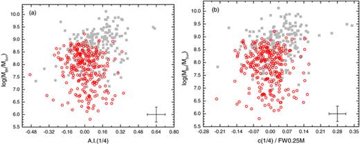
Population A and B sources (open circles and solid squares, respectively) are shown in plots of BH mass versus asymmetry index A.I.(1/4) (panel a) and normalized centroid shift c(1/4)/FW0.25M (panel b). In each panel, we also indicate typical 2σ error bars.

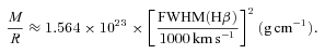
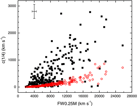
For N= 249 sources that show a positive centroid shift c(1/4), we plot that measured shift (solid squares) and the predicted gravitational redshift (open circles) versus the FW0.25M. We also indicate the typical 2σ error bars for the measured values of c(1/4).
A pertinent argument in favour of a separate and distinct emitting region is the existence of clear inflections on the red wings of the Hβ profiles in many individual sources (see for example the case of B2 1721+34 in Corbin 1997). In Fig. 16, we show an interesting case, SDSS J230443.47−084108.6, for which we have available recorded spectra at two different epochs, about eight years apart. The top panel shows the spectrum of the Hβ region observed in 1993 May (Marziani et al. 2003a) and the bottom panels show the Hβ and Hα spectral regions of the same source, provided by SDSS, observed in 2001 December. Not only do we see a significant change in the functional shape of the Balmer profiles, but we note the dramatic change on the red side of these lines. In the SDSS spectrum, we see a clear inflection on the red wing of both Hβ and Hα (see also the detailed monitoring study and complex behaviour of NGC 4151 as presented in Shapovalova et al. 2009). In many other cases, an inflection between the two components BLR and VBLR may or may not clearly show up in the line profiles. The two components may be structured differently and apparently they do not respond in tandem to the variations in the continuum (see the interesting case of PG1416−129 in Sulentic et al. 2000c), nor do they respond similarly to luminosity variations (Marziani et al. 2009). The search for a clear inflection on the Hβ red wing is further complicated by two additional emission features: (i) optical Fe ii has a non-trivial contribution in this region especially due to its multiplet m42 components and (ii) possible contamination by He i broad permitted emission lines that may contribute to the build-up of a red-shelf for both Hβ and Hα (Véron et al. 2002), as mentioned earlier.
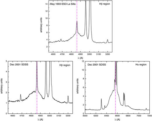
SDSS J230443.47−084108.6 observed at two different epochs. We note the change in the functional shape of the Balmer Hβ line wings. For the more recent records (lower panel), we show both the Hβ and the Hα regions. The vertical lines indicate the rest-frame Balmer wavelength positions. The ‘red shelf’ is clear in the later observation, especially in the Hα region. An inflection along the red wing of the Balmer lines may be a transient feature due to the variability of the emitting source.
However, the presence/absence of inflections is not necessarily offering us a definitive answer for or against multiple components of the broad lines. The inflections are sensitive to kinematics and/or orientation.
4.2 Disc wind
The blue asymmetry/blue-shifted signature in high accretors (Population A sources) could indicate an additional wind contribution. In such highly accreting sources, the presence of radiation driven winds is very likely (e.g. King & Pounds 2003; Komossa et al. 2008). We note that this potential second contribution on the blue wing of Hβ becomes more clearly inflected relative to the classical BLR when the [O iii] lines are weak and show a significant blueshift, too (see the examples in Fig. 5, where the [O iii] shift is indicated and see also the more extreme case shown in Fig. 17, where the [O iii] blueshift is ≈1500 km s−1 and the inflection on the blue wing of Hβ is unquestionable). A kinematic linkage between the [O iii] lines and the HIL line C iv blueshift was suggested by Zamanov et al. (2002). The same kind of linkage may exist between the [O iii] lines and the LIL Balmer lines. This idea is further reenforced by our Fig. 18. We show that there is a correlation between the shift of C iv (rest-frame λ1549 Å) at 1/2 fractional intensity and the normalized shift of Hβ at 1/4 fractional intensity (see also similar comparisons in Marziani et al. 1996). The data in the plot represent the common set of sources of the current sample of SDSS quasars and the sample explored spectroscopically in Sulentic et al. (2007). Although the size of the overlapping sample is rather small (n= 25) there is an important observation: there is no source showing a C iv redshift and an Hβ blueshift. We also note that a comparison between the Atlas presented in Marziani et al. (2003a) for the Hβ and the sample presented in Sulentic et al. (2007) for C iv reveals an overlap of n= 87 sources. 69 of those sources (∼80 per cent) show a shift of C iv that is larger than the shift in the Balmer line (at both 1/4 and 1/2 fractional intensity). This kind of empirical evidence suggests that the blue asymmetry/shift of Hβ might be produced by the same mechanism that is responsible for C iv shift, and the simplest interpretation may be a wind/outflow (e.g. Murray et al. 1995; Kollatschny 2003; Young et al. 2007).
![An extreme case that shows a clear inflection on the blue wing of Hβ accompanied by a −1500 km s−1 blueshift of [O iii]λ5008 Å. The vertical lines indicate the rest-frame positions for Hβ 4862.7 Å and [O iii] 5008.2 Å.](https://oup.silverchair-cdn.com/oup/backfile/Content_public/Journal/mnras/403/4/10.1111_j.1365-2966.2009.16236.x/1/m_mnras0403-1759-f17.jpeg?Expires=1750251562&Signature=PPEtIdyOll5i6VpjOfxpMpNr9euRblNHEzLaP8P3kc0C1-kcCmM20TFvfjuGTFLZAxHENb7U9QAAcHIntk~8YSXcOCKMb3UmZCJ-Cm8uFXjkp2~TNvLORlMmuRbwacH14G79jLRO320lWEsI8H5Z~YRAaL~jTn5ranz4Wkb4TQZE~rPPDbVkx5ed942bybdgIG-6md3SNbL~xe8Klc~KVxqztw~RGi8wlxLFOl7z3Sv9MVUWk~y0E78Phoza5502KuHRGQ-MawKvj732sPsVC~NiU~gnzjTe5McT1HrHNSnKwGrUDK93DGW5WO5HFFkampj7qN9bbaMO7TV4x67QTg__&Key-Pair-Id=APKAIE5G5CRDK6RD3PGA)
An extreme case that shows a clear inflection on the blue wing of Hβ accompanied by a −1500 km s−1 blueshift of [O iii]λ5008 Å. The vertical lines indicate the rest-frame positions for Hβ 4862.7 Å and [O iii] 5008.2 Å.
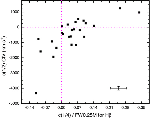
A comparison between the C ivλ1549 Å and Balmer Hβ shift. Data shown represents the overlap between the current sample and the sample of quasars examined in Sulentic et al. (2007). The dotted lines indicate the zero shift for C iv (vertical axis) and Hβ (horizontal axis). Typical 2σ uncertainties are indicated.
The shift of quasar broad emission lines (relative to their rest frame) has been intensively studied (e.g. Gaskell 1982; Wilkes 1984; Carswell et al. 1991; Tytler & Fan 1992; Corbin 1995; McIntosh et al. 1999; Vanden Berk et al. 2001; Richards et al. 2002). It has been reported that the amplitude of the shift is correlated with the ionization potential (e.g. McIntosh et al. 1999; Vanden Berk et al. 2001). The aforementioned comparison between the shift of the Hβ and C iv (based on the Atlas of Marziani et al. 2003a and the sample of quasars from Sulentic et al. 2007) supports it.
4.2.1 Other arguments for the wind scenario
Kallman & Krolik (1986) argued that when HILs are systematically blueshifted relative to the quasar's rest frame by thousands of km s−1 it becomes more likely that absorption lines with zabs > zem will exist. Let us examine the concrete case of quasar PG 1700+518, which shows both low- and high-ionization absorptions (Pettini & Boksenberg 1985; Laor & Brandt 2002) and a clearly blue-asymmetric Hβ profile (Marziani et al. 2003a). Young et al. (2007) offer arguments in favour of a strong rotating wind in this source. This scattering wind rises nearly vertically from the disc over a range of radii approximately coincident with the Balmer emitting region. So, the assertion of Kallman & Krolik (1986) could be extended to the blueshifted components of LILs like Hβ, i.e. when sources show large blue-asymmetries in the Balmer emission lines, the BAL signatures in Mg iiλ2800 Å or C ivλ1549 Å could be present as well. In the case of PG 1700+518, it is also possible that we see the BLR disc more face-on than equatorially (Richards et al. 2002) and the blue-asymmetry is formed by scattering in a wind outflow. Another similar case studied in detail is IRAS 07598+6508 (Lipari 1994; Véron-Cetty et al. 2006). This source shows both Mg ii and C iv BAL signatures and an inflected blue wing of the Hβ emission line. Both quasars mentioned here have been interpreted as examples of nuclear young/starburst (IRAS 07598+6508) or post-starburst (PG 1700+518) by Lipari (1994).
Exploiting the analogy between microquasars, stellar-scale phenomenal and quasars, galactic-scale phenomena, one can also interpret the recent study Neilsen & Lee (2009) as supportive for the idea that the presence of disc winds inhibits the formation of jetted radio structures. This may have implications for the fact that FR ii quasars and sources where disc wind signatures are more evident occupy mutually exclusive regions in the optical plane of the 4DE1 parameter space.
4.3 Other scenarios for the shifted broad lines
Richards et al. (2002) offer a different view on the matter of the C iv blueshift. They propose that the blueshift is an apparent effect produced by obscuration of the redshifted photons. In the proposed scenario, the largest blueshifts (which may not be real, but rather due to the lack of flux in the attenuated red wing) are explained by an equatorial viewing angle of the line emitting region(s). An argument of Richards et al. (2002) that favours an equatorial view of the BLR when we observe increasingly larger blueshifts of the HIL like C iv is that the composite spectrum of the most blueshifted C iv spectra is most similar to that of BAL quasars. This similarity would indicate that the red wing of C iv is attenuated by obscuring material. Another argument raised in favour of obscuration coupled with orientation (external or internal) is the finding that the strength (equivalent width) of the C iv line declines with increasing blueshift. This is difficult to reconcile with the Fe ii emission that is likely produced in a high density/column density environment (flattened geometry; e.g. Collin-Souffrin et al. 1988a). We do observe that the average strength of the Hβ broad emission line declines by a factor of 2 from A1 to A4 [Figs 1(b) and (c)] and the Hβ blue asymmetric and blueshifted base is typical for bins A/4 [lower equivalent width W(Hβ)], however, this can be explained by a quenching of the Balmer emission in high electron density environments (Gaskell 2000), which favour the Fe ii emission [as we see in Figs 1(b) and (c), W(Fe ii) increases by the same factor of 2 from bin A1 through bin A4). Largest blueshifts correspond to narrowest and strongest Fe ii, and we suggested that Fe ii decreases from face-on because of a sort of ‘limb darkening’ (Marziani et al. 1996), which supports a wind scenario plus disc obscuration, but a different orientation dependence from the one suggested by Richards et al. (2002): the largest blueshifts are observed when the source is viewed pole-on.
Richards et al. (2002) advocate the ubiquity of the C iv blueshift. This last result is not confirmed by the most recent study of Sulentic et al. (2007), where only Population A quasars show such a spectral signature. Population B sources (where the majority of RL quasars belongs) show unshifted and symmetric C iv profiles. Most likely the bins of least C iv blueshift in Richards et al. (2002), which also have the largest radio-detected fraction and the largest C iv equivalent width (see their table 2), must have a significant overlap with the Population B sources. It is difficult to see how attenuation of the C iv red wing, according to the orientation dependence suggested by Richards et al. (2002), can leave a symmetric profile in so many quasars: Population B sources account for ∼60 per cent of our C iv sample (Sulentic et al. 2007).
An alternative to the wind interpretation of blueshifts was recently proposed by Gaskell & Goosmann (2008). They advocate that the blueshift of HIL like C iv is produced by Rayleigh and/or electron scattering off of inflowing material of the BLR. Their model predicts that the relative blueshifts of different lines in the same AGN should be proportional to the inverse square root of the radius where they are produced. The results we indicated in the previous paragraph, that the Hβ blueshift is almost always less than that of C iv are consistent with the prediction of Gaskell & Goosmann (2008) in the sense that C iv is probably emitted at a smaller radius within the BLR relative to the Balmer emitting region. This is qualitatively supported also by the fact that HIL C iv line shows broader FWHM profiles than Hβ in Population A sources (but not in B; see Sulentic et al. 2007). Moreover Gaskell & Goosmann (2008) predict the amplitude of the blueshift is proportional to the infall velocity. Spectroscopic signatures of the inflow have been indicated (see section 2.1 of Gaskell & Goosmann 2008; see also Bentz et al. 2008), although very recent reports (Denney et al. 2009; Shapovalova et al. 2009) indicate evidence for a very diverse behaviour of the BLR, which can show signatures of outflowing, inflowing and virialized gas motion in different sources.
If the scattering effect depends on the wavelength only, then low-ionization lines in UV should show a blueshift comparable to that of the UV high-ionization lines. Published data Tytler & Fan (1992) as well as a tentative analysis on several Hubble Space Telescope spectra (Negrete et al., in preparation) do not support this suggestion. The OI1304 Å for example, does not seem to show the large blueshift of C iv and seems to be more consistent with the quasar rest frame as derived from the narrow low-ionization emission lines.
Recently, Hu et al. (2008a,b) propose that inflow may be a ubiquitous phenomenon as revealed by their measured (red-) shift of the Fe ii optical lines. However, Hu et al. (2008a,b) report that the infall is increasingly pronounced as the accretion rate (or Eddington ratio) decreases. This works against the model proposed by Gaskell & Goosmann (2008) because the largest blueshifts are typically observed in highly accreting sources (members of the Population A). The Hu et al. (2008a,b) recent papers propose that there is an intermediate line region (ILR) component in Hβ that is systematically redshifted and narrower than a so-called VBLR rest-frame component. This is a rather different view compared to the proposed two-component model of Sulentic et al. (2002) or Marziani et al. (2009), where the VBLR shows a significant and systematic redshift and the classical BLR signature is basically at the quasar's rest frame. A two-component model employing the VBLR/ILR terminology is proposed by (Popović et al. 2004), where the emission of the line wings comes from a disc and the line core from a distinct emitting region that has spherical geometry. The two emitting regions may be linked by a wind. One must be cautious about different definitions and labels of the broad line emitting regions used by different studies; the same name may be assigned to different structural components.
We are not yet convinced of the ubiquity of the Fe ii redshift proposed by Hu et al. (2008a,b). Although we do not dismiss that in sources like SDSS J094603.94+013923.6 or SDSS J101912.57+635802.7 (both shown in Fig. 5) the Fe ii could be redshifted, we also encounter sources like SDSS J001224.02−102226.54 or SDSS J094756.00+535000.3 that can be difficult to fit in the scenario they propose. We also find an excess of blueshifted peaks in both Populations A and B, which does not support the idea of a redshifted ILR in virtually all quasars. This is further confirmed by the composite spectrum shown in Fig. 4 for bin B2, which should show a significantly redshifted Fe ii signature, which we do not see. Moreover, we selected the (apparently) brightest sources in their sample (psf i or psf g < 17.5, just as we constrained our SDSS low-z sample; Zamfir et al. 2008). We found about 50 such sources with a claimed Fe ii redshift larger than 1000 km s−1. The authors state that their sources are bright enough that the host galaxy plays a negligible role. We did find sources where prominent absorption lines indicate a host galaxy contamination, e.g. SDSS J110538.99+020257.3. This raises the question whether the mismatch between the Fe ii rest-frame template and the spectral lines is severely affected by the dips created by an ignored host galaxy signature. The problem has profound implications towards understanding the link between the 4DE1 space (through RFe ii) and its proposed main driver Lbol/LEdd (see the very recent study of Ferland et al. 2009) and thus requires further scrutiny.
4.4 The relative fraction of population A/B
Shen et al. (2008) compile BH masses for 60 000+ Sloan quasars within redshift z= 4.5, starting from the catalogue of Schneider et al. (2007), which imposes a faint limit of −22 for the absolute i-band magnitude. In order to compare to our sample, we selected from Shen et al. (2008) (using the VizieR catalogue data base, Ochsenbein, Bauer & Marcout 2000) only the quasars with z < 0.7. There are 12 003 listed sources, of which 8979 have reported measurements of the Hβ line. We were unable to understand why ∼25 per cent of the sample has no reported measures of Hβ. They are neither fainter nor noisier/more problematic spectra than the rest. The other major criticism is the relative proportion of sources that we would call A/B in the light of our adopted 4000 km s−1 boundary. They report 71 per cent sources with FWHM(Hβ) > 4000 km s−1 (of those 8979 measured). We tested whether and how this proportion is tied to the S/N reported by their study. We found that as the S/N decreases there is an increased fraction of Population A sources (i.e. 19 per cent for S/N > 20, 26 per cent for S/N > 15–20, 30 per cent for S/N > 5–15). All previous major studies of quasars in the context of Eigenvector 1 space (e.g. Boroson & Green 1992; Sulentic et al. 2000a,b; Marziani et al. 2003a) report a slight numerical dominance of Population A sources (at low z), i.e. FWHM(Hβ) < 4000 km s−1. Our main concern is their adopted Hβ fitting routine, i.e. a single Gaussian for all profiles. We now know that Population A spectra are best described by Lorentz profiles, while for Population B sources is a double-Gaussian model works better, due to their pronounced red asymmetry (Sulentic et al. 2002; Netzer & Trakhtenbrot 2007; Marziani et al. 2009). A single Gaussian fit would overestimate the FWHM measure in both Population A and B sources; for instance a single Gauss fit to the A2 or B1 bin median composites spectra (discussed earlier in Section 2.4) would overestimate the FWHM of the broad Hβ by 20–25 per cent. Another serious problem with their analysis is the inclusion of a large number of spectra of sources that are either in a high-continuum phase or the emission lines are intrinsically very weak (e.g. SDSS J083353.88+422401.8, SDSS J083148.87+042939.0), where the broad lines are almost missing. For such cases, they report hugely overestimated values of the FWHM(Hβ).
5 CONCLUSIONS
We have shown that the Population A/B concept proposed in the context of the 4DE1 Parameter Space holds robustly when other line diagnostic measures like centroid shifts, asymmetry and kurtosis are considered. Taken at face value the spectral measures tell us that populations A/B show a great deal of difference in terms of BH mass and Eddington ratios (Fig. 10). This may be indicating that the numerous observed dissimilarities between A and B are indeed driven by large differences in the structure and kinematics of the central engine. None the less, large differences in terms of BH mass and Eddington ratio may be reduced. On one hand, it was pointed out that NLSy1 sources may not harbour such small BH masses as inferred from their narrow emission lines. They might not be super-Eddington accretors if proper correction for radiation pressure (Marconi et al. 2008, 2009; but see also Netzer 2009), orientation (Marziani et al. 2003b; Decarli et al. 2008) and geometry (e.g. Collin et al. 2006) are made. On the other hand, if the Hβ profiles that show a large red asymmetry, which is probably caused by a distinct VBLR redshifted contribution, are properly corrected for such ‘unvirialized’ contributions, then the estimated BH mass gets smaller and thus the measured Eddington ratio gets higher. The large variance of the 4DE1 space would be significantly reduced from both sides of the accretion rate sequence. As a consequence, the FWHM measure, which is an important optical dimension within 4DE1, may be replaced with A.I.(1/4) or the normalized c(1/4)/FW025M centroid shift. They correlate at least equally well with RFe ii (Fig. 9). None the less, incorporating these two new measures in the 4DE1 is not an easy task, as they also manifest (at least in Population B) a sensitivity to luminosity (Netzer & Trakhtenbrot 2007; Marziani et al. 2009), which was indicated as part of the Eigenvector 2 space (Boroson & Green 1992), formally orthogonal to Eigenvector 1. Moreover, the Population B Hβ asymmetry/centroid shift at the base (1/4 fractional intensity) appears weakly correlated with the BH mass (Fig. 14; see also Marziani et al. 2009).
We also presented several arguments that two populations of quasars may be redefined based on an RFe ii nominal boundary of 0.50. This could be seen as an alternative empirical definition of some equivalent Populations A and B. The lines of evidence are as follows: (1) RFe ii= 0.50 seems a critical value that best isolates RL quasars from the rest of quasars (recall fig. 4 from Zamfir et al. 2008), (2) around this measured value of RFe ii the centroid shift and the asymmetry of Hβ change sign [Figs 9(a) and (b)], (3) a plot of the line shape kurtosis index K.I. versus RFe ii shows two different trends on either side of RFe ii∼ 0.50 [Fig. 9(c)], likely separating low from high-accreting sources [Fig. 12(d)] and (4) a tight correlation between RFe ii and the Eddington ratio indicates that RFe ii∼ 0.50 roughly corresponds to Lbol/LEdd∼ 0.18[Fig. 9(d)], consistent with several other studies that suggest a critical change in the structure/geometry/kinematics in the quasar ‘engine’ around that value. The red and blue Hβ base asymmetries observed at the opposite ends of the Eddington ratio sequence may have very different origins.
We also find that our measures for low accretors (typically members of Population B) seem to match the predictions of accretion disc models, i.e. blueshifted peaks c(9/10) and redshifted/red asymmetric bases c(1/4) and A.I.(1/4) [Fig. 12(b)]. This allows us to suggest a typical flattened BLR geometry for all Population B quasars, not only for the RL quasars, whose majority is seen in Population B subspace. We emphasized that our conclusions are not driven by radio-loudness. Focusing our investigation on the RQ subsample, the results are similar to what we get using the whole sample of N= 469 quasars.
Although the sample of FR ii sources is relatively small (N= 44), we find a very interesting correlation between the core:lobe flux density ratio, which may be seen as an orientation indicator (based on the 1.4-GHz Faint Images of the Radio Sky at Twenty-Centimeters (FIRST) survey measures) and the redshift of the Hβ base (Fig. 19). The more core-dominated FR ii sources show a more pronounced redshift at 1/4 fractional intensity (see also Figs 9(a) and (b), and related commentaries). We may just speculate that the excess of redshifted photons could be a signature of an inflow feeding the central mass and allowing for a jetted burst.5 A larger sample should be investigated.
Assuming that the true parent population of RL quasars are FR ii sources there should exist for every core-dominated RL source of a certain radio luminosity an even weaker radio power FR ii, if the unification scenario is valid.
A recent study Nikołajuk, Czerny & Gurynowicz (2009) postulates that ‘the division between NLSy1 and BLSy1 based on the width of Hβ line is less generic than according to the soft X-ray slope’, which actually is one of the four adopted dimensions of the 4DE1 space.
A similar case SDSS J153636.22+044127.0 was found in SDSS DR7 by Boroson & Lauer (2009) and interpreted as a possible signature of a sub-parsec binary BH system. Although a number of other articles propose alternative explanations.
See the interesting case of the micro-quasar GRS1915+105 presented by Neilsen & Lee 2009. Their study suggests that accretion disc winds prevent the jetted outbursts and vice versa.
Funding for the SDSS and SDSS-II has been provided by the Alfred P. Sloan Foundation, the Participating Institutions, the National Science Foundation, the U.S. Department of Energy, the National Aeronautics and Space Administration, the Japanese Monbukagakusho, the Max Planck Society, and the Higher Education Funding Council for England. The SDSS Web Site is http://www.sdss.org/. The SDSS is managed by the Astrophysical Research Consortium for the Participating Institutions. The Participating Institutions are the American Museum of Natural History, Astrophysical Institute Potsdam, University of Basel, University of Cambridge, Case Western Reserve University, University of Chicago, Drexel University, Fermilab, the Institute for Advanced Study, the Japan Participation Group, Johns Hopkins University, the Joint Institute for Nuclear Astrophysics, the Kavli Institute for Particle Astrophysics and Cosmology, the Korean Scientist Group, the Chinese Academy of Sciences (LAMOST), Los Alamos National Laboratory, the Max-Planck-Institute for Astronomy (MPIA), the Max-Planck-Institute for Astrophysics (MPA), New Mexico State University, Ohio State University, University of Pittsburgh, University of Portsmouth, Princeton University, the United States Naval Observatory and the University of Washington.
This research has made use of the NASA/IPAC Extragalactic Data base (NED) which is operated by the Jet Propulsion Laboratory, California Institute of Technology, under a contract with the NASA. This research has made use of the VizieR catalogue access tool, CDS, Strasbourg, France.
REFERENCES
