A fast computation of the secondary ion production in the ionosphere of Mars

Abstract

1 INTRODUCTION

Present-day observation of the Martian ionosphere continues to reveal new and interesting phenomena. Studies have highlighted features that are similar to those of other planetary ionospheres and features that are specific to the Martian plasma environment. In discussion of the former, one can draw upon examples such as the similarities in ionic constituents between the Venusian and Martian ionospheres (Witasse et al. 2008), or the occurrence of auroral phenomena in the upper atmospheres of Mars, Earth and the giant planets (see Bertaux et al. 2005). In the latter case, the unique Martian magnetic topography, typified by the crustal magnetic fields, has a very complex structure and creates so-called ‘mini-magnetospheres’ that manipulate the solar wind interaction downwards into and horizontal convection across the Martian ionosphere (Breus et al. 2005). Additionally, comparison of ionospheric similarities and differences at several Solar System ionospheres due to the same phenomena experienced at multiple planets provide constraints to our knowledge not possible by the study of only a single upper atmosphere. Take for example the enhanced solar high energy X-radiation experienced successively at Earth, Mars, Jupiter and Saturn due to a single specific solar flare event (Mendillo et al. 2006). This allowed the effects of solar flux variation to be studied in isolation away from slower changes in neutral atmosphere variation.

As revealed by the Retarding Potential Analyzer (RPA) instruments onboard the two Viking landers (Hanson et al. 1977) the major ion in the Martian ionosphere is O⁺₂, with a peak density of approximately 10⁵ cm⁻³ at an altitude of 130 km. Both CO⁺₂ and O⁺ were also detected. Peak densities for these latter two species are approximately 10⁴ cm⁻³ at 140 km and 8 × 10² cm⁻³ at 230 km, respectively (Witasse et al. 2008). Although the RPA instruments made the first ever in situ ionospheric measurements of a planet other than the Earth (Nagy et al. 2004), our knowledge of the Martian ionosphere remained incomplete for a period of 20-yr before the Mars Global Surveyor (MGS) and more recently the Mars Express missions returned with radio science, electron reflectometer and magnetometer instruments to continue observational study. As a consequence, an extensive set of electron density profiles has been collated from the aforementioned missions, adding to results from Mariners 4, 6, 7 and 9, Vikings 1 and 2 and Mars 4 and 5 missions (Nagy et al. 2004).

Electron density data from the pre-MGS missions were studied collectively by Zhang et al. (1990) and revealed that, about the peak, the Martian ionosphere is fairly well described by ideal Chapman theory. Thus, the peak density shows a close cos^1/2χ dependence (where χ is the solar zenith angle) with a photochemical equilibrium being quickly established between production and loss of electrons (Bougher et al. 2001). Likewise the altitude of the peak, when acting under the local control of photochemical processes, depends upon how deeply the solar radiation penetrates into the atmosphere. The ionosphere also showed a notable degree of consistency in the typical electron density profile structure about the region of the peak (it is altitude and magnitude) and the scaleheight exhibited up to approximately 200 km. Further modelling work confirmed that the dayside ionosphere, below approximately this altitude, is not subject to vertical or horizontal transport of ions (e.g. Bougher et al. 2001).

Electron density data have been used post-MGS to study the interannual variability of the ionosphere and as a proxy to study neutral atmospheric phenomena such as solar-driven tides by considering the occurrence of those same phenomena in the ionosphere (Bougher et al. 2001, 2004; Cahoy et al. 2006; Hinson et al. 2007). Both MGS and Mars Express have also highlighted the complexity of the Martian magnetic field and energetic electron fluxes of the near-Mars space environment (Krymskii et al. 2003; Withers et al. 2005; Soobiah et al. 2006). More recently, studies using UV and IR spectrometer data from the Mars Express SPICAM instrument (Simon et al. 2008), including comparison of intensity profiles of the Cameron CO bands and CO⁺₂ UV doublet at 289.0 nm, have helped to continue to reveal the underlying ionospheric and neutral atmospheric conditions (e.g. density and temperature).

The adherence or otherwise of the Martian ionosphere to Chapman theory and the close dependence on the neutral background atmospheric structure and solar UV/EUV/X-ray radiation has been intensively analysed, modelled and summarized by many authors in one, two and three dimensions using kinetic, fluid, hybrid and MHD mathematics (see for example Fox 2004 and references in Nagy et al. 2004; Wang & Nielsen 2004). However, despite these advances much remains to be learnt about the Martian ionosphere (in-situ ion measurements e.g. remain especially limited). The topside Martian ionosphere and its interaction with the solar wind, the effect of the crustal magnetic fields on the ion and electron dynamics & energetics and finally the description of the night side ionosphere all remain as perhaps the most challenging areas for further study.

In this paper, we look at the relationship between primary photoproduction (i.e. through photoabsorption) and secondary electron impact production (i.e. through energetic electron propagation). The computation of ion and electron densities by primary photoproduction is straightforward and fast, however the ionic production by energetic electron propagation through the background neutral atmosphere and subsequent electron impact is a far more involved and complex computation. Thus, we provide a method by which the secondary ion and electron production can be rapidly calculated by using the production efficiency (ε, defined as the ratio between the secondary and primary productions) as an intermediary. Our use of the production efficiency is advantageous not only for the swift computation of production rates it affords us but also because it will reflect changes in both the primary and secondary production rates, which in turn will be due to any variation in the background neutral density (Forget et al. 2009) due to orbital and solar cycle conditions. Of course, these can be studied by using our three-dimensional global circulation model.

The layout of this report is as follows. In Section 2, we describe individually the two models used for our study, Trans-Mars and Mars Thermosphere and Ionosphere Model (MarTIM). In Section 3, we describe the rapid computation method. Finally, we discuss the applicability of our results to various solar and seasonal conditions in terms of how the variation of the neutral background atmosphere affects our results.

2 PRODUCTION COMPUTATION

Our study was conducted using two recently coupled models of the Martian atmosphere. The first model is a one-dimensional kinetic electron transport code developed at Laboratoire de Planétologie, Université Joseph Fourier/CNRS, Grenoble that solves a stationary Boltzmann equation for the energetic electron flux. It belongs to the Trans-* family of models that have been, over recent years, applied to describe the ionospheres and planetary upper atmospheres of Earth, Venus, Titan and Mars (see Lilensten & Blelly 2002; Gronoff et al. 2007, 2008; Galand et al. 1999; Witasse 2000, respectively). The term Trans-* is shorthand for ‘transport’ as in the transport of energetic electrons through an atmosphere. The second model is a three-dimensional global circulation model of the neutral Martian atmosphere developed at the Atmospheric Physics Laboratory, University College London. It goes by the acronym MarTIM, which stands for MarTIM. MarTIM's basic model core was provided by a global circulation model of Titan's neutral atmosphere (Müller-Wodarg et al. 2000), which was converted to describe the Martian thermosphere and ionosphere by Moffat (2005). Most recently MarTIM was used to study the coupling between the lower and upper atmospheric regions of the Martian neutral atmosphere (for solar minimum conditions) (Moffat-Griffin et al. 2007). When these two models work together we refer to the coupled code with the name Trans-TIM.

2.1 The kinetic electron transport model

The kinetic part of Trans-TIM distinguishes between two subpopulations of electrons present in the Martian ionosphere, based on the influence they have on the physics of the ionosphere; the thermal electrons and the suprathermal electrons. In this study, we model the propagation and degradation in energy and altitude of the suprathermal electrons as they propagate through the Martian neutral and ionic background atmosphere. The principal source of suprathermal electrons for the kinetic code in this study is the solar-produced photoelectrons with a calculated dependence on solar zenith angle, solar activity and solar longitude. Alternative precipitated sources from available plasma observations (e.g. Acuña et al. 1998) can also be used as an upper boundary condition if desired allowing, for example, the creation of the Martian night side aurora from the influx of auroral electrons to be studied (see Bertaux et al. 2005) or indeed the intricate night side ionospheric structure (Fillingim et al. 2007). In any event, we refer to these as ‘primary’ electrons and model the ionization, excitation and heating caused by their propagation and collision with the ambient atmosphere. Though note again we only study solar produced photoelectrons in this report.

The thermal electrons are simply a component of the ambient background and thus the distinction between the two electron populations centres upon a ‘cross-over’ or ‘thermal’ energy defined [in (eV)] as E_t=k_BT_e, with k_B= 8.61 × 10⁻⁵ (eV K⁻¹), the Boltzmann constant and T_e the temperature (K) of the ambient electrons (Swartz et al. 1971; Lummerzheim & Lilensten 1994). We assume the electron distribution is dominated by thermal electrons below E_t and by the streaming suprathermal electrons above E_t. Heating of the ambient thermal electrons occurs either by a continuous friction-like term [the loss function L(E), see equation 4] representing energy loss to the thermal electrons at all energies or when primary electrons degrade in energy into the thermal energy range. Ionization events caused by inelastic collision between primary electrons and neutral components of the ambient atmosphere produce ‘secondary’ ions and electrons. It is the ratio of these secondary ions and electrons to their primary counterparts that we call the production ‘efficiency’ (ε). However, since the computation of primary electron collision processes and the production of secondary ions and electrons is far more complex than the primary photoionization calculation alone. Our aim is to provide a method that uses the production efficiency to rapidly calculate all ionic components of the Martian ionosphere.

The kinetic model describes the ionosphere using a fixed altitude grid ranging between 80 and 500 km and an energy grid ranging between 0.1 and 280 eV. The energy range is divided into 40 grid points whose spacing is non-uniform and determined by a power law. This type of energy grid means that the energy step between successive energy grid points increases with energy and thus the lowest energies are described with a finer resolution. This is advantageous as theory would suggest (Ratcliffe 1972) that all charged particles ionize most rapidly near the ends of their paths through the atmosphere before they return to the thermal (ambient) electron background. Thus, the ionization is most prominent when the time spent by a primary electron near a background atom is comparable with the period of a thermal electron in a Bohr orbit about that background atom. With a fine energy grid we can take this into account.

In studies of the terrestrial atmosphere and ionosphere using the Trans-* suite of kinetic models, the z-axis is held as vertical and modelling is restricted to polar regions, where primary electrons are guided vertically into the atmosphere by the geomagnetic field. With a vertical magnetic field strong enough to impose a negligible Larmor radius, we can assume an axial symmetry around the field line. In turn, this removes any dependence on the horizontal coordinate as long as we further assume that the atmosphere is locally horizontally stratified and that photoproduction is isotropic, both reasonable assumptions. Such considerations can also be applied to a study of the Martian atmosphere on the assumption that either (1) we are at the edge of one of the Martian anomalies such that a strong magnetic field is aligned vertically or (2) the induced magnetic field is sufficiently diffused over the region from the upper atmosphere to the altitude of the ionospheric peak (where our study is most concerned) such that its influence on the electron and ion trajectories can be neglected or (3) there is no magnetic field at all, such as would likely be experienced away from the localized magnetic anomalies associated with the crustal magnetic fields.

With the above assumptions considered the transport equation can be written as (Stamnes & Rees 1983)

1

where: Φ(τ, E, μ) is the stationary electron flux (cm⁻² s⁻¹eV⁻¹ sr⁻¹),

• ∂τ(z, E) is the electron scattering depth,

• z is the altitude,

• μ, μ′ are the cosines of scattered and incident electron pitch angles,

• E and E′ are the energies (eV) of scattered and incident electrons,

• n_k(z) and n_l(z) are the number densities of neutral species k and l at altitude (z),

• n_e(z) is the thermal electron number density at altitude (z),

• R_l is called the redistribution function and describes the degradation from a state (E′, μ′) to a state (E, μ) for the neutral l,

• σ^T_k(E), σ^T_l(E) are the total collision cross-sections (elastic plus inelastic) for the neutrals k or l for a colliding suprathermal electron of energy (E).

The second term on the right-hand side of equation (1) is the primary photoelectron source term (cm ⁻² s⁻¹ eV⁻¹ sr⁻¹) due to either the solar EUV flux or precipitated into the upper modelled atmosphere. For this study, we restricted our primary electron source to be only the solar photoelectron source,

2

where q_k,i(z, E) is the primary photoelectron production rate (cm⁻³ s⁻¹ eV⁻¹) and is equal to

3

where the relationship between the photon energy E_hν and the suprathermal electron energy grid is accounted for, with the statement E_W=E_hν−I_k,i. Thus, we take the difference between the energy E_hν of the incident solar photon and the ionization threshold I_k,i of species k and state i to calculate the energy of our created photoelectrons (E_W). Then, we simply ensure that the energy E_W is associated with the correct suprathermal electron energy grid position E, i.e. we use the former to search through the latter to build our source function upon energy grid E. For the other terms, we have:

• σ^ion_k,i (E_hν) photoionization cross-section for species k, state i for photon energy E_hν;

• I_∞(λ_hν) solar EUV flux at the upper boundary of the atmosphere and

• σ_m(E_hν) photoabsorption cross-section of neutral species m for photon energy E_hν.

Finally, regarding the second term, note how the primary photoproduction is calculated by considering a column of atmosphere along the line of sight of the solar photon beam by using the Chapman function provided by Smith & Smith (1972) to describe high solar zenith angle (χ) grazing incidence. The Chapman function depends upon both the scaleheight and the radial distance from the centre of the planet to the point in question (R_M+z). For the radius of Mars term (R_M), we require a description of Mars global surface shape. Since the Martian areoid will vary with latitude and longitude due to local topographic features, we follow the procedure used by the Mars Climate Data base (Lewis et al. 1999) and approximate its shape by an offset spheroid whose characteristics can be found at http://ssed.gsfc.nasa.gov/tharsis/geodesy.html. Thus, zero elevation (from which our altitude z is measured) is defined as the equipotential surface whose average value at the equator is 3396 000 m (after Smith et al. 1999). Although this means that the polar radius is approximately 20 000 m less than the equatorial radius we would not expect this difference to introduce any significant variation in our calculation of the Chapman function were we instead to approximate Mars' shape by a sphere of radius 33 96 000 m. For the various values of scaleheight used, we note that this depends upon the particular background neutral atmosphere calculated. Thus, we refer the reader to the description of our neutral atmosphere model in Section (2.2) for more details.

The loss function L(E) was introduced earlier as representing a continuous friction-like term responsible for energy loss from the precipitating energetic suprathermal electrons to the ambient thermal electrons. We assume that the primary electrons are not deflected in this process (Blelly et al. 1996). In equation (1), it appears in the third term on the right-hand side. The full expression is (Swartz et al. 1971; Lummerzheim & Lilensten 1994)

4

This term requires self-consistently calculated profiles of electron temperature (T_e, for use in E_t=k_BT_e) and of background (thermal) electron density (n_e) to be provided. For the latter, we recall statements made earlier in the introduction that about the peak the Martian ionosphere is fairly well described by ideal Chapman theory. With this in mind, we use the formulation of Fox et al. (2006), equation (5), to describe the electron density input to the kinetic model as a function of solar zenith angle and altitude. In this formulation, the Chapman layer is defined as being produced by the photoionization of a single molecular species for which the resulting molecular ion is destroyed locally by dissociative recombination with a rate coefficient α_dr. Fox et al. (2006) adopt a value for α_dr of 1.95 × 10⁻⁷ (300/T_e)^0.7 cm³s⁻¹ for T_e < 1200 K and a value proportional to (300/T_e)^0.56 for T_e > 1200 K. Analysis of the resulting Chapman layer (see the solid line of Fig. 1) shows that for equinox conditions at heliocentric distance of 1.47 au for overhead sun conditions, and with our neutral background atmosphere, that the peak electron density reaches a value on the order of 10⁵ cm⁻³ at ∼125 km.

Figure 1

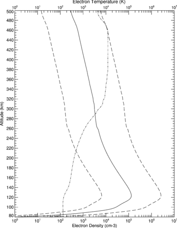
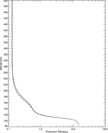
Electron density (solid line) profile (n_e) for the Sun overhead, equinox conditions. Also shown are variations in n_e investigated in preparation for this study (dashed lines, see text). Electron temperature (dot–dashed line) profile (T_e) used throughout this study (see text).

Open in new tabDownload slide

For the electron temperatures (T_e), unfortunately we are quite limited in our capacity to self-consistently calculate appropriate profiles and instead require the plasma temperatures to be provided as inputs to be read in directly to Trans-TIM either from other models or from available spacecraft data. For this study, then we take the profile calculated in the work of Witasse (2000) where a full fluid model component was coupled to the Trans* kinetic part. This fluid model component solved an eight-moment approximation to the Boltzmann's equation for the distribution function (see Blelly et al. 1996) appropriate to Viking conditions. The resulting electron temperature profile is shown by the dot–dashed line in Fig. 1.

We do appreciate the limitations that our choice of both the electron number density and electron temperature brings to the breadth of study we can present, while maintaining full self-consistency. However, we note that the frictional processes the loss term of equation (4) represents (including energy loss through Coulomb collision and Çerenkov wave generation) are more important at low energies (in particular less than the ionization threshold) and so are not expected to influence the secondary electron production (Galand et al. 1999). Consequently, since this study is focused squarely on the efficiency of ionization processes, that is the secondary to primary ionization relationship, we do not consider our choice of n_e nor T_e to limit in any way the range of conditions (solar zenith angle, solar activity, etc.) we can consider.

Indeed, we studied the effect of using two other electron density profiles as inputs to our coupled model. One with the Chapman layer profile multiplied by a factor of 20 and the other with it divided by a factor of 20 (see the dashed lines of Fig. 1). This factor was chosen by the following recent remote-sensing observations of the neutral CO₂ density using the SPICAM instrument onboard Mars Express (Forget et al. 2009) that revealed density varied annually by a factor of 20 at 120 km. Thus, we assume a like-for-like variation is possible in electron densities. In the efficiency profile results, which are not shown here, we found no discernible variation in the production efficiency and therefore feel confident that using the limited plasma inputs discussed throughout the rest of the present study will not affect any of our production efficiency results.

The last term on the right-hand side of equation (1) represents the electron production due to degradation of higher energy fluxes through collisions between primary electrons and neutral particles (Blelly et al. 1996). In this term, R_l is known as the redistribution function and is defined as the ratio of (in the numerator) the sum of differential cross-sections (sum of cross-sections over different elastic and inelastic collisions) between electrons and neutrals to (in the denominator) the total cross-section σ^T_l. The differential cross-sections are deduced from the collision cross-sections as described in Lummerzheim & Lilensten (1994). Collisions between secondary electrons are neglected.

The solution to the transport equation is formally equivalent to the equation of radiative transfer. The programs originally developed to solve the core of the kinetic model are described in Lummerzheim & Lilensten (1994), wherein the discrete ordinate method is adopted using the Discrete Ordinate Radiative Transfer (DISORT) procedure of Stamnes et al. (1988) where eight streams (or pitch angles; referring to the angle between the particle velocity and the vertical direction) are used as recommended by Lummerzheim & Lilensten (1994). In this ‘multistream’ approach, we must account for the energy distribution associated with and the angular dependence of secondary electrons generated by inelastic collision between primary electrons and the background atmospheric gases (Opal et al. 1971).

For the angular dependence, we assume that during an inelastic collision producing an ionization or excitation the incident primary electron is scattered mostly forward (Blelly et al. 1996) so that the collision phase function [which governs the angular redistribution of energy degraded primary electrons (Lummerzheim et al 1989)] can be approximated by a Dirac-delta function in the forward direction. We assume that the secondary electrons produced may be scattered in any direction, i.e. they are distributed isotropically. This was justified in the work of Lummerzheim & Lilensten (1994), whose study of the angular redistribution function for the secondary electrons showed that it had no influence on the altitude profiles of heating rates, energy deposition rates nor emission rates.

For the case of elastic collisions, the converse situation is apparent: results are sensitive to the phase function for elastic scattering (Lummerzheim et al 1989). We use the parametrization developed by Porter & Jump (1978) and Porter et al. (1987) for the angular redistribution and the required equation is

5

with the normalization N given by

6

Here Θ is the total scattering angle and Porter et al. (1987) provide tabulated values for β, ε and δ to fit the phase function to laboratory measurements in the energy range from 2 eV to 1 keV. The first term in the brackets is the usual screened Rutherford term with ε the screening parameter. The second term is phenomenologically added to describe backscatter enhancements that appear in the angular elastic cross-sections for many gases at lower energies. For the energies above 1 keV, we set β= 0 so that this phase function becomes identical to the screened Rutherford phase function. The angular distribution of the low energy electrons is dominated by elastic scattering and so for energies less than 12 eV isotropic scattering is assumed.

For the energy redistribution and degradation of the primary electrons in the inelastic excitation and ionization collisions, we use the scheme proposed by Swartz (1985) where effective cross-sections are defined that accommodate the energy losses in collisions on a given discrete numerical energy grid (see Lummerzheim & Lilensten 1994 and the last term on the right-hand side of equation 1). For simplicity, we assume no energy redistribution in elastic collisions (Lummerzheim & Lilensten 1994).

For the purpose of this study, it only remains to describe the calculation of primary photoions and secondary production of ions and electrons. Here, primary photoions refer to those ions produced by the incident solar flux, i.e. they are the counterpart to the primary (photo) electrons. The primary photoion production (cm⁻³ s⁻¹) for species k is calculated by integrating q_k,i over solar photon energy and summing over all states i,

7

then the primary (photo) electron production is simply the sum of primary photoion production over all species k,

8

For the secondary ion production (cm ⁻³ s⁻¹) for species k, we calculate the solution of

9

and so finally the secondary electron production is once again the sum of secondary ion production over all species k,

10

Note finally for the electron production resulting from CO⁺⁺₂, N⁺⁺₂, O⁺⁺₂ and O⁺⁺ ionization that a factor of 2 is included as part of equations (8) and (10) since two electrons are produced per ionization event for each of these species.

2.2 The background neutral atmosphere model

To solve the stationary Boltzmann equation, the kinetic model requires a one-dimensional atmospheric profile of the neutral and ionic background atmosphere to be provided. For these purposes, in this study, we coupled the kinetic code to a global circulation model named MarTIM developed at the Atmospheric Physics Laboratory of University College London. MarTIM is a forward Euler time-stepping model that solves the coupled non-linear Navier–Stokes equations of momentum as well as equations for energy conservation and mass continuity. Calculations are conducted on a corotating three-dimensional grid of variable size with horizontal grid points described by spherical polar coordinates and vertical grid points located at fixed pressure coordinates. MarTIM's basic model core had been provided by a global circulation model of Titan's atmosphere (Müller-Wodarg et al. 2000), and this was converted to describe the Martian thermosphere and ionosphere by Moffat (2005). Most recently MarTIM was used to study the coupling between the lower and upper atmospheric regions of the Martian neutral atmosphere (for solar minimum conditions) (Moffat-Griffin et al. 2007) using version 3.1 of the Mars Climate Data base (Lewis et al. 1999).

From its lower boundary of 0.883 Pa (∼60 km) to its upper boundary of 9.9 × 10⁻⁸ Pa (∼ 200–350 km depending on solar cycle and orbital conditions), MarTIM evaluates, for each time-step, the main sources of solar forcing (EUV/UV and IR absorption), calculates the resulting three-dimensional variation in neutral wind velocities and self-consistently determines the neutral composition (number and mass densities, mass and volume mixing ratios, mean molecular weight) due to the mutual diffusion of four of the main neutral gases, CO₂, N₂, CO and O. Three further minor species Ar, O₂ and NO are maintained in diffusive equilibrium above the turbopause (at 1.2 nanobar). MarTIM also calculates the neutral atmospheric temperature.

The background neutral atmosphere densities provided by MarTIM are shown in Fig. 2(a) for solar minimum (SMIN F_10.7,Mars= 31.3), equinox conditions (heliocentric distance 1.466 au) at solar zenith angle 45°. This model setup gave us exospheric temperatures of T_exo≈ 224 K and these are shown in Fig. 2(b). Also shown in Fig. 2(b) are the neutral temperatures derived by MarTIM for a similar heliocentric distance at medium solar activity levels (SMED F_10.7,Mars= 60.9, T_exo≈ 275 K) and high solar activity levels (SMAX F_10.7,Mars= 95, T_exo≈ 308 K). These temperatures are also compared against the equivalent results of the Mars Thermosphere General Circulation Model (MTGCM) simulations (Bougher et al. 1999) available from http://data.engin.umich.edu/tgcm_planets_archive/index.html. Scaleheights calculated by MarTIM about the typical ionospheric peak altitude of 130 km for the profiles of Fig. 2 were 9.98 km for SMIN, 10.74 km for SMED and 11.14 km for SMAX. Finally, note that in Fig. 2(b), we plot black dots as place-markers representing the exospheric temperatures measured by the Mariner 6 and 7 (≈315 K, Bougher et al. 2000) and MGS (≈210–220 K Bougher et al. 1999).

Figure 2

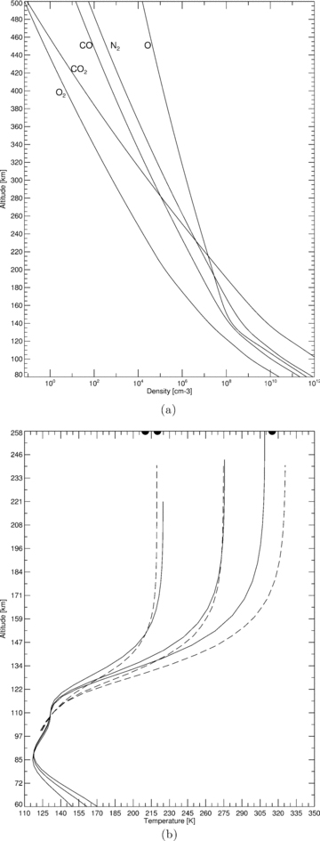
(a) Background neutral density profiles and (b) background neutral temperature as derived by MarTIM and used in the kinetic code. In part (b), left-to-right represent SMIN-to-SMAX for MarTIM (solid lines) and from MTGCM (see text) (dashed lines). Black dots represent spacecraft observations of exospheric temperatures for MGS and Mariner 6 & 7 (see text).

Open in new tabDownload slide

The model setup shown in Fig. 2(a) also gave us an O to CO₂ ratio of ≈1.7 per cent at 125 km and ≈2 per cent at 130 km. The O to CO₂ ratio at the altitude of the F1 ionospheric peak (≈130 km) is often quoted as a measure of the dissociation of the Martian atmosphere (Bougher et al. 2000) as the photochemically produced CO⁺₂ is quickly converted to O⁺₂ by reaction with O (Bougher et al. 1999). Occasionally, this ratio is also quoted at the altitude of the homopause (≈125 km) due to the important implications that O abundance has on the dominance of CO₂ cooling rates in the middle atmosphere. Typical values derived by other investigators range from 0.01 to 0.04 at 130 km over a range of solar activities and heliocentric distances (Bougher et al. 2000; Fox 2004). Values derived from MarTIM simulations for solar minimum, medium and maximum conditions (not shown) remain within this cited range.

2.3 Coupling the models

Coupling of the two models into Trans-TIM is achieved through interpolation of MarTIM's neutral background atmosphere (in fixed pressure vertical coordinates as noted already) on to the independent fixed altitude grid of the kinetic model. Number densities for neutral species CO₂, N₂, CO, O and O₂ are required by the kinetic code for the calculation of the column density of the one-dimensional atmospheric column through which the primary electron and solar fluxes are attenuated. These are interpolated from MarTIM's grid on to the Trans-TIM grid with a logarithmic interpolation routine. Neutral atmosphere temperatures from MarTIM are also taken and used by the kinetic code for the column density calculation. Finally, MarTIM's geopotential heights are required in order to determine the fixed altitude against which the neutral densities and temperatures are defined.

Since the coupled Trans-TIM model describes the ionosphere using a fixed altitude grid ranging from 80 to 500 km, the use of MarTIM's background atmosphere demands that we provide a neutral atmosphere from MarTIM's upper boundary (∼ 200–350 km) to the upper boundary of the kinetic model (500 km). Such an extrapolation was achieved by assuming this upper atmosphere region could be described by a hydrostatic distribution with isothermal structure and starting from the number densities given by MarTIM's upper boundary. Although the altitude region above MarTIM's upper boundary (∼ 200–350 km) is probably not in hydrostatic equilibrium in the actual Martian atmosphere the assumption should be sufficient in the region of the ionospheric peak, which is where our study is mostly concerned.

The solar EUV/XUV flux (λ≤ 105 nm) has been changed for this study to the solar flux model ‘SOLAR2000 Research Grade v2.28’ (see e.g. Tobiska et al. 2004), with empirical solar irradiances provided by Space Environment technologies. SOLAR2000 uses 39 energy bins ranging from 2.95 to 105.00 nm (∼420.3 to ∼11.8 eV). Considering this energy range for the production of primary (photo) electrons is justified since it allows us to consider photoproduction ranging from the various species ionization potentials (Fox et al. 2008) right the way through EUV to XUV irradiances.

Taking SOLAR2000 as a solar flux model at a heliocentric distance of 1 au, we account for the greater Mars-to-Sun distance by multiplying the fluxes in all 39 energy bins by the inverse square of the heliocentric distance. We also multiply the F_10.7 flux, which is simply an output of SOLAR2000 often used as a reference measure of solar activity, by the same factor and quote this new value throughout the present study. In this way, we can study different solar cycle conditions, although we note that the actual numerical value of the F_10.7 flux has no computational role in the calculations, it is simply quoted throughout this paper as a standard measure of solar activity.

The photoionization and electron collision cross-sections are the same as those used in a previous Mars atmosphere study using the kinetic model (Simon et al. 2008) namely from Torr & Torr (1985) for N₂, O₂, O, Hitchcock et al. (1980) and Avakyan (1998) for CO₂ and Tian & Vidal (1998) and Lummerzheim & Lilensten (1994) for the secondary ion productions

2.4 The problem to solve

As was discussed in Section 2.1, the computation of ion and electron densities by primary photoproduction (equation 3) is straightforward. However, using the primary electrons calculated to complete the full transport equation calculation for the secondary production by energetic electron propagation through the background neutral atmosphere (as it is described above) is a far more involved and complex computation. Thus, in the following section, we will describe the results of the full Trans-TIM calculation for primary and secondary ion and electron production using the kinetic code with MarTIM providing the neutral background atmosphere.

The main aim is to provide a method by which the secondary ion and electron production can be calculated rapidly using the production efficiency ε (defined as the ratio between the secondary and primary productions) as an intermediary. We will then use different neutral background atmospheres (as calculated by MarTIM) to show that while the production efficiency does vary with solar zenith angle it can be parametrized with a simple function. We also show that variations with solar cycle and solar longitude are negligible about the region of the primary and secondary production peaks.

Our study only considers solar zenith angles up to 90° since beyond this point the illumination rapidly fades as the Sun drops below the horizon. As a consequence, we calculate the primary photoproduction and secondary electron impact production peaks to rapidly decrease in magnitude to below the minimum value that we considered relevant for consideration (1 × 10⁻³ cm⁻³ s⁻¹). In turn, we found that under these swiftly changing conditions the production efficiency did not lend itself to any straightforward parametrization. The approach of this phenomena is discussed further below.

3 RESULTS

3.1 Polynomial fit to the production efficiency

Following a similar method of Lilensten et al. (2005), where the production efficiency for Titan's ionosphere was studied, we also fit the model efficiency profiles ε(z, χ) with a simple polynomial law. Initially, the production efficiency is defined as a function of altitude z and solar zenith angle χ. Of course given the dependence the ionosphere has on the background neutral atmosphere, one would also expect efficiency to be a function of solar cycle and Martian season. To start with, then we conducted model runs for a solar zenith angle of χ= 0° at solar longitude Ls= 180° (equinox) for solar minimum conditions (F_10.7,Mars= 31.3) and then later on studied the effect on the efficiency of varying the three variables solar zenith angle, solar longitude and solar cycle, preferably in an effort to reduce ε to a single dependency on altitude z.

Above a given transition altitude, we use a logarithmic fit in order to avoid oscillations in the fit due to high-order polynomials,

11

while below this transition altitude use a direct polynomial fit,

12

where z is the altitude in kilometres. The transition altitudes as well as the a_i and b_i coefficients for the 11 ion species CO⁺₂, CO⁺⁺₂, CO⁺, C⁺, N⁺₂, N⁺⁺₂, N⁺, O⁺₂, O⁺⁺₂, O⁺ and O⁺⁺ studied in this work, and for the electrons, are given in Table A1–A6 in Appendix A.

Our confidence in the physical consistency of the kinetic model and its calculation of the primary and secondary production rates and thus the efficiency meant that looking for a fit that had some basis in physics was not necessary (Lilensten et al. 2005). Therefore, our method for determining where the transition altitude should lie and what the most appropriate number (N or M) of coefficients to use in a particular species fit was to consider each species individually and to ensure minimum error between the kinetic model calculated vertical profile of efficiency and the polynomial fitted profile. As noted, the use of a logarithmic fit at high altitude ensured oscillations due to high-order polynomials were minimized and thus aided this process.

3.2 Production efficiency general trends

The Trans-TIM calculated ion production rates (cm⁻³ s⁻¹) for the 11 ion species studied in this report (and for the electrons) are shown in Fig. 3(a) for N⁺₂, N⁺, N⁺⁺₂ and the electrons, Fig. 4(a) for CO⁺⁺₂, CO⁺, C⁺ and O⁺ and finally Fig. 5(a) for O⁺₂, O⁺⁺₂, O⁺⁺ and CO⁺₂. In each case, the contribution from photo (primary) ionization, electron impact (secondary) ionization is plotted as well as their total contribution (i.e. the sum of primary and secondary). Then in each case, part (b) of the mentioned figures shows the production efficiencies (ε) that is secondary production divided by primary production calculated both by Trans-TIM and by the polynomial fit as described above.

Figure 3

(a) Total production (solid lines), primary (photo) production (dashed lines) and secondary production (dot–dashed lines) and (b) production efficiency [kinetic model result (crosses), polynomial fit (solid line) and transition altitude (dashed line)] versus altitude (km). Production rates are in units of cm⁻³ s⁻¹ versus altitude in km. Top left N⁺, top right N⁺⁺₂, bottom left electrons, bottom right N⁺₂.

Open in new tabDownload slide

Figure 4

(a) Total production (solid lines), primary (photo) production (dashed lines) and secondary production (dot–dashed lines) and (b) production efficiency [kinetic model result (crosses), polynomial fit (solid line) and transition altitude (dashed line)] versus altitude (km). Production rates are in units of cm⁻³ s⁻¹ versus altitude in km. Top left C⁺, top right O⁺, bottom left CO⁺⁺₂, bottom right CO⁺.

Open in new tabDownload slide

Figure 5

(a) Total production (solid lines), primary (photo) production (dashed lines) and secondary production (dot–dashed lines) and (b) production efficiency [kinetic model result (crosses), polynomial fit (solid line) and transition altitude (dashed line)] versus altitude (km). Production rates are in units of cm⁻³ s⁻¹ versus altitude in km. Top left O⁺⁺, top right CO⁺₂, bottom left O⁺₂, bottom right O⁺⁺₂.

Open in new tabDownload slide

The structure observed in the efficiency profiles of Figs 3(b), 4(b) and 5(b) deserves further explanation. The shape of the efficiency profiles comes about, in the main, simply due to the numerical effect of dividing the secondary production rate by the primary production rate. So the actual numerical value of the efficiency gives no indication that either primary or secondary production is particularly important at that location. It instead simply refers to their relative importance with respect to one another. Thus, an extremely large efficiency can occur when one divides a secondary production rate by a primary production rate that is far smaller in magnitude. But it may well be that both primary and secondary productions are negligibly small because all the efficiency describes are their magnitudes relative to one another. Indeed, as noted briefly already, in all the cases, we took the decision to set the efficiency to zero when the secondary production dropped below 1 × 10⁻³ cm⁻³ s⁻¹, showing no regard to whether an immense (or otherwise) primary production rate was in affect because clearly it was not creating a secondary production rate of any notable value.

Physically, the only parameters that are specific to each specie that could be responsible for the efficiency profile structure plotted are the photoabsorption and electron-impact cross-sections. After all, at any particular altitude, each specie exists under the same column of atmosphere (i.e. the same column depth) through which the same two sources of energy must pass (the photon and suprathermal electron fluxes). So each specie presents at a particular altitude will interact with the same intensity of primary energy source (from one specie to the next) and with the same intensity of secondary energy source (again from one specie to the next). Hence, at a particular altitude, it is the relationship, expressed in terms of the model energy grid, between the primary and secondary energy sources and the respective cross-sections of the atmospheric species present that will drive different production rate responses for each specie. It is the energy spectrum of the photon flux and its match with the photoabsorption cross-sections (in the case of the former), and the suprathermal electron intensity and its match with the electron-impact cross-sections (in the case of the latter) that will dictate which production type (primary or secondary) is dominant.

Bearing these statements in mind, we note two general trends in the efficiency profiles of fig. 3(b), 4(b) and 5(b) at low altitude. The first is where the efficiency continues to grow larger and larger as we decrease in altitude. So for example, the production efficiencies of N⁺⁺₂, CO⁺⁺₂ and O⁺₂ all begin to increase very quickly towards positive infinity as we approach the lower altitude boundary. The second trend is where the efficiency reaches a peak as we decrease in altitude before decreasing in the lowest altitude regions of the model. The production of N⁺ is an example of this trend, with the efficiency reaching a peak of ∼15 at ∼98.5 km before falling to ∼7 at ∼88 km.

The first trend is principally the numerical effect of dividing the secondary production rate by a primary production rate that is either far smaller or is decreasing more rapidly than the secondary production rate as we descend in altitude. It also indicates that at the lowest altitudes the photoabsorption cross-sections for species that exhibit this trend do not respond to the (probably high) photon energies present at these low altitudes and thus primary production remains low. Meanwhile there is a sufficient response by the electron impact cross-sections to the suprathermal electron energies present for secondary production to remain greater (relatively speaking) than primary production and thus cause the growth in efficiency observed. Remember here that since every altitude level is potentially a source of suprathermal electrons then transport effects can bring these electrons, with a greater range of energies, down to these low altitudes. That is to say, a greater range of suprathermal energies can be present relative to the range of photon energies present. This first trend is thus exhibited by species whose primary production is restricted in energy so they do not respond to the typical photon energies present at these altitudes.

For this first trend, we take the case of O⁺₂ as a good example of the numerical nature of this effect. From 100–83 km, the primary production rate drops almost 12 orders of magnitude where as the secondary production rate drops by just over 6 orders. Sure enough we see the efficiency climb from ∼16 to 1.22 × 10⁷ that is almost 6 orders of magnitude. But again this does not imply that some important effect is taking place, such as a production rate with an especially high magnitude or detailed structure. Indeed, the primary production rate is shown in Fig. 5(b) to be on the order of 5 × 10⁻² cm⁻³ s⁻¹ at 100 km (while the secondary rate is 8 × 10⁻¹ cm⁻³ s⁻¹) before the reductions just described have even begun. Thus, despite the efficiency profile growing rapidly below 100 km both, production rates are falling rapidly as we descend through the atmosphere. Finally, note that for O⁺₂ the secondary production rate dropped below 1 × 10⁻³ cm⁻³ s⁻¹ (and so was considered negligible) at and below 88.23 km.

The second trend in the efficiency profiles was noted above as the structure whereby the efficiency reaches a peak as we decrease in altitude before decreasing in the lowest altitude regions of the model. As noted, the production efficiency of N⁺ is a good example of this trend, with the efficiency reaching a peak of ∼15 at ∼98.5 km before falling to ∼7 at ∼88 km. This can essentially be understood as the converse of the first trend i.e. it is the result of a more rapid drop in the secondary production rate, below the efficiency peak, than there is in the primary production rate. The fact that there is a peak in the production efficiency in the first place is simply due to the growth in secondary production over and above primary production as the transport of suprathermal electrons down towards the peak gives greater opportunity for secondary production. This is to say that the range of suprathermal energies allows electron impact to dominate over photon production.

Typically, however, we find that in the lowest altitude regions the suprathermal electron flux (not shown) has a greater intensity in the lower model energies (say 0.1–4 eV) than it does in the upper energy regions, as secondary production can only produce electrons of lower energy and as collisions with the exponentially increasing neutral background atmosphere strips the flux of its energy. Therefore, this second trend is exhibited by species where the particular relationship between their primary and secondary productions favours the high-energy photons at the low altitudes rather than the low-energy suprathermal electrons. The neutral background swiftly removing higher energy suprathermals as we lead up to the peak while maintaining and harbouring a lower energy suprathermal presence that begins to dominate below the peak. Species electron impact cross-sections fail to respond to this change and secondary production drops more swiftly than primary production, hence the efficiency drops.

By and large the efficiency profiles at high altitude typically reach some constant value. This is simply because both the primary and secondary production rates remain parallel to one another throughout the upper regions of the model. Thus as primary production falls with increasing altitude and decreasing neutral number density so the secondary production follows suit due to both the reduced localized source function and the reduced likelihood of transport effects from higher altitudes. The only exception to this rule is specie C⁺ (Fig. 4) for whom secondary production dropped below 1 × 10⁻³ cm⁻³ s⁻¹ at and above 325 km before reaching any constant value. Secondary production for this specie continues to drop faster than primary production as we gain altitude hence the efficiency does also. We must come down in altitude, building up a sufficient component of transported suprathermals for secondary C⁺ production to become important, whereas for other species secondary production due to localized primary production is sufficient up through the highest altitudes to keep secondary and primary profiles almost parallel and thus efficiency constant.

3.3 The effect of variation in solar zenith angle on efficiency

To study the effect of the variation in solar zenith angle on the production efficiency, we used the three-dimensional neutral atmosphere provided by MarTIM. The results are shown in Fig. 6 for the CO⁺₂ production efficiency only. This variable was chosen for our representation of how efficiency responds to χ variation because of the dominance that neutral CO₂ has on the composition in the real and (MarTIM) modelled atmosphere, which would suggest that it plays an important role in the study of photon and suprathermal electron attenuation. Indeed, it was because of the importance of neutral species such as CO₂ that we ensured neutral diffusion processes were carefully modelled within MarTIM so that our description of the underlying physics was appropriate. Thus, we expect neutral CO₂ to be a sensitive indicator of any possible χ variation and in turn that CO⁺₂ ion production will reflect these changes.

Figure 6

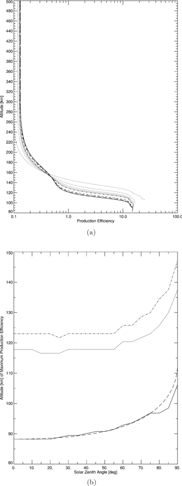
(a) CO⁺₂ production efficiency versus altitude (km) for solar zenith angle χ 0° (solid line), 25° (long-dashed line), 45° (short-dashed line), 70° (dot–dashed line). Then 75°, 80°, 85° and 90° are all shown with dotted lines. Their profiles can be identified in the lower altitude region up to 160 km by the increasing altitude of their peaks. (b) Altitude of maximum CO⁺₂ production efficiency versus χ (solid line), altitude of the maximum primary and secondary CO⁺₂ production (dot–dashed and dotted lines, respectively) and equation (13) (dashed line). Solar minimum (F_10.7,Mars= 31.3) and equinox (180°) throughout.

Open in new tabDownload slide

In Fig. 6(a), we present production efficiency altitude profiles for a spread of four solar zenith angles up to 70° (0°, 25°, 45° and 70°) and then a further four angles from 75° to 90°. Then in Fig. 6(b), we present profiles showing the variation in the altitude of the peak primary and secondary production (dot–dashed and dotted lines respectively) as well as a profile of the altitude of the peak efficiency as a function of solar zenith angle (solid line). From part (a) of this figure, you can see that the effect of an increasing solar zenith angle, up to ∼ 80° (the second dotted line), is essentially to move the lower region of the profile (around the primary and secondary production peaks) upwards. Then, in part (b) of this figure, you can see the extent of this altitude shift with solar zenith angle more clearly as the peak efficiency reaches ∼105 km at χ= 90° compared with ∼88 km at χ= 0°. Additionally, in part (b), we plot a function to describe numerically this increase in efficiency peak altitude (dashed line),

13

Where α= 15, β= 40 and γ= 25.

The derivation of this function follows the work of Lilensten et al. (2005) who fitted a similar function to the efficiency profiles from the Titan version of the Trans* kinetic model (with different coefficients of course). Thus, as was the case in Lilensten et al. (2005), there are two components of the χ angle influence on the production efficiency. The first [cos(χ)] reflects the close approximation, the modelled atmosphere makes, to an ideal Chapman atmosphere. Since CO₂ is the dominant species throughout a large part of the atmosphere (and certainly in the region of peak primary and secondary production), the altitude of the primary peak when acting under the local control of photochemical processes, depends upon how deeply into the atmosphere the solar radiation penetrates (as was discussed regarding the real Martian atmosphere in Section 1). Hence, the altitude of the primary production peak will follow a cos (χ) form. Then from the dotted line of Fig. 6(b) note that how the secondary peak altitude follows quite closely with the primary peak. This reflects the sufficient uniformity in atmospheric density as a function of solar zenith angle, a product once again of CO₂ dominance, in restricting transport effects (or at least restricting their variation with χ) and thus keeping the primary and secondary peaks almost parallel to one another. As the altitude of the primary peak rises, so does the secondary peak. In turn, the efficiency peak altitude will simply follow suit and maintain a similar dependence on the cos (χ) term.

The second component to the variation in efficiency versus χ angle comes from the behaviour of the [cos(χ)]^1/2 term, which Lilensten et al. (2005) cite as being due to transport effects. For lower solar zenith angles (we suggest up to 80°) transport effects in the region of the primary and secondary peaks are probably not dominant or are at least restricted, as we have just discussed, so that the [cos(χ)]^1/2 term will remain less important. It is only at higher χ angles where transport effects would become important, providing the linkage between a primary peak rising swiftly in altitude while the secondary peak remained at lower altitudes where the neutral density is greater. Since this occurs beyond χ= 90° and for secondary production rates that drop significantly below 1 × 10⁻³ cm⁻³ s⁻¹, we do not deal with these situations further.

For the behaviour in the high χ angle range from 75° to 90° that is approaching the limit of our function of equation (13) consider the set of dotted lines shown in Fig. 6(a), which represents this range in χ= 5° steps. Note that how the peak of the efficiency profile (and indeed the main body of the profile up to ∼160 km) begins to gain altitude far swifter than it did for the lower solar zenith angles. It is at these high χ angles that the efficiency profiles start to reflect the action of the Sun as it begins to set below the horizon of the tenuous Martian atmosphere. As this occurs, the whole primary (photo) production profile shifts upwards in altitude, chasing the remaining illumination. At the same time, its magnitude decreases as the background neutral atmosphere rapidly reduces in mass density at high altitude. Meanwhile the secondary production profile does not show nearly the same amount of vertical motion because electron impact still requires a dense neutral background atmosphere for sufficient ionization collisions to occur. The two processes are linked by transport effects bringing down suprathermal electrons from the high primary peak to the lower secondary peak.

Consequently, at any particular altitude the magnitude of secondary production will be far greater relative to the primary production since the two profiles now cover completely different altitude ranges for their completely different processes at these high solar zenith angles. Therefore, the magnitude of production efficiency (secondary production divided by primary production) will also swiftly increase as we move towards higher solar zenith angles and unfortunately its profile structure will begin to be poorly represented by equation (13). We suggest therefore that our polynomial fits in Appendix A and equations (11) and (12) and the fit with solar zenith angle (equation 13) are suitable only up to χ= 80°. Beyond this angle, we further note however that since the magnitude of the primary production rate is rapidly reducing as the profile climbs in altitude so too will the secondary production magnitude (and to below the rate 1 × 10⁻³ cm⁻³ s⁻¹ that we considered of notable magnitude). Therefore, we feel our work describes suitably the main bulk of the dayside ionosphere primary and secondary production.

3.4 The effect of variation of solar longitude on efficiency

One would expect that with the greater solar insolation at perihelion (∼40 per cent increase) that the atmosphere would expand and conversely as the Sun–Mars distance increased as we approach aphelion that the atmosphere would contract. Certainly, in the region of the thermosphere (150–280 km) where solar heating is most dominant, we can assume a variation in the distribution height of the neutral background atmosphere as the scaleheight tracks the changing temperatures: increasing with higher perihelion temperatures; decreasing at aphelion. Consequently, the number of atmospheric molecules and atoms in any vertical column [N_m(χ) =H_mn_m above the production peak altitude m] will also mimic this variation with solar insolation. But since the altitude of the peak (in an ideal Chapman atmosphere at least) will remain at wherever σN_m(χ) = 1 occurs then in turn we expect the altitude of the primary production profile will vary with the advancing Martian seasons.

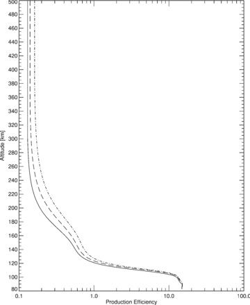
But of course it is a question of variation in the secondary production profile alongside the primary profile that will affect the production efficiency. If the variation in secondary production as solar longitude changes is different from the primary production variation then the efficiency will reflect this. We can see from Fig. 7 that indeed as solar longitude advances the efficiency does increase in the region of the thermosphere ∼150–280 km. Presumably this is as we shift from a localized to a more transport dominated secondary production rate. With a greater primary production at higher altitudes (with the expanded perihelion atmosphere), we have an increased component of transported primary electrons that contribute to secondary ionization. So the secondary production increases proportionately more than primary production due to this additional transported component and hence the efficiency increases. Of course, this variation in efficiency is restricted to the thermosphere ∼150–280 km where solar heating is dominant and even then to very limited extent.

Figure 7

CO⁺₂ production efficiency versus altitude (km) at solar zenith angle χ= 0° for solar longitude 0° (1.56 au equinox) (solid line), 90° (1.66 au northern summer solstice) (dashed line), 180° (1.47 au equinox) (dot-dashed line) and 270° (1.39 au southern summer solstice) (dotted line). Solar minimum (F_10.7,Mars= 31.3) throughout.

Open in new tabDownload slide

At lower altitudes, there is a very little variation in the production efficiency. This is a result of the dominance of CO₂ in the composition of the Martian atmosphere at these altitudes, which results in (a) reduced variation in solar flux intensity at these altitude levels and (b) similar variation in primary and secondary production despite the changing Martian season. This latter point is most likely due to the reduced role transport effects play in the lower atmosphere, regardless of the season, linking secondary production to localized primary production. This situation remains as solar longitude changes since the background lower atmosphere barely varies at all with solar longitude and thus production efficiency remains fairly stable. This situation will only become more apparent throughout the lower atmosphere as the dominance CO₂ continues to increase and the incident solar flux tails off completely. Thus, if one is only considering the altitude region of the CO⁺₂ production peak then one need not alter the polynomial fit coefficients from those provided as there is little variation to worry about despite the changing Martian season.

3.5 The effect of variation of the solar cycle on efficiency

In this final study of variation in production efficiency, we note from Fig. 8 that generally there are only slight changes in the production efficiency as the solar cycle advances. For reasons analogous to the above discussion about the variation in solar longitude, we find this to be most apparent in the lower altitude regions given the reduction in incident solar flux as one moves deeper into the atmosphere. Any change in solar flux due to the varying solar cycle will be minimal in these lower altitude regions thus the primary production will not change much. Since secondary production will remain linked to localized primary production this will not change much either. Hence, the production efficiency changes only slightly as the solar cycle advances.

Figure 8

CO⁺₂ production efficiency versus altitude (km) at solar zenith angle χ= 0° and solar longitude 180° for solar minimum (F_10.7,Mars= 31.3) (solid line), solar medium (F_10.7,Mars= 60.9) (dashed line) and solar maximum (F_10.7,Mars= 95) (dot–dashed line).

Open in new tabDownload slide

In the upper altitude regions of the thermosphere proper, one would not expect the height of the primary peak to vary with solar cycle in an ideal Chapman atmosphere (Ratcliffe 1972), it is independent of flux intensity. Although the primary production profile in the thermosphere above the peak will increase as the enhanced solar flux takes effect clearly there must be a relatively larger increase in secondary production since we can see in Fig. 8 that the efficiency is increasing with the solar flux. We would suggest that, just as in the case of advancing solar longitude, the effect of enhanced primary electron transport from the upper altitude regions will produce this additional secondary production and the increase in production efficiency seen. Of course, again just as with the seasonal variation, the effect is rather limited and we do not consider it necessary to adjust our parametrization to include this effect.

4 CONCLUSIONS

An analytic method has been discussed for the rapid computation of secondary ion and electron production due to electron impact of suprathermal electrons with the background neutral Martian atmosphere. Parameters were given (see the appendix) to allow the rapid computation of secondary ion production for 11 ion species (CO⁺₂, CO⁺⁺₂, CO⁺, C⁺, N⁺₂, N⁺⁺₂, N⁺, O⁺₂, O⁺⁺₂, O⁺, O⁺⁺) as well as for the secondary electron production. It was shown that while the efficiency (ε) of ion and electron production (ratio of secondary to primary production) does vary with solar zenith angle it could be parametrized with a simple function, given by equation (13). It was also shown that variations in the efficiency with solar cycle and solar longitude were negligible about the region of the primary and secondary production peaks, and thus that the parametrizations given did not need altering despite these varying conditions. Our future work will concentrate on including ionospheric chemistry in Trans-TIM and a better representation of magnetic fields in the code so that features such as the Martian magnetic anomalies can be studied.

WPN is supported by STFC and UCL. The authors would like to thank the referees for considering our paper and for their helpful requests and suggestions.

REFERENCES

Appendix

APPENDIX A: POLYNOMIAL COEFFICIENTS FOR USE IN EQUATIONS (11) AND (12)