


Abstract
In this paper we report the results of high-resolution circular spectropolarimetric monitoring of the Herbig Ae star V380 Ori, in which we discovered a magnetic field in 2005. A careful study of the intensity spectrum reveals the presence of a cool spectroscopic companion. By modelling the binary spectrum, we infer the effective temperature of both stars: 10 500 ± 500 K for the primary and 5500 ± 500 K for the secondary, and we argue that the high metallicity ([M/H]= 0.5), required to fit the lines, may imply that the primary is a chemically peculiar star. We observe that the radial velocity of the secondary's lines varies with time, while that of the primary does not. By fitting these variations, we derive the orbital parameters of the system. We find an orbital period of 104 ± 5 d and a mass ratio (MP/MS) larger than 2.9. The intensity spectrum is heavily contaminated with strong, broad and variable emission. A simple analysis of these lines reveals that a disc might surround the binary and that a wind occurs in the environment of the system. Finally, we performed a magnetic analysis using the least-squares deconvolved profiles of the Stokes V spectra of both stars and adopting the oblique rotator model. From rotational modulation of the primary's Stokes V signatures, we infer its rotation period P= 4.312 76 ± 0.000 42 d and find that it hosts a centred dipole magnetic field of polar strength 2.12 ± 0.15 kG, with a magnetic obliquity β= 66°± 5° and a rotation axis inclination i= 32°± 5°. However, no magnetic field is detected in the secondary, and if it hosts a dipolar magnetic field, its strength must be below about 500 G, to be consistent with our observations.
1 INTRODUCTION
Today, one of the greatest challenges in stellar physics is to understand the origin of the magnetic fields observed in stars across the Hertzsprung–Russell (HR) diagram. It is now well established that the magnetic fields of the Sun and other cool, low-mass stars are generated by a convective dynamo occurring in their external envelope. Their magnetic fields are of a complex structure, highly variable on short time-scales, and are strongly correlated with fundamental stellar parameters such as the rotation period, mass and age, consistent with the dynamo theory (Baliunas et al. 1995; Saar 1996; Donati et al. 2003, 2008).
Around 5 per cent of the main-sequence (MS), intermediate-mass A and B stars host organized magnetic fields, with strengths between 300 G and 30 kG, that are stable over tens of years (e.g. Aurière et al. 2007). These characteristics show no correlation with the mass, age or rotation period of the stars. These qualitative differences suggest a different origin of their magnetic fields. Some authors have proposed the generation of magnetic fields inside the convective core of the intermediate-mass stars, with a similar dynamo process as in the low-mass stars, that would diffuse through their radiative envelope to reach the surface. However, this mechanism is not able to reproduce the observed field characteristics nor can it explain the long-term stability of these magnetic fields (Moss 2001).
Currently, the favoured scenario for the origin of magnetic fields in A- and B-type stars is the so-called fossil field hypothesis. This model proposes that the magnetic fields observed in the intermediate-mass stars are relics, either of the Galactic magnetic field present in the molecular clouds from which the stars formed or generated by a dynamo during the first stages of stellar formation. Once a star is born, the relic magnetic field would necessarily survive the various stellar evolutionary stages from the pre-main-sequence (PMS) to the post-main-sequence phases, without significant regeneration.
Magnetic fields are observed among molecular clouds with magnetic strengths between 1 and 100 μG (Heiles 1997) and also among the MS A/B stars. Until recently, we were missing information about the magnetic properties of the PMS intermediate-mass stars. According to the fossil theory, 1–10 per cent of PMS intermediate-mass stars should be magnetic with similar magnetic topology than in the MS A/B stars and with magnetic strengths consistent with the conservation of the magnetic flux from the PMS to the MS stages.
The Herbig Ae/Be (HAeBe) stars have been defined by Herbig (1960) as emission line stars of spectral type A or B, associated with nebulae, and situated in an obscured region. These characteristics strongly suggest that the HAeBe stars are very young, still completing their PMS phase. We therefore consider that the HAeBe stars are the PMS progenitors of the MS A/B stars. Many authors have predicted the presence of magnetic fields in these stars (Catala et al. 1999; Hubrig, Schöller & Yudin 2004; Wade et al. 2007). Some of them try to detect them, without much success, except in HD 104237 (Donati et al. 1997).
In order to provide new observational constraints on the fossil field hypothesis and explore the magnetic properties of the PMS intermediate-mass stars, we performed a survey of ∼70 HAeBe stars with the new generation of high-resolution spectropolarimeters: ESPaDOnS, installed at the Canada–France–Hawaii Telescope (CFHT) in Hawaii, and Narval, installed at the Bernard Lyot Telescope (TBL) at Pic du Midi in France (Alecian et al. in preparation). Among this sample, we have discovered four new magnetic HAeBe stars, including V380 Ori (Wade et al. 2005; Catala et al. 2007; Alecian et al. 2008; Folsom et al. 2008). Our survey has thereby brought the first strong arguments in favour of the fossil theory. In particular, we have concluded that ∼6 per cent of the HAeBe stars observed in our survey are magnetic.
To go further, we have characterized the magnetic fields of three of these stars (HD 200775, Alecian et al. 2008; HD 190073, Catala et al. 2007; HD 72106, Folsom et al. 2008) in order to compare their magnetic topologies and strengths with those of the MS A/B stars. We have found that the magnetic HAeBe stars host large-scale organized magnetic fields, with important dipole components with polar strengths between 300 G and 1.4 kG, in agreement with those of the MS stars and with the fossil model.
V380 Ori, of spectral type B9, has been classified as an HAeBe star by Herbig (1960). This star is associated with many Herbig–Haro objects, with the H ii region NGC 1999 in the Orion OB1c association (Corcoran & Ray 1995), and its spectrum contains strong emission lines (Finkenzeller & Jankovics 1984; Finkenzeller & Mundt 1984). Hillenbrand et al. (1992) classify V380 Ori as a Group I object whose spectral energy distribution (SED) in the infrared (IR) is similar to those of the low-mass PMS T Tauri stars. The SED is well reproduced with a model of a flat, optically thick accretion disc. These results firmly establish the PMS status of V380 Ori.
V380 Ori was detected as a rather bright X-ray source by ROSAT (Zinnecker & Preibisch 1994). Subsequent X-ray grating spectroscopy with Chandra (Hamaguchi, Yamauchi & Koyama 2005) implied a single-temperature plasma with a relatively high temperature, leading these authors to speculate that magnetic activity was occurring in the close environment of the star. However, as pointed out by Stelzer et al. (2005), due to the small binary separation of V380 Ori (see Section 3.1), Chandra was not able to resolve the system and the origin of the (apparently single) X-ray source remains obscure.
The magnetic field of V380 Ori was detected during the first run of our Herbig survey, using ESPaDOnS at the CFHT (Wade et al. 2005). This paper reports subsequent observations of V380 Ori acquired between 2005 and 2007 as well as the analysis that we have performed in order to characterize its magnetic field. In Section 2, we describe the observations and data reduction. Section 3 describes the intensity spectrum and reports the discovery of a spectroscopic companion. In Section 4 we determine the fundamental properties of both components, and in Section 5 we describe the magnetic field analysis performed on both the primary and secondary stars. Finally, a discussion and a conclusion are given in Section 6.
2 OBSERVATIONS AND DATA REDUCTION
Our data were obtained using the high-resolution spectropolarimeters ESPaDOnS, installed on the 3.6 m CFHT, and Narval, installed on the 1.9 m TBL (Donati et al. in preparation) during many observing runs spread over nearly 3 years from 2005 February to 2007 November. We obtained 24 circular polarization (Stokes V) spectra covering the entire optical spectrum from 3690 to 10 480 Å, with a resolving power λ/Δλ= 65 000 and with a signal-to-noise ratio (S/N) between 70 and 290. Table 1 presents the log of the observations.
Log of the observations. Columns 1 and 2 give the UT date and the Heliocentric Julian Date of the observations. Column 3 gives the total exposure time. Column 4 gives the peak S/N (per ccd pixel, integrated along the direction perpendicular to the dispersion) in the spectra, at the wavelength indicated in Column 5. Columns 6 and 7 give the S/N in the reconstructed LSD Stokes V profiles of the primary (P) and the secondary (S), respectively. Column 8 gives the longitudinal magnetic field of the primary, Column 9 gives the rotation phase of the primary as derived in Section 5.2 and Columns 10 and 11 give the radial velocities of both components of the system. Column 12 gives the instrument used.
| Date UT time | HJD (2 450 000+) | texp (s) | S/N | λ (nm) | S/N (LSD) | Bℓ (G) | Rotation phase | vradP (km s−1) | vradS (km s−1) | Instrument | |
| P | S | ||||||||||
| (1) | (2) | (3) | (4) | (5) | (6) | (7) | (8) | (9) | (10) | (11) | (12) |
| 2005/02/20 9:32 | 3421.9000 | 4800 | 122 | 809 | 283 | 752 | −165 ± 190 | 0.58 | 28.2 ± 1.2 | 52.6 ± 5.6 | ESPaDOnS |
| 2005/08/26 14:18 | 3609.093 97 | 4800 | 286 | 809 | 948 | 2366 | −501 ± 62 | 0.99 | 28.1 ± 1.0 | 26.8 ± 5.2 | ESPaDOnS |
| 2006/01/09 11:32 | 3744.985 82 | 4000 | 189 | 809 | 564 | 1363 | 410 ± 103 | 0.50 | 27.8 ± 1.0 | 44.9 ± 3.9 | ESPaDOnS |
| 2006/01/12 12:45 | 3748.036 50 | 1600 | 121 | 809 | 362 | 765 | 174 ± 168 | 0.21 | 27.6 ± 1.2 | 42.5 ± 4.8 | ESPaDOnS |
| 2006/02/11 9:48 | 3777.911 78 | 3200 | 193 | 809 | 605 | 1516 | −347 ± 98 | 0.13 | 27.7 ± 1.2 | 15.5 ± 8.6 | ESPaDOnS |
| 2006/02/12 9:29 | 3778.898 36 | 3200 | 193 | 809 | 634 | 1561 | 209 ± 92 | 0.36 | 27.6 ± 1.1 | 15.9 ± 6.9 | ESPaDOnS |
| 2006/02/13 9:48 | 3779.911 16 | 3200 | 149 | 809 | 439 | 1111 | 186 ± 129 | 0.60 | 28.1 ± 1.1 | 15.5 ± 5.9 | ESPaDOnS |
| 2007/03/17 19:47 | 4177.324 49 | 6300 | 163 | 731 | 530 | 1336 | −89 ± 96 | 0.74 | 28.2 ± 1.1 | 28.6 ± 6.7 | Narval |
| 2007/11/06 2:44 | 4410.617 90 | 6300 | 120 | 731 | 381 | 942 | −282 ± 161 | 0.84 | 28.0 ± 2.0 | 12.8 ± 6.6 | Narval |
| 2007/11/06 4:45 | 4410.702 06 | 6800 | 161 | 731 | 529 | 1327 | −143 ± 114 | 0.86 | 28.2 ± 1.2 | Narval | |
| 2007/11/07 2:12 | 4411.595 68 | 6600 | 163 | 731 | 525 | 1323 | −400 ± 121 | 0.06 | 27.6 ± 1.3 | Narval | |
| 2007/11/07 4:56 | 4411.709 53 | 6800 | 138 | 731 | 433 | 1076 | −367 ± 140 | 0.09 | 27.6 ± 1.5 | 11.3 ± 7.4 | Narval |
| 2007/11/08 2:36 | 4412.612 33 | 6800 | 113 | 731 | 349 | 858 | −62 ± 172 | 0.30 | 27.4 ± 2.1 | 12.5 ± 15.0 | Narval |
| 2007/11/08 4:52 | 4412.707 34 | 7500 | 142 | 731 | 441 | 1116 | 84 ± 142 | 0.32 | 27.3 ± 1.5 | 12.3 ± 8.1 | Narval |
| 2007/11/09 2:59 | 4413.628 80 | 7600 | 71 | 731 | 207 | 508 | 723 ± 319 | 0.54 | 27.8 ± 3.0 | 9.9 ± 15.0 | Narval |
| 2007/11/09 5:06 | 4413.717 13 | 6600 | 98 | 731 | 276 | 698 | 698 ± 255 | 0.56 | 28.0 ± 1.8 | 11.1 ± 11.1 | Narval |
| 2007/11/10 2:52 | 4414.623 96 | 6800 | 178 | 731 | 559 | 1408 | 19 ± 106 | 0.77 | 28.1 ± 1.2 | 11.5 ± 6.4 | Narval |
| 2007/11/10 4:51 | 4414.706 30 | 6800 | 156 | 731 | 489 | 1242 | −189 ± 128 | 0.79 | 28.2 ± 1.3 | 11.7 ± 7.2 | Narval |
| 2007/11/11 3:06 | 4415.633 37 | 6920 | 188 | 731 | 607 | 1513 | −336 ± 102 | 0.00 | 27.6 ± 1.1 | 11.1 ± 5.9 | Narval |
| 2007/11/11 5:06 | 4415.717 11 | 6920 | 192 | 731 | 616 | 1555 | −619 ± 106 | 0.02 | 27.6 ± 1.2 | Narval | |
| 2007/11/12 3:21 | 4416.643 86 | 6280 | 184 | 731 | 613 | 1533 | −108 ± 107 | 0.24 | 27.1 ± 1.2 | Narval | |
| 2007/11/12 5:11 | 4416.720 18 | 6280 | 194 | 731 | 605 | 1527 | −16 ± 109 | 0.25 | 27.2 ± 1.2 | 9.7 ± 5.8 | Narval |
| 2007/11/13 3:15 | 4417.639 78 | 6800 | 199 | 731 | 656 | 1645 | 395 ± 94 | 0.47 | 27.6 ± 1.1 | 11.7 ± 5.6 | Narval |
| 2007/11/13 5:13 | 4417.722 10 | 6800 | 192 | 731 | 608 | 1540 | 510 ± 111 | 0.49 | 27.7 ± 1.2 | 11.0 ± 5.2 | Narval |
We used both instruments in the polarimetric mode. Each Stokes V observation was divided into four sub-exposures of equal time in order to compute the optimal extraction of the polarization spectra (Donati et al. 1997; Donati et al., in preparation). We recorded only circular polarization, as the Zeeman signature expected in linear polarization is about one order of magnitude weaker than circular polarization. The data were reduced using the ‘libre esprit’ package especially developed for ESPaDOnS and Narval, and installed at the CFHT and at the TBL (Donati et al. 1997; Donati et al., in preparation). After reduction, we obtained the intensity Stokes I and the circular polarization Stokes V spectra of the star observed, both normalized to the continuum of V380 Ori. A null spectrum (N) is also computed in order to diagnose spurious polarization signatures and to provide an additional verification that the signatures in the Stokes V spectrum are indeed real (Donati et al. 1997).
3 PROPERTIES OF THE INTENSITY SPECTRUM
3.1 V380 Ori: an SB2 system
Many authors have mentioned the presence of a companion around the variable primary star of V380 Ori. Jonckheere (1917) was the first to observe a companion of visual magnitude equal to 13 mag at a distance of 3 arcsec and a position angle of 220°. However these observations were not confirmed by Herbig (1960), who proposed that Jonckhere was observing bright nebulosities in the vicinity of the central star.
Later, Leinert et al. (1994) and Leinert, Richichi & Haas (1997) detected an IR companion using speckle interferometry, a detection that was confirmed by Smith et al. (2005) and Baines et al. (2006) using the same technique. The angular separation between the primary and the IR companion is 0.154 arcsec, that is 62 au at a distance of 400 pc (Leinert et al. 1997). Bailey (1998) obtained spectroscopic observations of a sample of PMS stars, including V380 Ori, 2 years after the observations of Leinert (1994, 1997), and detected a companion using the spectro-astrometry technique. They measured a position angle of 207°, which is very close to the measurement of Leinert et al. (1997), and they suggested that the fainter component of the system has the greater equivalent width of Hα. Bouvier & Corporon (2001) analysed the system using high-angular resolution spectro-imaging. They detected the companion in 1993 December in only the three reddest photometric bands J, H and K. They derived a separation between the primary and the secondary of 0.14 arcsec and a position angle of 205°. All of these results are generally consistent with the presence of an IR-bright but optically faint companion star separated from the B9 primary by ∼0.15 arcsec.
Corcoran (1994) detected the Li i 6707 Å line in the spectrum of V380 Ori, confirmed later by Corporon & Lagrange (1999) and Blondel & Tjin A Djie (2006). Corporon & Lagrange (1999) attributed the Li line to a companion of spectral type later than F5, but they did not detect any radial velocity variations in the spectral lines of the primary.
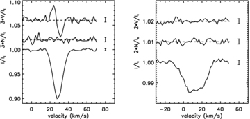
In our spectra, we confirm the detection of the Li i 6707 Å line and detect the presence of other lines belonging to a cool companion (Fig. 1). We observe that the radial velocity of the lines of the cool companion (hereinafter the ‘secondary’), including the Li i line, vary with a time-scale of a month, while the radial velocity of lines of the B9 HAeBe star (the ‘primary’) does not vary detectably with time (see Fig. 1). The study of the radial velocities presented in Section 4 leads to an estimate of the upper limit of the separation between both stars: a sin i < 0.33 au, which is around 200 times smaller than the separation observed between the IR companion and the primary star by Leinert et al. (1997). For these reasons, we conclude that the spectroscopic companion cannot be the IR-bright companion observed using speckle interferometry and that V380 Ori is therefore a triple system. In the following the primary (V380 Ori A – the B9 HAeBe star) and the secondary (V380 Ori B – the cooler companion) stars refer to the spectroscopic components, the primary being the hottest and most luminous. The tertiary refers to the IR-bright companion. The large luminosity ratio of the spectroscopic components, their small angular separation (a sin i < 0.83 mas, assuming a distance of 400 pc) and the relatively faint visual magnitude (V= 10.2) of the system explain why the secondary has never been directly detected in the past.
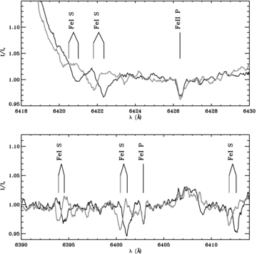
Selected regions of the spectrum of V380 Ori observed on 2006 January 9 (black line) and 2006 February 11 (grey line) around 6425 Å (top) and around 6400 Å (bottom). The positions and ions of the lines are indicated with a vertical black line for the January spectrum and with a vertical grey line for the February spectrum. The labels P and S beside the ion identification indicate the primary and secondary, respectively. Note the radial velocity variation of the lines of the secondary component, while no shift is observed in the radial velocity of the primary's lines.
3.2 Fitting of the intensity spectrum
In order to determine the effective temperatures of both stars and their luminosity ratio, we have fitted the intensity spectrum of V380 Ori with a synthetic spectrum calculated as follows. We used the code binmag1 developed by Oleg Kochukhov to calculate the composite spectrum of the binary star. This code takes as input two synthetic spectra of different effective temperatures and gravities, each corresponding to one of the two components. The code convolves the synthetic spectra with instrumental, turbulent and rotational broadening profiles and combines them according to the radii ratio of the components specified by the user, and the flux ratio at the considered wavelength given by the atmosphere models, to produce the spectrum of the binary star. The individual synthetic spectra were calculated in the local thermodynamic equilibrium (LTE) approximation, using the code synth of Piskunov (1992). synth requires, as input, atmosphere models, obtained using the atlas 9 code (Kurucz 1993) and a list of spectral line data obtained from the vald data base1 (Vienna Atomic Line Data base).
We compared the observed spectrum of V380 Ori to synthetic binary spectra using effective temperatures ranging from 9500 to 11 500 K for the primary and from 4500 to 6500 K for the secondary, and varying the ratio of radii from 1.0 to 1.8. In order to determine the temperature of the primary, we first focused on regions of the spectrum containing no significant circumstellar emission and lines from the primary not blended with the secondary. Then we varied the temperature of the secondary in order to reproduce all identified lines of the secondary. We find that the observed spectrum is well fitted with effective temperatures of 10 500 ± 500 K and 5500 ± 500 K for the primary and the secondary, respectively, and with a ratio of radii equal to 1.5 ± 0.2, where the uncertainties are at the 2σ confidence level. For both components we used a surface gravity (g) given (in cgs units) by log g= 4.0, consistent with the evolutionary stage of these stars. The strong emission contamination does not allow us to measure this characteristic directly. Our spectroscopic determination of the temperature of the primary is consistent with previous determinations of its spectral type, found to be between B9 and A1 (Herbig & Kameswara Rao 1972; Finkenzeller & Mundt 1984; Hillenbrand et al. 1992).
We also find that the portion of the spectrum not contaminated with emission requires a higher metallicity than the Sun in order to adequately fit the lines of the primary. The best-fitting metallicity is [M/H]= 0.5. In Fig. 2, the upper panel shows the observed spectrum superimposed with a synthetic spectrum calculated using binmag1 and a solar metallicity, while in the lower panel the synthetic spectrum has been calculated using a metallicity of [M/H]= 0.5. It is however less evident that the secondary requires a high metallicity in order to fit its lines. While a higher metallicity seems to provide a marginally better fit to the unblended lines of the secondary, the differences between the solar metallicity and the [M/H]= 0.5 spectra are not sufficiently small as to be insignificant in comparison with the uncertainties of the observed spectrum.
![Portion of the spectrum observed on 2005 August 26 (black full line) superimposed with the synthetic spectrum of the binary (red dashed line) calculated with a solar metallicity (upper) and a metallicity of [M/H]= 0.5 (lower). The positions and the ions of the lines are indicated with vertical lines. The labels P and S beside the ion identification indicate lines of the primary and secondary, respectively.](https://oup.silverchair-cdn.com/oup/backfile/Content_public/Journal/mnras/400/1/10.1111_j.1365-2966.2009.15460.x/1/m_mnras0400-0354-f2.jpeg?Expires=1749869389&Signature=v7Xli6menXWlHfbsDaaMw9uj6oYeJRQZFcX-wQ76xW43VEWgpw3ceb-l16yp7GVZGgwwY3ktmkcDFGeRylj39mt5iPz6TXyFI-bnFL2jbcAGZr5qWil4A0Y5XmpG4IQ7r5OrYqmddBz0vnmJjrohMUiao-9Ez9kTcVTg4sgwreFNyOa8s1bRL7A6FSpnogqeFxlONVeS3JWmqaL9LuSA0Bzth4R8dAi1Vpbp~ylPptJNFuj5nBKfKeNTRdqQUlix5nXX8-llsMXIyYn3GEdF-fLr0RhLMJCskcPMb7JiG55odlfgk90Z8Xcn4uMO433C96egybiAc0W2mlWEMVHpyQ__&Key-Pair-Id=APKAIE5G5CRDK6RD3PGA)
Portion of the spectrum observed on 2005 August 26 (black full line) superimposed with the synthetic spectrum of the binary (red dashed line) calculated with a solar metallicity (upper) and a metallicity of [M/H]= 0.5 (lower). The positions and the ions of the lines are indicated with vertical lines. The labels P and S beside the ion identification indicate lines of the primary and secondary, respectively.
We can wonder if the high metallicity found in the primary reflects inaccurately determined parameters of the binary system. Using the ratio of radii to the temperatures of both components, we find that the derived luminosity ratio is equal to rL=LP/LS= 30+37−17, which implies that the luminosity of the system is dominated by the luminosity of the primary. Therefore, increasing RP/RS cannot result in a significant increase in the depth of the synthetic lines of the primary to provide a better fit to the observed lines. Furthermore, we cannot sufficiently strengthen the computed lines of Fe, Ti and Si of the primary by changing the effective temperature or surface gravity within reasonable ranges. We therefore confidently conclude that the metallicity of V380 Ori A is higher than in the Sun.
It is well known that some magnetic intermediate-mass stars on the MS show chemical peculiarities characterized by overabundances of elements such as iron, silicon and titanium. These stars are called the magnetic chemically peculiar Ap/Bp stars. First, as the primary of V380 Ori is magnetic, it is reasonable to consider that it might be a chemically peculiar star or that it may evolve to become one. Secondly, the spectrum of V380 Ori A is dominated with iron, titanium and silicon lines, and the measurement of the metallicity described above has been mainly performed using these lines. The high metallicity that we measure may therefore reflect only overabundances in iron, titanium and silicon. Thirdly, it seems that the diffusion processes occurring at the surfaces of chemically peculiar stars are sufficiently rapid to observe peculiar stars at the PMS stage of stellar evolution (Vink, Michaud and Alecian, private communication). However, at this stage the stars, still surrounded by gas and dust, might experience exchanges of matter with their surroundings, by accretion and winds, which could result in instabilities and in mixing of the stellar atmosphere. The diffusion processes are therefore unlikely to be efficient during the PMS phase. Indeed, we do not observe any chemical peculiarities at the surface of either of the young magnetic HAeBe stars HD 200775 and HD 190073 (Catala et al. 2007; Alecian et al. 2008), whereas they are observed in the more evolved star HD 72106 (Folsom et al. 2008). The strong emission and variability observed in the spectrum of V380 Ori suggest that its environment is highly dynamic, with plenty of gas and dust. However, it is not clear if exchanges of matter occur between the star and its environment. Furthermore the strong magnetic field that we observe at the stellar surface could sufficiently stabilize and isolate its atmosphere, to allow gravitational settling and radiative diffusion to occur. Therefore, we tentatively conclude that the V380 Ori SB2 system is composed of a chemically peculiar primary star and a secondary of solar metallicity. More observations of a better S/N, as well as a thorough study of the detailed chemical abundances of both components, are required to confirm this proposal.
3.3 The emission lines
3.3.1 Description
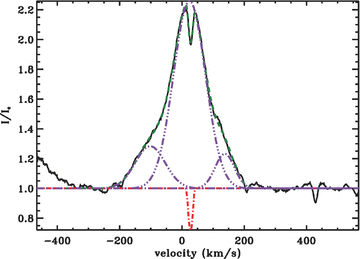
The most evident characteristic of the Stokes I spectrum of V380 Ori is a strong contamination by circumstellar emission. All Balmer and Paschen lines visible in the spectrum (from Hα to Hε and from P11 to P20) as well as the Ca ii 8498 Å and 8662 Å lines are filled with emission. Hα, Hβ, the Paschen lines and the IR Ca ii lines exhibit a single-peaked emission profile. Hα shows a faint blueshifted P Cygni absorption component that may originate from a wind (see Figs 3a and c for Hα). The radial velocity of the P Cygni component changes with time, from −350 km s−1 to −250 km s−1, with time-scales of the order of a few days. Our data reveal no periodicity of these variations. In Fig. 3(b) are plotted the differences between the Hα profiles and the mean of these profiles, revealing changes in the shape and amplitude of the Hα profile on time-scales of the order of days and sometimes hours (e.g. between both Hα profiles obtained on 2007 November 9 taken 2 h apart). Complex structures seem to appear and disappear through the Hα profile on time-scales of a day. The same kind of structures appear in the Hβ profiles, in the same wing (either blue or red) as the Hα profile, but at different radial velocities.
(a) Hα profiles of the 24 observed spectra of V380 Ori. The date is indicated on the left side of the profiles. Note the temporal variations of the amplitude, as well as the appearance and disappearance of substructures in the red and blue wings of the profile. (b) Difference between the Hα profiles and the mean Hα profile. (c) Same as (a) but plotted on a different scale to better show the absorption features in the blue wing of the profile.
Most of the metallic photospheric lines in the spectrum of V380 Ori are also superimposed with emission. The emission is correlated with the intrinsic central depth and the excitation potential of the lines: at constant excitation potential, the greater the central depth, the greater the emission, while at constant central depth, the greater the excitation potential, the lower the emission. Catala et al. (2007) observe in the spectrum of another magnetic HAe star HD 190073 a similar correlation: the emission increases with the central depth of the lines. By re-analysing the spectrum of this star, we also find the following at constant central depth: the greater the excitation potential, the lower the emission. These behaviours have also been observed in numerous non-magnetic HAeBe stars (Alecian et al. in preparation). The origin of these correlations is still not understood.
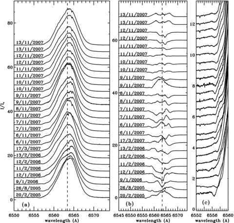
Most Fe ii and Ti ii lines in the spectrum show strong emission with a presumably photospheric component in absorption, as illustrated in Fig. 4. The amplitude and the shape of these emission lines changes on a time-scale of days and sometimes of hours. While the profiles of most of the lines are well reproduced with a simple Gaussian, the strongest emission lines require a slightly more complex model. These emission lines can be described as the superposition of three different Gaussian emissions: a strong main emission component superimposed with two smaller emissions, one in each wing of the main component. We have fitted the strongest unblended emission lines using the following model. Each of the three emission components is fitted using a simple Gaussian with three free parameters: the amplitude, the full width at half-maximum (FWHM) and the centroid. When necessary, we also fitted the photospheric absorption using the convolution of a rotation profile (itself a function of v sin i and vrad) with a Gaussian of instrumental width (Gray 1992). This convolution is then multiplied by a scale factor in order to fit the depth of the absorption component. An example of the results of this fitting procedure is shown in Fig. 5. While the FWHMs of the two wing Gaussians vary from one observation to another, and from one line to another, the strongest emission retains the same value of FWHM, around 65 km s−1. Temporal variations of the amplitude of the emission, and of the two wing emissions, are observed, but no periodicity is detected. The origin of these emissions is not known. The symmetry of the centroids of the wing emission with respect to the radial velocity of the primary suggests that they may arise from a disc surrounding the central star. However the temporal variations of these emissions, that is variations of their amplitude, centroid and FWHM, are difficult to explain in this context. While the main emission component of the iron and titanium lines is, most of the time, redshifted compared to the radial velocity of the primary star, we observe, in the same spectrum, a few lines for which the main emission component is centred or blueshifted compared to the radial velocity of the star. This behaviour is variable with time, and is not yet understood. Finally, in the few cases in which we include the photospheric component into the fit, the radial velocities and the v sin i of this component are consistent with the values for the primary's photospheric lines found in Section 4.2, by fitting the Stokes I least-squares deconvolved (LSD) profiles.
Portion of the spectrum observed on 2005 August 26 (black full line) and on 2006 February 12 (green dashed line). The positions and the ions of the lines are indicated with vertical lines. The label P beside the ion identification indicates lines arising from the primary. Note the variation in the emission of the metallic lines of the primary.
Fe ii 4351 Å lines in the spectrum of V380 Ori observed on 2005 August 26 (black full line) superimposed with the fit (green dashed line). The four components of the fit, described in Section 3.3.1, are also plotted: the three Gaussian functions modelling the emission in blue dot–dot–dot–dashed lines and the photospheric absorption in the red dot–dashed line.
All the emission lines (except Hα, Hβ, the Paschen lines and the IR Ca ii lines) show a photospheric component, as already observed in the spectrum of HD 190073. Furthermore, the characteristic of the main emission component is similar to the emission lines of HD 190073: in both cases the FWHM is around 65 km s−1, constant along the time and through the spectrum. As in Catala et al. (2007), we do not find a suitable scenario to explain these characteristics. These similarities cannot be due to a coincidence and these emission properties therefore bring strong constraints on the forming region.
Both Ca ii H and K lines show clear P Cygni profiles, as already observed by Herbig (1960) and Finkenzeller & Mundt (1984). The shape of the emission profile is also composed of a main emission component with wing components similar to those of the Fe ii and Ti ii lines. The radial velocity of the blue absorption part of the P Cygni profiles also varies with time from −190 to −160 km s−1 with respect to the rest wavelength of the Ca ii lines.
The He i 5876 Å and He i 6678 Å lines show broad emission superimposed with a strong absorption component. Using a Gaussian function, we have fitted only the emission component of these lines. We find that the equivalent width of the emission varies from 9 to 27Å for He i 5876 Å and from 10 to 18 Å for He i 6678 Å, while their FWHMs vary from 130 to 200 km s−1 and from 130 to 180 km s−1, respectively. Their centroids vary from −30 to 30 km s−1 and are, most of the time, blueshifted with respect to the radial velocity of the primary. Interestingly, no emission, and only a small absorption feature, is visible at 5876 Å in the spectrum obtained by Finkenzeller & Mundt (1984).
The O i 7773 Å triplet is in emission, and superimposed with the photospheric absorptions. Its equivalent width varies with time from 3 to 7 Å, with temporal variations similar to the He i and Balmer lines, but still without any periodicity.
3.3.2 Origin of the emission
The angular separations between the primary and the two companions (0.83 and 154 mas for the secondary and tertiary, respectively) are smaller than the pinhole aperture of the ESPaDOnS instrument (1.6 arcsec). Therefore, all optical contributions from the three components are present in the spectra that we obtained. While no photospheric lines from the tertiary are detected in our spectra, we can wonder if a contribution from this component exists in the emission lines. Leinert et al. (1997), using speckle interferometry, measured the flux of the primary and the tertiary separately in six IR photometric bands (I′, J, H, K, L′ and M). They fitted the SED using two models: model (a) is composed of a system in which the primary dominates the tertiary at all wavelengths whereas model (b) assumes an optical primary and an IR companion. In both cases, the primary is dominant at optical wavelengths. It is therefore unlikely that the tertiary contributes to the emission in the optical spectrum of the system.
Excluding the Balmer lines, the major emission in the spectrum is observed only in the lines of the primary – such emission is a common characteristic of HAeBe stars. Our modelling of a few emission lines shows that the wing emission components are symmetric with respect to the radial velocity of the primary. Although the main emission component is not perfectly centred on the radial velocity of the primary, this characteristic is commonly observed in other HAeBe stars. Furthermore, the lines of the secondary that are not blended with lines from the primary show emission that is much weaker than that observed in the primary's lines. Finally, the variability observed in the strong emission lines described above has been compared to the radial velocity variations of the secondary, and no correlation has been observed. The emissions observed in the metallic lines of the primary are therefore likely originating from the primary star of the system. However, the small separation (a sin i < 0.33 au) between the spectroscopic component and the fact that the typical length of the discs surrounding HAeBe stars is larger than few au (Hillenbrand et al. 1992) leads to the conclusion that the disc would be circumbinary, instead of circumstellar.
We cannot firmly conclude that this is true for the Balmer lines, and especially Hα and Hβ. The structure and the variability observed in these lines are complex and our observations cannot rule out the fact that the secondary might contribute to them and even the tertiary as suggested by the spectro-astrometry study of Bailey (1998).
The temporal variations observed among the emission features of the spectrum of V380 Ori are certainly the result of strong and rapid dynamic phenomena in the circumstellar environment of the star, which would be the subject of a very interesting study, but which is not the purpose of this paper. We therefore do not go further in the description and analysis of the emission features observed in the spectrum. Instead, we will look more closely at these characteristics in a future paper that will involve not only high S/N spectroscopic observations, but also other types of observations such as linear polarimetry and interferometry, as well as sophisticated models capable of reproducing the spectroscopic emission of this star and determining the physical parameters of its environment.
4 FUNDAMENTAL PARAMETERS OF THE PRIMARY AND THE SECONDARY
4.1 The HR diagram
V380 Ori belongs to the Ori OB1c association situated at a heliocentric distance of 400 ± 40 pc (Herbig & Bell 1988; Brown, de Geus & de Zeeuw 1994). The published photometry shows that it is a variable star (V varying from 10.2 to 10.7; de Winter et al. 2001). Its companions and its environment are associated with significant dust and gas, and this could be the cause of the observed variability. In this picture, the variability is due to variable extinction in the circumstellar environment. Therefore, to compute the true luminosity of the V380 Ori system, we have adopted the brightest magnitude in V and B, published by de Winter et al. (2001), as the apparent magnitude of the system. This magnitude, in combination with a standard interstellar extinction (RV= 3.1), as well as the solar absolute magnitude M⊙V= 4.75, allows us to derive the luminosity of the system. We find log(L/L⊙) = 2.00 ± 0.20. From the luminosity ratio determined in Section 3.2, we calculate the luminosity of the primary and the secondary: log(LP/L⊙) = 1.99 ± 0.22 and log(LS/L⊙) = 0.50+0.54−0.56, respectively.
Using these luminosities and the temperatures derived in Section 3.2, we compared the positions of both stars in the HR diagram (Fig. 6) with PMS stellar evolutionary tracks of solar metallicity, computed with the cesam 2K code (Morel 1997), for different stellar masses. From this comparison we infer the ages, masses and radii of both stars. The error bars in mass and radius are determined by taking ellipses around the error in temperature and luminosity. The age of the system is determined by taking the intersection of the age range of the primary (ageP= 1.8+1.2−1.4) and the secondary (ageS= 7+24−6), assuming that both stars have the same age. The results are summarized in Table 2.
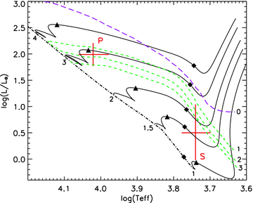
HR diagram of V380 Ori. The red crosses are the error bars in temperature and luminosity of the primary (labelled P), and the secondary (labelled S). The PMS evolutionary tracks of 1, 1.5, 2, 3 and 4 M⊙ are plotted using full lines. The ZAMS (dot–dashed line); the isochrones (green dashed lines) of 1, 2 and 3 Myr; and the birthline (blue long dashed line), calculated with a mass accretion rate of 10−5 M⊙ yr−1 by Palla & Stahler (1993), are also plotted. The filled diamonds indicate the moment where the mass of the convective envelope becomes lower than 1 per cent of the stellar mass and the triangles indicate the appearance of the convective core.
Fundamental parameters of the primary and secondary components of V380 Ori. Columns 2–5 give the effective temperature, the luminosity, the mass and the radius of the stars, respectively. Column 6 gives the age of the system. The projected rotational velocities (v sin i– derived in Section 4.2) are given in Column 7. The macroturbulent velocity (vma– also derived in Section 4.2) of the primary is indicated in Column 8. vma of the secondary cannot be derived using our data. The 2σ uncertainties are indicated.
| Star | Teff (K) | log(L/L⊙) | M/M⊙ | R/R⊙ | Age (Myr) | v sin i (km s−1) | vma (km s−1) |
| P | 10500 ± 500 | 1.99 ± 0.22 | 2.87+0.52−0.32 | 3.0+1.1−0.8 | 2 ± 1 | 6.7 ± 1.1 | 3.5 ± 0.8 |
| S | 5500 ± 500 | 0.50+0.54−0.56 | 1.6+1.0−0.6 | 2.0+1.8−0.9 | 18.7 ± 3.2 |
| Star | Teff (K) | log(L/L⊙) | M/M⊙ | R/R⊙ | Age (Myr) | v sin i (km s−1) | vma (km s−1) |
| P | 10500 ± 500 | 1.99 ± 0.22 | 2.87+0.52−0.32 | 3.0+1.1−0.8 | 2 ± 1 | 6.7 ± 1.1 | 3.5 ± 0.8 |
| S | 5500 ± 500 | 0.50+0.54−0.56 | 1.6+1.0−0.6 | 2.0+1.8−0.9 | 18.7 ± 3.2 |
4.2 Calculation and fitting of the least-squares deconvolved Stokes I profiles
In order to increase the S/N of our data, to measure accurate rotational and radial velocities of both stars and to constrain their magnetic field characteristics, we applied the LSD method (Donati et al. 1997) to our spectra using two different line masks (describing the positions, relative intensities and Landé factors of all lines predicted to be present in the spectrum): one for the primary component and one for the secondary. Both masks have been calculated using the stellar atmosphere code atlas9 of Kurucz (1993) for the temperatures and gravities of both stars determined in Section 3.1. The masks have been cleaned as follows. For each star, we have selected lines that are not blended with the other component at any time and that are not contaminated by emission, and we have rejected all other lines, including the Balmer lines. The resulting masks contain 85 and 374 lines, respectively, for the primary and the secondary components. The number of lines in the mask of the secondary is larger than in the primary mask due to its lower temperature and also due to the fact that the spectrum of the secondary shows less contamination by emission.
The results of this procedure were two sets of 24 Stokes I, V and diagnostic N LSD profiles, for the primary and secondary, respectively. The peak S/N in the Stokes V profiles, indicated in Table 1, are higher in the secondary profiles than in the primary's due to a larger number of lines in the secondary mask.
To determine the radial velocity (vrad) and the projected rotational velocity (v sin i) of both stars, we performed a simultaneous least-squares fit to the 24 LSD Stokes I profiles, independently for each star. Each profile was fitted with the convolution of a rotation function (for which the projected rotational velocity v sin i is a free parameter in the fit) and a Gaussian whose width is computed from the spectral resolution and a macroturbulent velocity (Gray 1992).
The free parameters of the fitting procedure are the centroids, depths, v sin i and macroturbulent velocity vma of each component. The centroids of the functions can vary from one profile to another, whereas the depths, v sin i and vma, of each component cannot. This fitting procedure therefore assumes that the depths, v sin i and vma of both components do not vary with time, which we confirm (within the error bars) by fitting each profile separately. Including the macroturbulent velocity as a free parameter in the fit of the secondary profiles results in a macroturbulence consistent with zero, but with a very large error bar. As the S/Ns of the secondary profiles are very low, we therefore conclude that this parameter cannot be constrained by fitting these profiles. Therefore, for the fit of the secondary profiles, vma has not been considered as a free parameter and has been fixed at 0 km s−1.
Figs 7 and 8 show the resulting fits superimposed on the observed Stokes I profiles of the primary and the secondary components, respectively. The profiles of 2007 November 6 and 11 have not been taken into account in the secondary fit because these profiles contain, in the red wing, a strong absorption component whose origin is unknown. Including them in the fit results in a poorer fit and in larger error bars. We also observe that the depths of some profiles of the secondary are not well reproduced, which might be due to variable circumstellar emission or absorption contaminating some spectral lines at few observational dates. However, the strongest differences observed between the fit and the observed profiles are within the error bars. Therefore, considering the complexity of the spectrum of the system, the mask used to compute these LSD profiles gives a satisfactory result.
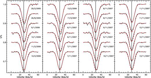
LSD Stokes I profiles of the primary star V380 Ori A, calculated from the 24 observed spectra (black full lines), superimposed with the best fit (red dashed line) described in Section 4.2. The dates of the observations are indicated beside each profile.
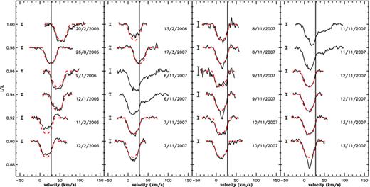
LSD Stokes I profiles of the secondary star V380 Ori B, calculated from the 24 observed spectra (black full lines), superimposed with the best fit (red dashed line) described in Section 4.2. The dates of the observations are indicated beside each profile. The profiles of 2007 November 6 and November 11 show an absorption component in the red wing, whose origin is unknown. Therefore, these profiles have not been included in the fit.
This automatic fitting procedure enables us to measure the v sin i and radial velocities of both components. We obtain projected rotational velocities of 6.7 ± 1.1 and 18.7 ± 3.2 km s−1 for the primary and the secondary components, respectively, and a macroturbulent velocity for the primary of 3.5 ± 0.8 km s−1. The radial velocities of both components are included in Table 1 and are analysed in the next section.
4.3 The radial velocity variations
The separation between the primary and the tertiary being 200 times larger than the separation between the primary and the secondary, in the following, we will treat the system as a binary system, and we will ignore the impact from the IR companion in the radial velocity analysis.
As mentioned in Section 3.3.1, the radial velocities of the spectral lines of the secondary vary with time, while those of the primary do not. The radial velocities of the components, measured using the LSD Stokes I profiles, confirm this observation. We have fitted the temporal variation of the radial velocities of both components assuming a circular orbit. We should note that we also succeeded in fitting these variations using an eccentric orbit. However, the uncertainties are sufficiently large that we have no indication that these orbits are eccentric, and we will only consider the simplest model that can reproduce our measurements.
As the radial velocity of the primary does not vary significantly, we chose to include the measurements into the fit as a constant with time equal to the systemic radial velocity, in order to better constrain this parameter. We performed a simultaneous fit of both radial velocity curves using simple sinusoids for each curve. This fitting procedure depends on four parameters: the orbital period (Porb) of the system, the reference time (T0), the systemic radial velocity (γ) and the radial velocity amplitude of the secondary (KS). We determined an upper limit on the radial velocity amplitude of the primary (KP) using the mean of the error bars of the measurement of its radial velocity.
The radial velocities of both components, and the result of the fit of the orbits, are plotted in Fig. 9, folded with the orbital period. The values of the fitting parameters are presented in Table 3. We derive only a lower limit on the mass ratio MP/MS of 2.9, consistent, within the error bars, with the mass ratio obtained from the HR diagram in Section 4.1(MP/MS= 1.8+1.6−0.8). Using the masses derived from the HR diagram, and the inferred value of MP sin3iorb and MS sin3iorb, we find that the inclination angle between the orbit axis and the observer's line of sight (iorb) is lower that 31°, using the primary mass, and lower than 13°, using the secondary mass, which indicates that the orbit might be seen close to pole-on. Due to the relatively low S/N of our data, the uncertainties on the orbits and fundamental parameters of the stars are large. More spectroscopic observations of a higher S/N are required in order to better constrain the orbital parameters and the mass ratio of the system.
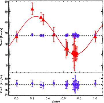
Radial velocities of the primary (blue points) and the secondary (red triangle) plotted as a function of the orbital phase (according to the ephemeris given in Table 3) and superimposed with the best-fitting radial velocity curve of the secondary. The systemic radial velocity is indicated with a black dashed line. The lower panel shows the radial velocities of the primary on a smaller scale.
Orbital parameters of the system. a is the distance between both stars. aP and aS are the radii of the primary and the secondary (circular) orbits, respectively. iorb is the inclination angle between the orbit axis and the line of site of the observer. KP has not been determined within the fitting procedure, but from the error bars of the radial velocities of the primary. The 3σ error bars are indicated.
| Results of the fit | |
| Period (d) | 104 ± 5 |
| T0 (HJD) | 245 3505 ± 18 |
| γ (km s−1) | 27.8 ± 2.1 |
| KS (km s−1) | 18 ± 14 |
| KP (km s−1) | <1.4 |
| Derived parameters | |
| MP/MS | >2.9 |
| a sin iorb (au) | <0.33 |
| aP sin iorb (au) | <0.0139 |
| aS sin iorb (au) | 0.17 ± 0.14 |
| MP sin3iorb(M⊙) | <0.40 |
| MS sin3iorb(M⊙) | <0.018 |
5 MAGNETIC FIELD ANALYSIS
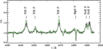
Fig. 10 shows the LSD Stokes I, V and diagnostic N profiles of the primary (left) and the secondary (right) for one night, calculated using the masks described in Section 4.2. We observe that the null N profile is totally flat in both cases, indicating that the signature observed in the Stokes V profile of the primary is real, and is not a spurious signal created by instrumental artefacts. The magnetic field detection in the primary is furthermore confirmed by the detection of Zeeman signatures in the Hα line and in each line of the triplet O i 777 nm (Wade et al. 2005). Unlike the primary, the Stokes V profile of the secondary does not show any Zeeman signature, meaning that no magnetic field has been detected at the surface of the star. It also confirms that the mask of the secondary does not contain lines contaminated with lines from the primary.
LSD Stokes I, V and diagnostic N profiles of the primary (left) and the secondary (right), normalized to the continuum of the binary Ic. These profiles have been obtained from the first 2007 November 12 spectrum. The mean error bars are indicated beside each profile. The V and N profiles have been shifted vertically and have been multiplied by a factor of 3 for the primary and 2 for the secondary, for display purpose.
5.1 Phased longitudinal field variation of the primary
In order to characterize the magnetic field of the primary, we need to model the Stokes I and V profiles. The magnetic fields of the Ap/Bp stars and of the other field HAeBe stars are large-scale organized fields, with an important dipole component. We therefore used the oblique rotator model, that is a dipole of polar strength Bd placed at the centre of the star, with a magnetic axis inclined at an angle β with respect to the rotation axis and the line of sight making an angle i with the rotation axis (Landstreet 1970). As the star rotates with a period P, the magnetic configuration on the observed surface of the star changes with time. Therefore the Stokes V profile, and the magnetic strength projected on to the line of sight and integrated over the observed surface, that is the longitudinal magnetic field (Bℓ), change with time.
P, the rotation period of the star;
t0, the reference Julian Date of maximum of Bℓ;
B, the semi-amplitude of the curve;
B0, the vertical shift of the sinusoidal curve with respect to Bℓ= 0;
consistent with the oblique rotator model. The best-fitting model, superimposed on the data in Fig. 11, gives the following parameters: P= 4.43 ± 0.23 d,  d, B= 440 ± 200 G, B0= 0 ± 140 G, with χ2= 1.4. In contrast, the χ2 calculated assuming a zero-field model (in which the longitudinal magnetic field is constant and equal to 0) is 11.3.
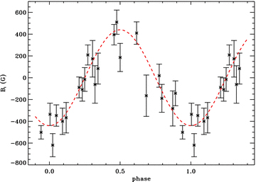
Longitudinal magnetic field (Bℓ) of the primary plotted as a function of the rotation phase, according to the ephemeris summarized in Section 5.1. The best-fitting sinusoid is also plotted as a red dashed line. The data points for both 2007 November 9 observations (with relatively large error bars) have been removed from the plot, for display purpose.
The detailed measurements of the longitudinal magnetic field values depend sensitively on the integration range used in the calculation of the first moment of V and the equivalent width. We have measured Bℓ for numerous integration ranges, by varying the blue limit from 0 to 18 km s−1, and the red limit from 40 to 60 km s−1. We find that the standard deviation of the values of Bℓ measured from a single LSD profile can be as high as 285 G. Furthermore, the measured values for two profiles observed on the same night can show important differences as large as 700 G, while the Stokes V profiles do not show any significant difference. These effects can have important consequences for the determination of the amplitude of variation B as well as the shift of the sinusoid B0. In contrast, however, whatever the integration range used, the Bℓ values show similar variations with a periodicity around 4.4 d, implying that the determination of the period is insensitive to the integration range. These characteristics have already been observed during our previous analysis of the magnetic HBe star HD 200775 (Alecian et al. 2008). As for HD 200775, we will not try to determine the magnetic geometry of V380 Ori A using the longitudinal magnetic field, and we will determine it by fitting directly the Stokes V variations, using the period derived in this fit as a first guess in the Stokes V modelling. We should note that Fig. 11 shows that the phase coverage is uniform and complete, which is optimal for modelling the magnetic topology of the star.
5.2 Fitting of the Stokes V profiles of the primary
The observed Stokes V profiles are plotted in black full lines in Fig. 12. We see clear variations indicating rotational modulation of the magnetic field at the visible surface of the star. To fit the Stokes V profiles directly, we use the dipole oblique rotator model described above. Using the relations of Landstreet (1970), giving the intensity of the magnetic field at each point on the stellar surface, we calculate the longitudinal magnetic field bℓ(θ, ϕ), at each point (θ, ϕ) of the surface of the star, in classical spherical coordinates in the observer's frame.

LSD V profiles of the primary (full black lines) superimposed by the best oblique rotator model (dashed red line). The numbers close to the profiles are the rotation phase and the small bars on the right of the profiles are the mean error bars in V. The profiles are sorted by an increasing rotational phase and the date of observation is indicated next to each profile.
 and λ0 (Å) are the mean Landé factor and wavelength of the lines used in the mask (Section 2), respectively, c is the speed of light, I(θ, ϕ) is the local intensity profile and v is the local radial velocity due to stellar rotation. Then we integrated over the visible stellar surface using the limb-darkening law with a parameter equal to 0.5 (Claret 2000). We obtain the synthetic Stokes V(v) profile, that we normalize to the intensity continuum, to compare to the observed V profiles. This model depends on the following five parameters:
P, the rotation period;
t0, the reference Julian Date of the maximum of the surface magnetic intensity, used with P to compute the rotation phase;
i, the inclination of the stellar rotation axis to the observers line of sight;
β, the magnetic obliquity angle;
Bd, the dipole polar magnetic intensity.
We calculated a grid of V profiles for each date of observation (see Table 4 for details on the grid), varying the five parameters and assuming for the initial value of P the solution obtained from modelling the longitudinal field variation. Then we applied a χ2 minimization to find the model which best matches simultaneously our 24 observed profiles. The best model that we found, with χ2= 1.6, corresponds to P= 4.312 76 ± 0.000 42 d, i= 32°± 5°, β= 66 ± 5 and Bd= 2120 ± 150 G, where the error bars correspond to the 3σ confidence level (Table 5). Fig. 12 shows the synthetic Stokes V profiles superimposed on the observed ones. We see that this model acceptably reproduces most of the observed V profiles.
Ranges and minimum bins of parameters explored in the fit of the Stokes V profiles.
| Parameters | Min | Max | Bin |
| P (d) | 3.0 | 5.0 | 0.000 01 |
| T0 (HJD) | 24 3510 | 245 3515 | 0.001 |
| i (°) | 0 | 180 | 0.1 |
| β (°) | 0 | 180 | 0.1 |
| Bd (G) | 0 | 6000 | 10 |
| Parameters | Min | Max | Bin |
| P (d) | 3.0 | 5.0 | 0.000 01 |
| T0 (HJD) | 24 3510 | 245 3515 | 0.001 |
| i (°) | 0 | 180 | 0.1 |
| β (°) | 0 | 180 | 0.1 |
| Bd (G) | 0 | 6000 | 10 |
Magnetic dipole model of V380 Ori A. The 3σ error bars are indicated.
| P (d) | 4.312 76 ± 0.000 42 |
| T0 (HJD) | 245 4412.997 ± 0.043 |
| i (°) | 32 ± 5 |
| β (°) | 66 ± 5 |
| Bd (G) | 2120 ± 150 |
| P (d) | 4.312 76 ± 0.000 42 |
| T0 (HJD) | 245 4412.997 ± 0.043 |
| i (°) | 32 ± 5 |
| β (°) | 66 ± 5 |
| Bd (G) | 2120 ± 150 |
The period found using this fitting procedure is consistent with that derived from the longitudinal magnetic field variation. However, neither i nor β is close to 90°, a result which is inconsistent with the symmetry of the longitudinal magnetic field variation with respect to Bℓ= 0 . However, the amplitudes of the Stokes V profiles around phases 0 and 0.5 are clearly different, leading to different absolute values of the longitudinal magnetic fields. From these simple observations, we therefore do not expect a symmetric longitudinal magnetic field curve. We are therefore confident with the magnetic configuration found using the fitting of the Stokes V profiles, and we confirm that using Bℓ values obtained from low S/N data is unreliable for determining the detailed magnetic configuration of a star.
5.3 Stokes V analysis of the secondary
We used the Stokes I and V profiles of the secondary star to determine the upper limit on the strength of a magnetic field that the star could host. According to the position of the secondary in the HR diagram (Fig. 6), its PMS evolutionary status is not well defined. The star might possess a convective envelope under the surface that could give rise to magnetic fields of a complex structure through a convective dynamo as in the T Tauri stars. Therefore, we do not claim that this star hosts a large-scale organized magnetic field; however as no magnetic field has been detected we will assume the simplest model, which is the oblique rotator model as described above.
Our method consists of calculating simulated Stokes V observations of the same S/N as our data. For each one of the 24 LSD profile sets, and for a fixed value of the dipole strength Bd, we have calculated 100 simulated Stokes V profiles as follows. For each of the 100 iterations, we adopted random values of i and β. We then computed 24 synthetic Stokes V profiles using the oblique rotator model, assigning a random phase to each LSD profile. In this calculation we used a Stokes I profile computed with the v sin i, central depth and macroturbulent velocity found in Section 4.2, a radial velocity equal to 0 km s−1 and a limb-darkening coefficient of 0.7 (Claret 2000). To the computed Stokes V profiles, we then added synthetic Gaussian noise consistent with the S/N of the observations. For each of these simulated profiles, we calculated the detection probability (Donati et al. 1997). We consider that a magnetic field would have been detected at 3σ if the detection probability is greater than 0.9973. We calculated the number of iterations that gives at least one 3σ detection among the 24 simulated profiles, and we repeated this procedure for different values of Bd. We find that if Bd is greater than 800 G, the probability of having at least one detection among our data is 99 per cent, while if Bd is greater than 500 G this probability is 90 per cent. Therefore, if the secondary hosts a dipole at its centre, its strength is very likely to be below 500 G.
6 DISCUSSION AND CONCLUSIONS
This paper describes the analysis of high-resolution spectropolarimetric observations of the PMS Herbig Ae star V380 Ori, obtained with the new generation instruments ESPaDOnS and Narval. The main goal of this study was to characterize the stellar magnetic field discovered in 2005 (Wade et al. 2005) and to further explore the origin of the magnetic fields of intermediate-mass stars. The results of the analysis are summarized and discussed below.
First, a careful investigation of the intensity spectrum of V380 Ori led to the discovery of a cool spectroscopic companion and confirmed the detection of the Li i 6707 Å line reported by previous authors. We argue that this spectroscopic companion cannot be the IR companion discovered by Leinert et al. (1994), which implies that V380 Ori is a triple system with two spectroscopic components and an IR companion.
The modelling of the binary spectrum allowed the determination of the effective temperatures of both stars, as well as the luminosity ratio of the system, and revealed a high metallicity ([M/H]= 0.5) of the primary. The same metallicity was also able to reproduce the lines of the secondary, but was not required to obtain an acceptable fit of its spectrum. As a magnetic field has been discovered only in the primary, we therefore proposed that the primary is a magnetic chemically peculiar star, as observed among the magnetic A/B star on the MS. No variability is observed in the shape and strength of the lines, implying that any non-uniformities in the surface distribution of Fe and Ti are either too small to be detected or that these elements are distributed symmetrically about the rotation axis. These results, if confirmed with more accurate observations and a thorough study of the abundances, would give the first Herbig Ae star, whose environment is highly dense, that is able to develop abundance anomalies at its surface. It would also lead to unique constraints on the physical processes at the origin of these anomalies and the time-scales for developing them, as well as constraints on the interaction of the star with its environment in the presence of a strong magnetic field.
The intensity spectrum was found to be strongly contaminated with emission. The emission in the metallic lines is correlated with the central depth and the excitation potential of the lines: at constant excitation potential, the greater the central depth, the greater the emission, while at constant central depth, the greater the excitation potential, the lower the emission. The strongest emission, observed mainly in the Fe ii and Ti ii lines, shows three sub-structures, each of which was well reproduced with a Gaussian function. The fit of these lines revealed the following.
A main emission component with a constant FWHM of ∼65 km s−1 over the spectrum and over time, slightly redshifted compared to the radial velocity of the primary.
Two wing emissions, one in each wing of the main emission component, whose amplitude and broadening vary with time, that might come from a disc surrounding the central star.
We argued that these emissions are very likely produced in a circumbinary disc whose emission properties are mainly driven by the primary's light and might not be contaminated with the emission of the secondary. However, the three components of the system might contribute to the strong emission profiles of a complex structure and variability observed in the Balmer lines. Our data did not allow us to determine any correlation between the temporal variations of the wing emission components and the rotation period of the primary star. We are therefore unable to assess whether the proposed disc surrounding the primary is produced by magnetic confinement, as proposed by Townsend, Owocki & Groote (2005), to explain the disc surrounding the hotter MS Bp star σ Ori E. On the other hand, the lack of veiling (associated with accretion shock hotspots), the lack of correlation between the rotation period and emission variability, and the absence of distortion in the Stokes I profiles (signs of hot or cold spots) suggest that magnetospheric accretion is not occurring around the primary star, as one might expect from its PMS status and the similarity between its emission spectrum and those of the T Tauri stars.
The strong similarity of the characteristics of the emission lines between V380 Ori and HD 190073 is puzzling. If the main emission component is arising in a disc, we would expect to measure different FWHMs of their emission profile, due to different inclination angles. The probability of observing two magnetic HAe stars under the same angle being very low, the main emission component might come from another forming region with isotropic properties. As in Catala et al. (2007) we can consider the scenario of a heated region at the base of a wind arising from the photosphere, with turbulent motions. However, the problem encountered with HD 190073 is also encountered with V380 Ori: most of the emission lines are redshifted with respect to the radial velocity of the star, while we would expect them to be blueshifted if they come from a wind. The similarity of the emission spectrum of both stars therefore puts very strong constraints on the physical and geometrical properties of their circumstellar environment.
The P Cygni absorption observed in Hα and in the Ca H and K lines revealed the presence of a wind surrounding either the central star or the central binary. The shape, radial velocity and broadening of all these emissions showed strong variations on time-scales of days, and sometimes hours, suggesting a vigorous dynamic in the environment of the stars. More observations of a better S/N coupled with linear polarimetric and interferometric data, and compared to models of circumstellar discs and winds, would be required in order to conclude about the circumstellar geometry and the physical processes involved in the formation and the dynamic of these emissions.
Using the LSD Stokes I profiles of both components, we determined their projected rotational velocities and radial velocities. We modelled the variations of the radial velocities of both stars and determined the orbital parameters and the mass ratio of the system. As no variations are observed in the radial velocity of the primary, only a lower limit was determined on the mass ratio, a value that is consistent with the mass ratio determined using the HR diagram.
The LSD Stokes V profiles of the primary show a clear Zeeman signature characteristic of an organized magnetic field at the surface of the star. We found that the oblique rotator model of a centred dipole was able to reproduce acceptably the temporal variations of the Stokes V profiles, implying that the large-scale magnetic field of V380 Ori A is a simple dipole, as observed in the other HAeBe stars and in the Ap/Bp stars. The result reinforces arguments in favour of a fossil magnetic origin by showing that there is no exception to the apparent rule that all magnetic intermediate-mass stars host large-scale, organized magnetic fields.
The fit of the Stokes V profiles led to an inclination of the rotation axis equal to 32°± 5°. However, assuming rigid rotation and using the derived rotation period of 4.312 76 ± 0.000 42 d, the radius inferred from the HR diagram position, and the v sin i measured from the LSD Stokes I profiles, we infer i= 11+7−4°, which is inconsistent with the determination from the Stokes V fit. In order to understand this difference, we performed different tests. First, we fixed the inclination angle to 11° and performed a new fit on the Stokes V profiles. The result produced synthetic Stokes V profiles inconsistent with the observed ones around phase 0.0. Secondly, the plot of the χ2 as a function of the period shows several local minima, and therefore we searched for the best magnetic configuration, reproducing the Stokes V profiles around the periods associated with the local minima. In each case, the synthetic profiles were found to be inconsistent with the observed profiles. However, the magnetic strength inferred when we performed these tests remained very close to our final determination (Bd= 2100 G). We therefore conclude that the magnetic configuration and the rotation period that we find using the fit of the Stokes V profiles is robust and is not the source of the disagreement between both values of the inclination angle.
This disagreement might come from the determination of the radius of the primary, inferred from the effective temperature and the luminosity of the star. While we are confident with the determination of the temperature within the error bars, our determination of the luminosity is more debateable. The error bars on the luminosity are determined from the uncertainties on the distance and the luminosity ratio (LP/LS). We did not take into account the fact that the star is variable, as well as the uncertainty on the interstellar extinction, which might lead to additional uncertainties. We encountered the same problem during our study of HD 200775: an inconsistency between two different determinations of the inclination (Alecian et al. 2008). As for HD 200775, we must conclude that the determination of the luminosity of HAeBe stars, as well as the fundamental parameters using the HR diagram, are highly uncertain, and must be used with caution.
If the luminosity that we determined is overestimated, the inferred mass and radius of the primary might be also overestimated. Using our estimation of the mass and using the PMS stellar evolutionary models, we can determine the radius of the primary when it will reach the zero-age MS (ZAMS). Notwithstanding that our estimates of masses and radii of the components are highly uncertain, we can reasonably assume that the ZAMS radius of a 10 500 K star is greater than 2 R⊙. Using our determination of the radius, and the fact that we might have overestimated it, the upper limit on the actual radius is 4 R⊙. We therefore deduce that the ratio of the actual radius to the ZAMS radius is not larger than 2 and can be as low as 1. Using this range of R/RZAMS, we can derive the magnetic strength and the period on the ZAMS.
Assuming magnetic flux conservation during the PMS phase, we predict that, when the primary will reach the MS, its magnetic strength will be larger than ∼2 kG, which is of the same order of magnitude as the magnetic strengths of the Ap/Bp stars, as expected in the context of the fossil model. Assuming the conservation of angular momentum, we find that the rotation period on the ZAMS can be as low as 1.1 d, similar to the rotation periods of the Ap/Bp stars (>1 d), meaning that V380 Ori A might evolve towards the ZAMS with a constant angular momentum.
Assuming that i= 32°, the true equatorial velocity of the primary is estimated to be 13 km s−1, showing that V380 Ori A is already a slow rotator at an age around 2 Myr. In order to explain the slow rotation observed among the Ap/Bp stars, Stȩpień (2000) proposed that magnetic braking occurs during the PMS phase of stellar evolution. As V380 Ori A already appears to have lost significant rotational angular momentum, our results show that if this star experienced a braking mechanism it must have been during the very first stages of the PMS evolution, or before.
Using simulated observations of Stokes V profiles of the secondary, calculated from the oblique rotator model, we determined an upper limit of 500 G (at 90 per cent confidence) on any dipolar magnetic field that this star may host. If the fossil model is correct, one would expect that a binary system should be composed of two magnetic stars with a similar magnetic flux, if both stars have formed from the same molecular cloud (which is a reasonable hypothesis considering the young age of this system). Using the radii determined in Section 4.1, we find an upper limit of 145 kG R2⊙ on the magnetic flux (Bd×R2) of the secondary and a lower limit of 100 kG R2⊙ for the magnetic flux of the primary, which means that our results are consistent with the fossil field hypothesis. However, the radii of the stars are very poorly constrained. In order to better constrain the fossil model, we need to improve the determination of the fundamental parameters of both stars by performing interferometric observations and measuring separately both luminosities. However, the instrumentation available today is limited to bright magnitudes and will not be able to resolve the stars. In a few years, once the efficiency of the interferometers has improved, these observations will be feasible and could be leaveraged to bring new constraints to test the fossil hypothesis.
We deeply thank Mathieu Vick, Georges Michaud, Georges Alecian and Pierre Kervella for fruitful discussions. We are very grateful to O. Kochukhov, who provided his binmag1 code. We really appreciate our exchanges with Jerome Bouvier regarding his results on high-resolution imaging data of V380 Ori. EA is supported by the Marie Curie FP6 program. GAW and JDL acknowledge support from the Natural Science and Engineering Research Council of Canada (NSERC). GAW further acknowledges DND (Canada) Academic Research Programme (ARP). We warmly thank the referee, A. Hatzes, for his judicious comments.
REFERENCES
Author notes
Based on observations obtained at the Canada–France–Hawaii Telescope which is operated by the National Research Council of Canada, the Institut National des Sciences de l'Univers of the Centre National de la Recherche Scientifique of France and the University of Hawaii.
Based on observations obtained at the Bernard Lyot Telescope (Pic du Midi, France) of the Midi-Pyrénées Observatory, which is operated by the Institut National des Sciences de l'Univers of the Centre National de la Recherche Scientifique of France.
