


Abstract
We present a study of a sample of Large Magellanic Cloud red giants exhibiting Long Secondary Periods (LSPs). We use radial velocities obtained from VLT spectral observations and MACHO and OGLE light curves to examine properties of the stars and to evaluate models for the cause of LSPs. This sample is much larger than the combined previous studies of Hinkle et al. and Wood, Olivier & Kawaler.
Binary and pulsation models have enjoyed much support in recent years. Assuming stellar pulsation, we calculate from the velocity curves that the typical fractional radius change over an LSP cycle is greater than 30 per cent. This should lead to large changes in Teff that are not observed. Also, the small light amplitude of these stars seems inconsistent with the radius amplitude. We conclude that pulsation is not a likely explanation for the LSPs. The main alternative, physical movement of the star – binary motion – also has severe problems. If the velocity variations are due to binary motion, the distribution of the angle of periastron in our large sample of stars has a probability of 1.4 × 10⁻³ that it comes from randomly aligned binary orbits. In addition, we calculate a typical companion mass of 0.09 M⊙. Less than 1 per cent of low-mass main-sequence stars have companions near this mass (0.06–0.12 M⊙) whereas ∼25–50 per cent of low-mass red giants end up with LSPs. We are unable to find a suitable model for the LSPs and conclude by listing their known properties.
1 INTRODUCTION
A subset of Long-Period Variable stars (LPVs) was found several decades ago to show a secondary period of variation, in addition to their primary pulsation (e.g. Payne-Gaposchkin 1954; Houk 1963). These Long Secondary Periods (LSPs) exceed the primary period in length by approximately one order of magnitude, a fact more recently confirmed by Wood et al. (1999). Wood et al. showed that LPVs fall on four distinct period-luminosity sequences A–D, and they found an additional sequence, E, of red giant binaries. These multiple sequences have been confirmed in subsequent studies, and a splitting of sequence B into two sequences has since been discovered (Ita et al. 2004; Soszyński et al. 2004a; Fraser et al. 2005; Soszynski et al. 2007). LSPs occupy sequence D, the sequence corresponding to variations with the longest period. The primary pulsation of these stars is usually found on sequence B (Wood et al. 1999).
Approximately 25–50 per cent of LPVs show an LSP (Wood et al. 1999; Percy et al. 2004; Soszyński et al. 2004b; Soszynski et al. 2007; Fraser, Hawley & Cook 2008). At present, there is no accepted explanation for LSPs. Wood et al. (1999) initially proposed a model wherein the sequence D stars are semi-detached red giant binaries, as the length of their periods are consistent with those expected for binary systems with solar-mass components. Several other models have been proposed to explain LSPs, including radial and non-radial pulsation, and dust effects. However, Wood et al. (2004) demonstrate that there are problems with all of these models. It is clear that further investigation is required in order to discover the cause of LSPs.
Here, we study a sample of sequence D stars in the Large Magellanic Cloud (LMC) in order to provide new constraints on models for the sequence D phenomenon. In particular, we present new spectra taken with the European Southern Observatory's Very Large Telescope (VLT). We derive velocity curves, radii and effective temperatures from these spectra and compare them in phase with light curves and associated quantities from the MACHO (Alcock et al. 1992) and OGLE (Udalski et al. 1992) data bases.
Our study follows the methods of Hinkle et al. (2002) and Wood et al. (2004), who also compared both light and radial velocity data for sequence D stars. However, we use a larger data set and have the advantage of high quality and simultaneous light and velocity data, which we hope will give a more complete and accurate picture of the behaviour of LSP variables. Since our sample comes from the LMC, we also have the advantage that the distances, and hence derived luminosities, are well determined.
2 OBSERVATIONS AND DATA REDUCTION
We chose a region of high star density in the middle of the LMC bar for this study, in order to get a large sample of sequence D stars in the 20 arcmin field of the FLAMES (Pasquini et al. 2002) multifibre system on the VLT. The field centre is at 05h28′15″−69°45′43″ J2000. It contained a sample of 58 variable red giants exhibiting LSPs which were obtained from the MACHO Project data base. It was important to have simultaneous light and velocity data. Fortunately, OGLE light curves were taken at the times of our VLT observations. We have used both OGLE II and OGLE III I-band light curves in this study.
Spectra were obtained on 21 nights from 2003 November to 2006 March. The FLAMES/GIRAFFE spectrograph (Pasquini et al. 2002) with a grating setting of HR16 was used, giving spectra with a resolution of 23 900 and a spectral interval of 693.7–725.0 nm. This region includes the TiO bandhead at 705 nm, which can be used for spectral typing and to examine variation of Teff, as well as derivation of radial velocities. An exposure time of 20 min was used for all spectra. The spectra were obtained in service mode. Unfortunately, no observations were taken between May and August when the LMC (RA =05h23′) was only observable near twilight, leaving a long winter gap in 2004 and 2005.
The raw spectra of the 58 sequence D stars, most of which have 21 observations from different dates, were reduced using the FLAMES/GIRAFFE pipeline or the Swiss reduction pipeline. A number of sample spectra are shown in Fig. 1, where the TiO bandhead is clearly visible in the second and third panels. The majority of the program stars have spectra similar to those shown in the top three panels, i.e. they are oxygen-rich giants of spectral types M and K. However, the sample does contain a number of carbon-rich stars (C-stars), as shown in the fourth panel of Fig. 1.
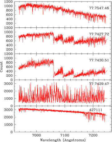
Sample spectra from the VLT. Top panel: the spectrum of an O-rich program star with no TiO bands. Second panel: a program star with weak TiO bands. Third panel: a program star with strong TiO bands. Fourth panel: a C-rich program star. Bottom panel: a telluric star. Program stars are identified by their MACHO numbers. Note the different scale of the y-axis in the lower two panels.
Using the iraf software, each spectrum was visually examined and any obvious cosmic rays removed. There was a small percentage of bad data: in particular, spectra taken on two dates (2005 March 17 and 2005 September 10) had very few counts. This was due to the weather and seeing conditions at the time, and the spectra taken on these dates were discarded, leaving 19 good observations for most stars (some stars had fewer spectra due to the fibre allocation process in FLAMES). A small number of other spectra were discarded due to a low number of counts. These spectra did not fall on particular dates or particular target stars, and were distributed randomly throughout the data set. Presumably, the low counts were due to the fibres for these stars being misaligned.
Relative radial velocities were obtained through cross-correlation with the iraf task fxcor. From each star, a spectrum with a high number of counts and narrow lines was selected, and this acted as the template spectrum for the star's cross-correlation. The cross-correlation was performed in the wavelength region 6950–7160 Å, as this region is relatively free of telluric lines, as can be seen in the lower panel of Fig. 1. Errors in the radial velocities were also taken from fxcor. The mean velocity error of the sample is 0.42 km s−1, and errors typically range between 0.1 and 0.6 km s−1.
Because of uncertainty about the accuracy of the velocity calibration resulting from the pipeline reduction, the spectra were checked to see if any zero-point correction to the velocity was needed, before we calculated their absolute velocities. This procedure is now described.
2.1 Testing the relative telluric radial velocities
To check the velocity calibration, program stars were cross-correlated with a B star whose spectrum contained only telluric lines. Cross-correlation of a program spectrum to a telluric spectrum produces the relative telluric velocity of the two spectra, which should be zero if there are no calibration errors. This cross-correlation was performed in the wavelength region 7160–7220 Å, as it has a large concentration of telluric lines (see Fig. 1).
For most dates of observation, the relative telluric radial velocities were found not to be significantly different from zero, and so no systematic correction was applied to the spectra for those nights. However, observations from two nights, with Heliocentric Julian Dates (HJD) of 2453377 and 2453643, consistently showed a positive velocity offset from zero, so a zero-point correction for the velocities on these dates was included for all stars. The velocity corrections for these dates were −2.061 and −0.729 km s−1, respectively.
2.2 The effect of telluric lines on relative radial velocities
The highest concentration of telluric lines was found in the wavelength region 7160–7220 Å, but there were a small number in the program object region (6950–7160 Å, see Fig. 1). There was a possibility that these lines would affect the calculated radial velocities, so this was examined. The telluric lines in the program object region of several program stars were removed using iraf's telluric command. Then the program spectra with telluric lines removed were cross-correlated against each other in the same way the original program spectra were. It was found that removing the telluric lines in this region had no significant effect on the velocities or errors, so telluric line removal was not performed.
2.3 Calculating the absolute radial velocity
Following the zero-point corrections, the absolute radial velocities of the program stars were calculated. First, the template of each program star was cross-correlated to a star of known radial velocity, giving the absolute radial velocity of each template. Then by adding a keyword ‘vhelio’ (which contained the absolute radial velocity) to the image header of the template, we could cross-correlate the spectra for each star with its template to obtain the absolute radial velocities.
For the O-rich program stars, the radial velocity reference used was α Cet. Its spectrum was taken using the echelle spectrograph (resolution 70 000) on the late 74-inch telescope at Mount Stromlo Observatory, Canberra, Australia. For the C-stars, the reference used was the C-star X Vel, for which a spectrum was also taken with the 74-inch. The radial velocity used for α Cet was −25.8 km s−1 (taken from the Astronomical Almanac, Tettelbach & Holdaway 2004). The velocity for the spectrum of X Vel (−5.4 km s−1) was obtained by cross-correlation with α Cet (even though the spectral types are different, there was a strong cross-correlation peak due to common metal lines).
Radial velocities as a function of heliocentric Julian date (HJD) for a sample of the sequence D stars are shown in Table 1. Stars are identified by their MACHO numbers. Dashes denote dates for which there is no spectrum. The full table can be viewed in the online version of this paper (see Supporting Information).
Heliocentric radial velocities of sequence D Stars (km s−1). The full table can be viewed in the online version of the paper (see Supporting Information).
| HJD | 77.7427.41 | 77.7427.72 | 77.7428.120 | 77.7428.65 | 77.7429.100 | 77.7429.47 | 77.7429.64 | 77.7430.46 | 77.7430.51 |
| 2954.85 | 240.85 | 273.53 | 273.61 | 297.74 | 314.55 | 280.43 | 278.15 | 244.02 | 266.31 |
| 3005.86 | 239.86 | 274.41 | 272.44 | 299.37 | 313.72 | 280.73 | 277.68 | 245.33 | 265.78 |
| 3067.60 | 241.32 | 275.08 | 272.69 | 298.12 | 313.20 | 279.58 | 277.01 | 244.83 | 267.10 |
| 3091.56 | 239.64 | 271.16 | 271.76 | 298.36 | 314.18 | 279.08 | 276.49 | 244.71 | 266.76 |
| 3280.86 | 241.59 | 273.70 | 272.70 | 295.91 | 314.24 | 278.73 | - | 241.53 | 264.68 |
| 3324.76 | 239.26 | 275.30 | 273.26 | 294.60 | 314.51 | 278.14 | - | 240.90 | 263.61 |
| 3344.80 | 240.04 | 274.01 | 273.34 | 295.59 | 315.15 | 277.93 | - | 242.23 | 263.88 |
| 3376.58 | 239.38 | 274.15 | 272.60 | 295.73 | 314.17 | 277.91 | - | 243.88 | 263.67 |
| 3418.69 | 238.11 | 273.68 | 272.59 | 296.53 | 315.73 | 277.24 | - | 244.06 | 265.99 |
| 3471.51 | 237.08 | 271.80 | 272.23 | 298.19 | 314.98 | 278.01 | - | 243.95 | 266.41 |
| 3623.88 | - | - | - | - | - | - | - | - | - |
| 3642.83 | 240.15 | 271.86 | 273.68 | 297.61 | 313.64 | 281.31 | - | 242.22 | 267.86 |
| 3644.82 | 239.89 | 271.50 | 273.67 | 297.36 | 313.43 | 281.03 | - | 241.70 | 267.60 |
| 3663.86 | 240.49 | 271.74 | 273.28 | 296.62 | 312.03 | 281.83 | - | 241.78 | 268.17 |
| 3664.86 | 240.62 | 271.92 | 273.53 | 296.83 | 311.85 | 281.99 | - | 241.45 | 268.16 |
| 3685.67 | 240.85 | 273.02 | 272.99 | 297.64 | 313.59 | 282.93 | - | 240.64 | 267.92 |
| 3709.79 | 240.50 | 269.51 | 273.40 | 297.15 | 314.57 | 284.06 | - | 242.48 | 266.48 |
| 3741.60 | 242.04 | 272.47 | 272.40 | 296.61 | 313.84 | 282.54 | - | 243.07 | 265.69 |
| 3768.62 | 241.31 | 273.48 | 274.19 | 297.47 | 313.53 | 280.68 | - | 242.40 | 266.54 |
| 3819.50 | 242.35 | 274.62 | 273.97 | 296.13 | 313.88 | 282.12 | - | 245.04 | 266.56 |
2.4 Correcting for the short-period variation
Because sequence D stars show two distinct modes of variability, it is necessary to correct the light and velocity data for the behaviour of the short (primary) period in order to accurately study the LSP. We need simultaneous velocity and light data for this purpose, so we use the OGLE I light curve in these procedures, even though it is missing the southern winter season.
First, the OGLE I light curve was interpolated and boxcar-smoothed over a time interval equal to the (primary) pulsation period. Once this LSP-only light curve was made, it was subtracted from the original light curve, leaving only the variations due to pulsation, di, or the ‘pulsation light curve’.
Similarly to the pulsation light curve, we obtained the pulsation velocity curve by making a binary fit to the velocity data using the period of the LSP. The deviations of the velocity data, dv, from this fit form the pulsation velocity curve. We emphasize that although a binary fit was used for the purpose of obtaining a smooth fit, binarity may not be the physical mechanism behind the LSP.
For radial pulsation, the light and velocity variations are shifted in phase relative to one another, so it is necessary to find the phase shift between the pulsation light and velocity curves in order to find the amplitude relation between the short-period light and velocity.
The phase correction was found by plotting the pulsation light versus pulsation velocity. By varying the phase shift of this plot, and judging by eye at which phase shift the pulsation light and velocity showed the clearest correlation, the best phase shift was found to be ∼0.25 of a cycle. This means that most often the I light minimum occurs close to the same phase as the mean rising radial velocity. Lebzelter, Kiss & Hinkle (2000) and Lebzelter & Hinkle (2002) find that the phase shift between the light and velocity variations of pulsating Semi-Regular Variables (SRVs) is 0.5. This means maximum radial velocity occurs at minimum light, and vice versa. The phase shift is discussed further below.
Next, the slope of the light–velocity amplitude correlation for pulsation was measured, to give the velocity correction. From examination of several stars with relatively large pulsation amplitudes, it was concluded that the velocity correction was ∼15 km s−1 mag−1 in I. Generally, the correction to the LSP velocity resulting from these processes is small, less than 0.6 km s−1, as the median value of di is ∼0.04 mag.
In order to further investigate the phase relation between the velocity and light curves, we constructed a model semi-regular pulsator using the non-linear pulsation code described in Keller & Wood (2006). The model is a first overtone pulsator, appropriate for a sequence B variable. The model oscillations should be similar to the primary oscillation in the sequence D variables studied here, and the semi-regular variables studied by Lebzelter & Hinkle (2002). The model had M= 1.5 M⊙, L= 3000 L⊙, Teff= 3740 K, helium abundance Y= 0.3 and metallicity Z= 0.004. MV and MI were computed from the M star model atmospheres of Houdashelt et al. (2000), assuming [Fe/H]=−0.5.
The model light and radial velocity curves are shown in Fig. 2. The graph also shows the time variation of Teff and radius for comparison with observational estimates of these quantities in later sections.
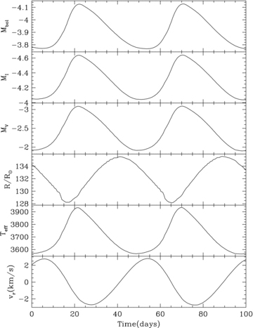
Mbol, MI, MV, R/R⊙, Teff and vr plotted against time in a model red giant variable pulsating in the first overtone mode. The radius R is defined at optical depth 2/3 and vr is the radial velocity seen by a distant observer. It is defined as −v/1.4, where v is the pulsation velocity, relative to the centre of the star, of matter near optical depth 2/3. The factor of 1.4 is the correction factor from observed to pulsation velocities for red giant pulsators (Scholz & Wood 2000).
The model shows that minimum light occurs between mean increasing radial velocity (as estimated here) and maximum radial velocity (as estimated by Lebzelter & Hinkle 2002). The model also predicts a ratio of velocity to I amplitude of 9.2 km s−1 mag−1, somewhat smaller than the estimate of 15 km s−1 mag−1 given here. Given the small size of the corrections to velocity that we have applied, the uncertainty in the relative phase and amplitude ratio of velocity and I amplitude will not significantly affect the resulting velocity curve of the sequence D variability.
2.5 Obtaining LSP parameters and narrowing the sample
Following the corrections described above, we were now in a position to analyse the light and velocity variations associated with the LSP. A binary fit was made to the corrected velocity data of the LSP using a fortran program, Fitall to obtain the parameters of the velocity curve. Fitall also made a Fourier series fit (with a frequency f and one harmonic 2f) to the MACHO MB, MR and OGLE I light curves, and to MB−MR. Some examples of the fits to the light and velocity data made by Fitall can be seen in Fig. 3. The complete set is available in the online version of this paper (see Supporting Information).
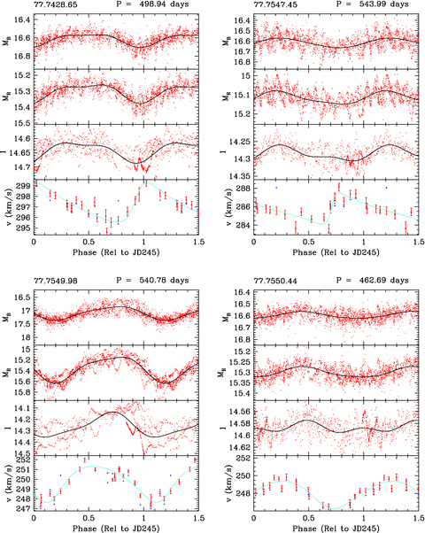
Light and velocity curves plotted against phase for four sequence D stars. The blue velocity points without error bars are the radial velocities without corrections and the red points with error bars are the radial velocities that have been corrected for pulsation and had specific date corrections. Also shown are the Fourier fits to the light data (black lines), and the binary fits to the velocity data (cyan lines), both made by Fitall. The complete set of fits is available in the online version of this paper (see Supporting Information).
Due to the poor quality of the data for some stars, the original sample of 58 sequence D stars had to be reduced. Some stars had large velocity errors due to poor quality or few spectra or no OGLE light curve, so they were excluded from the sample. A few stars had LSPs near 365 d leading to a large unfilled gap in the velocity curve, and could not be analysed.
Orbital elements.
| Star | γ(km s−1) | K (km s−1) | e | ω (°) | T (HJD) | P (d) | f(m) (10−4 M⊙) | No. obs. |
| 77.7427.41 | 239.812 ± 0.144 | 1.870 ± 0.175 | 0.436 ± 0.139 | 189.68 ± 6.91 | 3491.19 ± 13.82 | 776.18 | 3.835 ± 1.377 | 19 |
| 77.7427.72 | 273.087 ± 0.186 | 1.626 ± 0.271 | 0.547 ± 0.182 | 257.71 ± 6.59 | 3251.47 ± 10.27 | 488.67 | 1.277 ± 0.840 | 19 |
| 77.7428.65 | 297.159 ± 0.116 | 1.850 ± 0.095 | 0.402 ± 0.115 | 290.72 ± 4.53 | 3462.77 ± 4.97 | 498.94 | 2.512 ± 0.567 | 19 |
| 77.7429.100 | 313.955 ± 0.145 | 0.966 ± 0.188 | 0.187 ± 0.145 | 182.16 ± 12.49 | 3166.86 ± 16.46 | 473.24 | 0.419 ± 0.248 | 19 |
| 77.7429.47 | 280.326 ± 0.108 | 2.271 ± 0.120 | 0.475 ± 0.108 | 274.88 ± 3.59 | 3547.93 ± 9.50 | 1078.33 | 8.910 ± 2.264 | 19 |
| 77.7430.46 | 243.159 ± 0.129 | 1.687 ± 0.161 | 0.195 ± 0.127 | 279.99 ± 5.57 | 3370.88 ± 6.56 | 416.45 | 1.957 ± 0.579 | 19 |
| 77.7430.51 | 266.274 ± 0.212 | 2.203 ± 0.137 | 0.583 ± 0.202 | 227.13 ± 3.50 | 4148.37 ± 11.12 | 798.34 | 4.737 ± 2.686 | 18 |
| 77.7547.44 | 271.204 ± 0.148 | 2.150 ± 0.163 | 0.151 ± 0.147 | 87.27 ± 4.59 | 3314.19 ± 10.26 | 870.06 | 8.654 ± 2.053 | 19 |
| 77.7547.45 | 285.675 ± 0.142 | 1.697 ± 0.181 | 0.590 ± 0.141 | 278.00 ± 3.93 | 3106.62 ± 6.16 | 543.99 | 1.450 ± 0.725 | 19 |
| 77.7549.42 | 263.993 ± 0.146 | 1.758 ± 0.235 | 0.274 ± 0.144 | 225.45 ± 3.01 | 3668.10 ± 7.03 | 868.76 | 4.351 ± 1.832 | 18 |
| 77.7549.46 | 263.453 ± 0.188 | 1.542 ± 0.225 | 0.201 ± 0.186 | 242.52 ± 12.16 | 3169.49 ± 20.31 | 742.68 | 2.651 ± 1.201 | 19 |
| 77.7549.98 | 249.842 ± 0.123 | 1.848 ± 0.101 | 0.232 ± 0.123 | 210.85 ± 5.25 | 3336.64 ± 7.44 | 540.78 | 3.254 ± 0.609 | 19 |
| 77.7550.43 | 244.373 ± 0.170 | 1.743 ± 0.235 | 0.391 ± 0.169 | 255.86 ± 7.39 | 3371.03 ± 9.06 | 452.37 | 1.936 ± 0.906 | 18 |
| 77.7550.44 | 247.976 ± 0.085 | 1.536 ± 0.129 | 0.118 ± 0.085 | 146.30 ± 4.21 | 3540.15 ± 5.29 | 462.69 | 1.701 ± 0.432 | 19 |
| 77.7552.111 | 273.144 ± 0.157 | 1.800 ± 0.180 | 0.217 ± 0.156 | 169.75 ± 6.69 | 3433.09 ± 8.76 | 462.96 | 2.604 ± 0.828 | 19 |
| 77.7667.918 | 260.681 ± 0.171 | 2.846 ± 0.130 | 0.409 ± 0.166 | 192.60 ± 5.54 | 3182.52 ± 4.05 | 310.17 | 5.632 ± 1.576 | 19 |
| 77.7669.1027 | 268.918 ± 0.202 | 3.360 ± 0.174 | 0.351 ± 0.202 | 276.46 ± 5.69 | 3167.47 ± 3.76 | 266.77 | 8.608 ± 2.477 | 19 |
| 77.7669.1028 | 220.264 ± 0.125 | 1.574 ± 0.186 | 0.171 ± 0.125 | 182.39 ± 5.47 | 3220.97 ± 9.44 | 623.22 | 2.409 ± 0.868 | 19 |
| 77.7669.973 | 273.015 ± 0.131 | 2.378 ± 0.215 | 0.257 ± 0.125 | 328.59 ± 2.37 | 3193.90 ± 2.05 | 367.77 | 4.622 ± 1.340 | 19 |
| 77.7669.991 | 302.589 ± 0.094 | 1.271 ± 0.105 | 0.529 ± 0.090 | 191.96 ± 7.42 | 3091.45 ± 4.05 | 241.77 | 0.315 ± 0.100 | 19 |
| 77.7671.282 | 239.954 ± 0.116 | 1.398 ± 0.184 | 0.259 ± 0.114 | 47.28 ± 3.13 | 3624.34 ± 7.04 | 836.86 | 2.133 ± 0.866 | 20 |
| 77.7672.38 | 253.020 ± 0.166 | 2.103 ± 0.175 | 0.363 ± 0.166 | 258.54 ± 9.82 | 3200.71 ± 11.93 | 660.92 | 5.154 ± 1.676 | 19 |
| 77.7673.25 | 252.165 ± 0.144 | 2.764 ± 0.215 | 0.201 ± 0.143 | 217.94 ± 3.67 | 3248.27 ± 4.43 | 392.27 | 8.067 ± 2.019 | 19 |
| 77.7910.59 | 319.326 ± 0.157 | 1.729 ± 0.168 | 0.300 ± 0.156 | 282.05 ± 5.50 | 3181.29 ± 7.37 | 473.72 | 2.203 ± 0.725 | 18 |
| 77.7912.33 | 322.424 ± 0.164 | 1.480 ± 0.183 | 0.257 ± 0.162 | 247.00 ± 7.50 | 3111.40 ± 5.92 | 320.79 | 0.973 ± 0.383 | 19 |
| 77.7912.36 | 300.304 ± 0.115 | 1.548 ± 0.147 | 0.618 ± 0.112 | 255.40 ± 4.39 | 3145.92 ± 4.22 | 519.20 | 0.970 ± 0.428 | 19 |
| 77.7912.66 | 264.590 ± 0.111 | 1.458 ± 0.178 | 0.487 ± 0.110 | 55.66 ± 5.03 | 3136.40 ± 3.33 | 339.35 | 0.725 ± 0.307 | 19 |
| 77.7914.39 | 237.481 ± 0.112 | 1.760 ± 0.130 | 0.120 ± 0.112 | 246.58 ± 5.57 | 3421.15 ± 10.36 | 717.39 | 3.964 ± 0.895 | 19 |
| 77.8034.380 | 238.063 ± 0.253 | 2.140 ± 0.099 | 0.322 ± 0.229 | 207.27 ± 5.82 | 3265.28 ± 10.60 | 401.59 | 3.459 ± 0.981 | 19 |
| 77.8035.48 | 302.518 ± 0.142 | 1.853 ± 0.167 | 0.081 ± 0.141 | 110.90 ± 8.01 | 3186.59 ± 16.24 | 719.69 | 4.695 ± 1.281 | 19 |
3 RESULTS
In this section, we discuss some general results that are not model specific. Model specific results are presented in Section 4.
3.1 The true distribution of the velocity amplitude
The distribution of velocity amplitude is an important parameter for most models of the sequence D phenomenon.
A histogram of the velocity amplitudes of our sample is shown in Fig. 4, with the values separated into bins of width 0.5 km s−1. It is important to note that we use the full or peak-to-peak amplitude, as opposed to the semi-amplitude. These amplitudes are obtained from the binary orbit fits to the observed velocities. We find that the velocity amplitude is concentrated mainly between 2.5 and 5.0 km s−1, with the highest number of stars falling in the bin centred at 3.5 km s−1. The distribution has a median value of 3.53 km s−1. Thus, our sequence D stars all have low, relatively similar velocity amplitudes. These results are consistent with the results of Hinkle et al. (2002)'s and Wood et al. (2004)'s analysis of Galactic LSP variables.
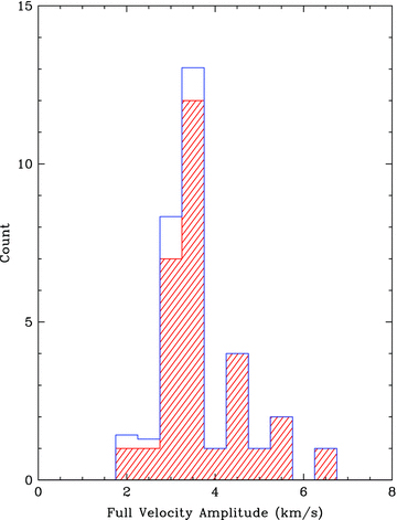
A histogram of the observed full velocity amplitude is plotted in red (forward shading). Note the clustering around 3.5 km s−1. Overplotted in blue is the modified histogram to account for the observational detection probability calculated in our Monte Carlo simulation (see text for details).
There are very few stars in our sample with velocity amplitudes <3.0 km s−1. To find out if we could detect such stars we performed a Monte Carlo simulation. 50 stars were simulated for each of the velocity amplitudes of 3.0, 2.0, 1.0 and 0.5 km s−1. The period, eccentricity and time of periastron were all selected randomly. The number of velocity points in each simulation was the same as the number of observations (19) and they were distributed in time identically to the observations. Random noise was added to each point, drawn from a normal distribution whose mean was the mean velocity error in the observations. In plots for visual examination, an error bar was added for each point, drawn from a uniform distribution between 0.2 and 0.5 km s−1 (consistent with observed errors).
A binary fit was made to the simulated velocities in the same way as to the observed velocities (see Section 2.5). The simulated data were put through the same reduction steps as the observed data, to see what percentage would pass. The percentages can be seen in Fig. 5. This tells us that we should be able to detect velocity amplitudes <3.0 km s−1. Using our simulated percentages, we can estimate the true number of stars at each velocity amplitude by dividing the observed histogram by the observable percentage. The resulting modified velocity amplitude histogram is shown overplotted on the observed histogram in Fig. 4.
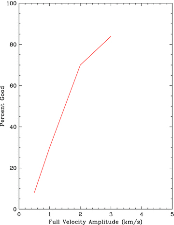
Fraction of simulated velocity curves which pass our data reduction process, for different velocity amplitudes.
The fact that we do not observe many sequence D stars with velocity amplitudes <3.0 km s−1 suggests that there are not many to be observed. We conclude that the true distribution of sequence D velocity amplitudes, represented in Fig. 4, shows a strong peak near 3.5 km s−1.
3.2 Correlation of light and velocity amplitudes
Light amplitude is plotted against velocity amplitude in Fig. 6. There is no obvious correlation between light and velocity amplitudes in either MB, MR or I. As noted previously the velocity amplitude has a small spread, and peaks at the small value of 3.5 km s−1. In particular, stars with small light amplitudes have velocity amplitudes as large as those stars with the largest light amplitudes.
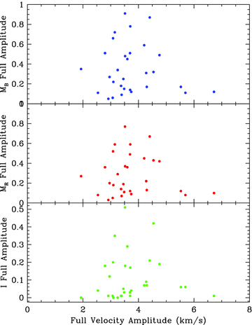
Light amplitude plotted against velocity amplitude for MB, MR and I.
3.3 Correlation of velocity amplitude with magnitude and period
Velocity amplitude is plotted against K magnitude in Fig. 7, which shows a suggestion that velocity amplitude increases slowly with luminosity. A similar correlation is seen in Fig. 8 between velocity amplitude and LSP. However, these possible correlations are disrupted by the presence of a few stars with larger velocity amplitudes, that fall apart from the general relation.
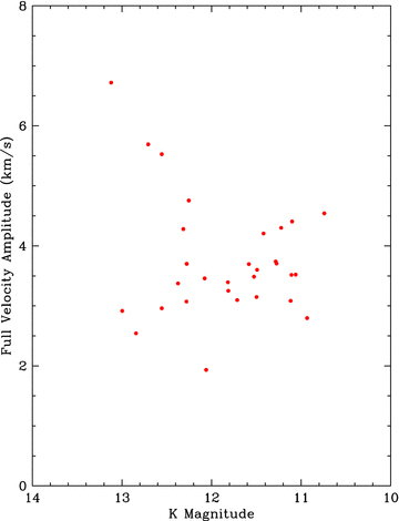
Velocity amplitude plotted against K magnitude.
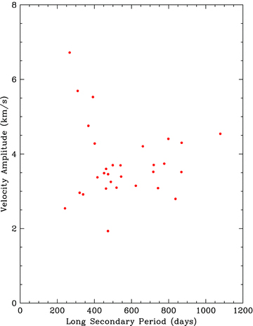
Velocity amplitude plotted against LSP.
4 TESTING AND CONSTRAINING MODELS
Here, we examine some of the more plausible and popular models of LSPs, in the light of our new data.
4.1 The binary model
The model of binary motion as an explanation for LSPs has been much debated since its proposal by Wood et al. (1999). In its favour, binary motion may be able to explain the sequence D velocity curves, and the light variation was originally thought by Wood et al. to resemble an eclipse of the star by a dusty cloud surrounding a small, orbiting companion. However, when this model was further examined by Hinkle et al. (2002) and Wood et al. (2004), two main problems were found: the companion mass was calculated to be always ∼0.1 M⊙, and the characteristic shape of sequence D stars' velocity curves was shown to imply that the angle of periastron is not uniformly distributed between 0 and 2π. With our larger sample we can place tighter constraints on these properties.
4.1.1 The companion mass
In a binary system, the velocity amplitude and period give an estimate of the mass of the companion. For a typical sequence D star with an LSP of 500 d, a typical velocity amplitude of 3.5 km s−1, and an assumed total system mass of M= 1.5 M⊙, the orbital separation is of the order of 1.4 au and the companion has a mass of 0.09 M⊙. This means it is a very low mass main-sequence star or a brown dwarf. There is an observed deficit of brown dwarf companions to main-sequence stars, compared to both more massive stellar companions and less massive planetary companions. This is known as the ‘brown dwarf desert’ (McCarthy & Zuckerman 2004; Grether & Lineweaver 2006). The range of likely companion masses can be found by calculating the companion mass for velocity amplitudes within 1σ of the mean of 3.5 km s−1. We find a companion mass range of 0.06 to 0.12 M⊙. Using the fits to the data in fig. 8 of Grether & Lineweaver (2006), we find that only 0.86 per cent of low-mass main-sequence stars have companions with masses in this range. Thus, binarity is an unlikely model, when we remember that ∼30 per cent of low-mass stars will exhibit LSPs when they pass through the AGB stage.
4.1.2 Correlation of velocity amplitude with light amplitude, magnitude and period
We would not expect the velocity and light amplitudes to be related in a binary model where the light variation is due to an eclipse phenomenon (by a cloud in the Wood et al. 1999 model). However, these amplitudes may be related if the light variations were caused by distortion of the red giant by its unseen companion (see Section 4.1.5).
As noted in Section 3.3, only a hint of a correlation is seen between velocity amplitude and K magnitude (Fig. 7), and with LSP (Fig. 8). We cannot draw any conclusions from this in the context of a binary model.
4.1.3 The distribution of the angle of periastron
One of the most conclusive ways to test the plausibility of the binary model as a cause for the LSPs is to examine the distribution of the angle of periastron, ω. As Hinkle et al. (2002) and Wood et al. (2004) note, the observed distribution of ω should be uniform over the whole range of angles, since one would expect binary orbits to be randomly aligned in space.
The angle of periastron was calculated by the program Fitall as part of the binary fit made to our radial velocity data. The distribution of the angle of periastron is plotted as a histogram in Fig. 9, with the data divided into bins 20° in width. Note that since the errors in the angle of periastron are typically around 5° (Table 2), the distribution of angle of periastron shown in Fig. 9 will not be significantly broadened by these errors. There is a clear bias in the distribution towards angles >180°, and the median of the sample is 227°. The distribution of the angles of periastron calculated by Hinkle et al. (2002) and Wood et al. (2004) for their small samples of Galactic stars has been overplotted. It is clear that their values of ω lie in the same region as the bulk of the present sample. This shows that the LSPs share a common cause, whether found in the LMC or in our own Galaxy.
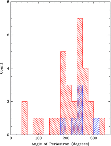
The distribution of the angle of periastron, ω. This study's sample is plotted in red (forward shading). The combined sample of Hinkle et al. (2002) and Wood et al. (2004) is shown in blue (back shading). Two stars have been dropped from Hinkle et al.'s sample and one from Wood et al.'s, due to overly large errors for ω.
Hinkle et al. (2002) and Wood et al. (2004) both found that the characteristic shape of the velocity curves suggests an eccentric orbit and a large angle of periastron, and that the distribution of the calculated angle of periastron was inconsistent with what would be expected if the sequence D stars were binaries, as no satisfactory explanation could be found for this bias towards higher angles. But given their small sample size, their conclusions were not highly significant. We can quantify and greatly improve these claims by using a Kolmogorov–Smirnov, or K–S Test, with our new data.
We have used the one-sample K–S Test, in the form of the fortran 77 subroutine ksone (provided in Press et al. 1986), to compare our distribution of the angle of periastron to the uniform distribution. We find that the probability that our distribution of ω is consistent with the uniform distribution is 1.4 × 10⁻³. In other words, the probability that the sequence D stars are binaries is extremely small. This is a major result from this study.
An angle of periastron between 180° and 360° means that at periastron, the red giant is closest to the observer, with the smaller companion further away. It is hard to see what selection effects could cause an LSP to be observed only in these binary orientations.
4.1.4 The distribution of the eccentricity
A histogram showing the distribution of the eccentricity is shown in Fig. 10. The eccentricity was calculated by Fitall as one of the orbital parameters of the binary fit to the velocity data.
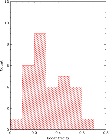
The distribution of the eccentricity.
The plot shows that if the sequence D stars are caused by binary motion, then they are in eccentric orbits. This confirms the suggestion of Hinkle et al. (2002) and Wood et al. (2004). The median eccentricity of the sample is 0.3.
4.1.5 Ellipsoidal variables
An ellipsoidal variable is a binary star which is tidally distorted by an orbiting companion into an ellipsoidal shape. Light variability is caused mostly by the variation of the apparent surface area of the star seen by the observer as the star rotates. Its velocity curve is dominated by orbital motion, with a small contribution from the rotation of the limb-darkened ellipsoid.
The light curve for an ellipsoidal variable is expected to have two maxima and minima per orbit, due to the star's shape. However, the velocity curve is expected to have only one maximum and minimum per orbit. We can use this characteristic to investigate the plausibility of ellipsoidal variability as an explanation for the LSP variation.
Soszyński et al. (2004b) show that the light curves of sequence E variables are satisfactorily explained by ellipsoidal variability. Their data show a partial overlap of sequences D and E in the period-luminosity diagram, and so they suggest that the LSPs may have a binary ellipsoidal origin. Soszyński (2007) explores this possibility further by searching for ellipsoidal or eclipsing shapes in residual LSP light curves. He finds these variations in ∼5 per cent of his sample, and adopts the binary model to explain LSPs.
However, with our new data set (which includes some sequence E stars), the difference between sequence D and sequence E mechanisms can now be vividly demonstrated by the difference between the light and velocity curves of sequence D and E stars. The phased-up light and velocity curves of sequence E stars show that the light curve completes two full cycles to every single cycle of the radial velocity, as expected for an ellipsoidal variable (Adams, Wood & Cioni 2006; Nicholls, Wood & Cioni, in preparation). However, Fig. 3 shows that sequence D stars do not display this behaviour: the phased-up light and velocity curves match each other cycle for cycle. Furthermore, sequence E stars typically have velocity amplitudes of 30 km s−1 or more while the sequence D stars have significantly lower typical amplitudes of 3.5 km s−1. Soszyński (2007) predicted that sequence D stars showing residual ellipsoidal or eclipsing-type variations should have large velocity amplitudes, similar to those observed for sequence E stars. One of our stars (77.7671.282) was noted by Soszyński as a double-humped LSPV and its velocity amplitude is only ∼4 km s−1. Additionally, none of our LSP sample shows typical sequence E velocity amplitudes (see Fig. 4). Sequences D and E variables clearly have distinctly different velocity amplitudes.
There is an unambiguous distinction between the mechanisms of variability responsible for causing sequences D and E. We can now state with some certainty that binary star ellipsoidal variability is not the cause of the LSP.
Similar to the sequence E ellipsoidal variables are symbiotic binaries, which are red giants with an accreting white dwarf companion, often in an eccentric orbit. Radial velocity amplitudes of these systems are usually ≥8 km s−1, and the red giant may be a Mira variable (Hinkle et al. 2006). However, symbiotic spectra show high temperature emission lines from accretion on to the white dwarf, something that has not been seen in either the sequence E or sequence D spectra. There does not seem to be any relation between the symbiotic stars and the sequence D stars.
4.2 Radial pulsation
There are several ways in which the present data set can be used to test radial pulsation models.
4.2.1 The phase difference between light and velocity curves
Minimum light and the mean of the velocity during its increase are relatively well defined for our sequence D stars. In order to examine their relative phases, a histogram of the phase difference between minimum light and mean rising velocity is shown in Fig. 11. The phases of minimum light and mean rising velocity were obtained from the fits made to the light and velocity curves. Each panel shows a strong peak of phase differences lying between 0 and 0.2 and there is little spread in phase.
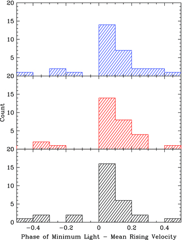
Histograms of the difference between the phase of LSP minimum light and the phase of mean rising LSP radial velocity. The top panel shows the phase difference for MACHO MB, the middle panel MR and the bottom panel OGLE I. Radial velocity is defined with respect to the observer: a positive radial velocity corresponds to matter moving away from the observer, that is, infalling to the centre of the star in a radial pulsation model.
Lebzelter et al. (2000) and Lebzelter & Hinkle (2002) find that for radially pulsating SRVs, the light lags the radial velocity by roughly 0.5 in phase, which means that minimum light occurs ∼0.25 in phase after the time of mean rising velocity. Our model SRV (Fig. 2) shows that minimum light occurs close to 0.23 in phase after mean rising velocity. Our sequence D stars are significantly different. Taking the main peak of light-velocity phase differences in Fig. 11 (values between −0.1 and 0.3), the mean phase shift is 0.1, and the standard deviation is 0.08. More simply, minimum light usually occurs ∼0.1 in phase after mean rising velocity. Radial pulsation therefore may not be consistent with this aspect of the LSP phenomenon, although this is not a strong conclusion.
4.2.2 The shape of the velocity curve
During large amplitude radial stellar pulsation (as in Mira variables), a shock wave from the interior of the star causes the surface layers to rapidly accelerate outwards, and then settle back more slowly. This is also shown in the shape of the velocity curve of our low amplitude model SRV, Fig. 2. The velocity curves of most of our sequence D stars show exactly the opposite of this behaviour: typically, we find a rapid increase in radial velocity with a correspondingly slower decline (see Fig. 3). In a radial pulsation model, this translates to a slow increase in stellar radius and a quick decrease. This has not been observed in any red giant stars known to be radially pulsating variables (e.g. Hinkle, Scharlach & Hall 1984; Lebzelter 1999, for Mira variables and SR variables, respectively).
4.2.3 Correlation of velocity amplitude with light amplitude, magnitude and period
The lack of correlation between velocity amplitude and light amplitude for the stars in our sample (see Fig. 6) is an unexpected result for pulsation mechanisms as they would be expected to show a positive correlation between light and velocity amplitude (Hinkle, Lebzelter & Scharlach 1997). Additionally, correlations of velocity amplitude with luminosity and with period are expected for radially pulsating variables. However, Figs 7 and 8 show that any correlations between these quantities in our sample are vague at the best. We are unable to draw any conclusion from this in the context of radial pulsation.
4.2.4 The variation of stellar radius
The stellar radius can be calculated from our data in several ways. Our first method was to calculate R using the Stefan–Boltzmann equation L= 4πR2σT4eff, with L and Teff calculated from MACHO photometry (see Appendix).
Examples of the variation of stellar radius calculated from the photometry, Rphot, can be seen in Fig. 12. There is generally a clear periodic curve at the period of the LSP as well as a scatter due to the primary pulsation. Plots for the entire sample are available in the online version of this paper (see Supporting Information).
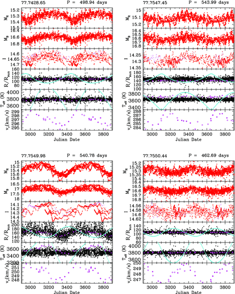
Different properties of four typical sequence D stars plotted against Julian Date. Solid symbols denote values plotted at the date of measurement while open symbols are values that have been shifted forward or backward by one or more periods. Top panel: MACHO red light curve. Second panel: MACHO blue light curve. Third panel: OGLE I light curve. Fourth panel: variation of Rphot (small black points), variation of Rvel (cyan curve) and variation of Rspec (large magenta points). Fifth panel: variation of Teff(phot) (small black points), variation of Teff(spec) (large magenta points) and variation of Teff(vel) (cyan curve). Bottom panel: observed radial velocity. See text for details. Plots for the entire sample are available in the online version of the paper (see Supporting Information).
Variation of stellar radius can also be calculated from the velocity, using  where v is the fit to the velocity data made by Fitall. If we assume that the velocity changes are due to radial pulsation, then this gives the expected radius variation for radial pulsation, Rvel, where the resulting radius has been normalized to the median photometric radius. Here, the velocity fit data were scaled by a factor of 1.4 to convert from observed to true pulsation velocity in red giants (Scholz & Wood 2000; Wood et al. 2004). The radius change computed from the velocity fit is shown in Fig. 12. Again it shows a clear periodic curve.
It is also possible to calculate stellar radius from the Stefan–Boltzmann equation using an effective temperature derived from the spectra, as opposed to the photometry (spectral Teff derivation is described in Section 4.2.5). The luminosities at the times of the spectra were in this case calculated from the fits to MB, MR and MB−MR as described in the Appendix. The radius calculated in this manner, Rspec, can also be seen in Fig. 12.
A histogram comparing the median values of Rphot and Rspec is shown in Fig. 13. For both radius estimates, most stars have median radii lying between 100 and 200 R⊙. The median values for the entire sample for Rphot and Rspec are 135.4 and 132.1 R⊙. Rvel is not shown, as it is normalized to Rphot.
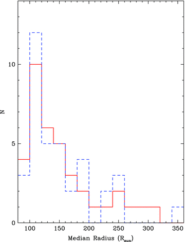
Distribution of median values of Rphot (solid red line) and Rspec (dashed blue line).
The radial amplitudes of our stars mostly lie between 3 and 60 R⊙ for all three variations. The median amplitudes of the sample for ΔRphot, ΔRspec and ΔRvel are 5.92, 5.62 and 40.02 R⊙, respectively.
Fig. 14 shows the distribution of radial amplitude ΔR divided by period, P. This quantity is a more sensitive indicator of differences between stars and models than the amplitude itself. In a radially pulsating model, one would expect the amplitude, ΔR, to be tightly correlated to the period if the velocity amplitudes are the same i.e. ΔR/P would be a constant. Given that our stars show very similar velocity amplitudes (see Fig. 4), we should expect tight, and similar, peaks for all three radius variations.

Distribution of radial amplitude/period for Rphot (solid red line, forward shading), Rspec (dashed blue line) and Rvel (dot–dashed green line, back shading).
From Fig. 14, it is clear that the distributions of ΔRphot/P and ΔRspec/P, are similar, but they are not the same as for ΔRvel/P. ΔRvel is computed assuming radial pulsation. Given that it appears that the three radius variations do not agree, the assumption that ΔR is due to radial pulsation of the star is unlikely.
Fig. 15 shows the distribution of ΔR divided by R. For Rphot and Rspec, the fractional radius change is usually 10 per cent or less. For Rvel, the fractional radius change is much larger, usually between 10 and 50 per cent. Once again, the assumption that the measured radial velocity variations are due to radial pulsation does not seem to be correct.
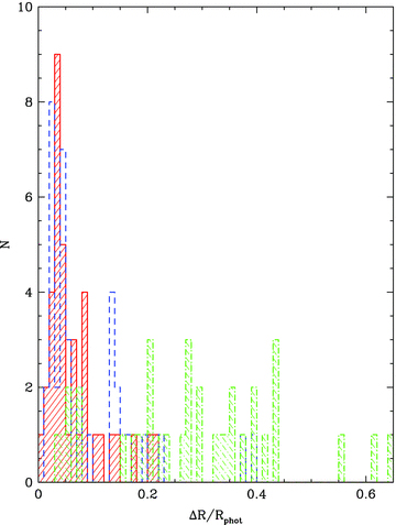
Distribution of relative radial amplitude for Rphot (solid red line, forward shading), Rspec (dashed blue line) and Rvel (dot–dashed green line, back shading).
A histogram comparing the phases of the three radius variations to the phase of the MR light curve is shown in Fig. 16. We compared the phase of minimum radius with the phase of minimum light, as these are both well-defined parts of the curves. In order to calculate these phases, a Fourier series with four terms was fit to the radius curves. For the light curve, the previously used Fourier fit was used (see Fig. 3). Fig. 16 shows that Rphot and Rspec both vary almost in phase with the light variation (phase differences generally ≤0.1). On the other hand, Rvel is more likely to be out of phase with the light (and consequently with the other radius variation estimates). Again, the assumption that the observed radius variations can be attributed to radial pulsation leads to inconsistencies.
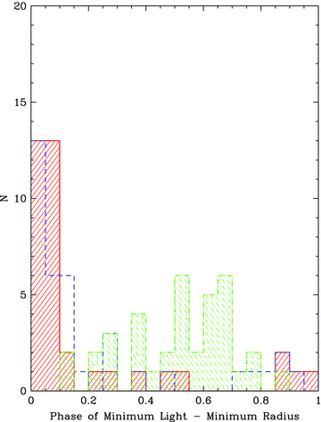
Distribution of phase of minimum light minus phase of minimum radius for Rphot (solid red line, forward shading), Rspec (dashed blue line) and Rvel (dot–dashed green line, back shading).
Using our model SRV (see Section 2.4), minimum radius occurs about 0.7 in phase before minimum light (Fig. 2). Of our variations, Rvel is the most similar to this. Rphot and Rspec, whose phases agree well with each other, do not show the radius–light phase relation expected for radial pulsation.
Overall, the discrepancy between the variations of Rvel and the other two radius estimates suggests that radial pulsation is unlikely to be the cause of the LSPs.
4.2.5 The variation of effective temperature
The variation of Teff was calculated from the photometry, from the spectra and from the velocity fit.
The variation in the photometric Teff(Teff(phot)), whose derivation is described in the Appendix, is shown in Fig. 12.
Teff was also calculated using the depth of the TiO bandhead at 7054 Å(Teff(spec)). The depth was calculated as the ratio of the mean count level of a 4 Å band longward of the bandhead to the mean count level of a 4 Å band shortward of the bandhead, taking into account the fact that the LMC has an average velocity of 270 km s−1, leading to a longwards wavelength shift of 6.3 Å in the spectra.
In order to calculate the effective temperature from the TiO depth, we calculated the depth of the TiO bandhead for nine Wing Spectral Standard stars. Then a quadratic fit was made to the TiO depth-spectral type data. This quadratic fit was used to calculate the spectral types of our sequence D stars from their TiO depths, and the effective temperatures were then calculated using the Ridgway et al. (1980)Teff–spectral type relation. An example of the typical variation of Teff(spec) in these stars can be seen in Fig. 12.
Some of the warmer sequence D stars in our sample showed little to no evidence of TiO in their spectra, and so we were unable to include these in the Teff(spec) calculation. However, good-quality velocity curves were not necessary for calculating Teff(spec) so a number of stars previously discounted from the velocity studies were added in where consideration of radius and effective temperature was required. Overall there was a net increase in sample size from 30 to 37 (the stars added in were excluded only from the velocity amplitude, angle of periastron, eccentricity and velocity phase parts of this work).
We also calculated the effective temperature variation expected for radial pulsation, Teff(vel). This was calculated from the radius change computed for pulsation in Section 4.2.4, the luminosity calculated from the fits to the photometry, and the Stefan–Boltzmann equation. The variation of Teff(vel) can be seen in Fig. 12.
The distributions of the median values for each star of Teff(phot) and Teff(spec) are shown in Fig. 17. Most stars have median effective temperatures lying between 3300 and 3800 K. The median values for the entire sample for Teff(phot) and Teff(spec) are 3662.9 and 3725.2 K. Teff(vel) is not shown, as it is calculated from Rvel, which is normalized to Rphot.

Distribution of median values of Teff(phot) (solid red line) and Teff(spec) (dashed blue line).
Fig. 18 shows the distribution of Teff amplitude for the three variations. The amplitude distributions of Teff(phot) and Teff(spec) are both strongly peaked at lower values, but ΔTeff(vel) shows a much wider distribution, and tends towards much larger amplitudes. The amplitudes of Teff(phot) and Teff(spec) mostly lie between 20 and 200 K, but Teff(vel) amplitudes tend to lie between 200 and 800 K. The median amplitudes of the sample are 42.3, 72.56 and 582.78 K for ΔTeff(phot), ΔTeff(spec) and ΔTeff(vel), respectively. Teff(vel), like Teff(phot), is a predicted temperature, whereas Teff(spec) is measured from our data. Teff(vel) has very large amplitudes in the context of radial pulsation. Adding this to the fact that Teff(vel) does not agree with Teff(spec) suggests that radial pulsation cannot explain the LSPs.
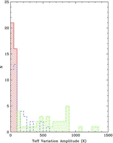
Distribution of amplitude of effective temperature variation for Teff(phot) (solid red line, forward shading), Teff(spec) (dashed blue line) and Teff(vel) (dot–dashed green line, back shading). The higher end of the ΔTeff(vel) distribution has been cut off, in order to show greater detail at the peaks of ΔTeff(phot) and ΔTeff(spec).
Fig. 19 shows the relation of light amplitude to Teff amplitude for both Teff(phot) and Teff(spec). The graph shows that Teff amplitude increases with increasing MR amplitude, for both Teff(phot) and Teff(spec).
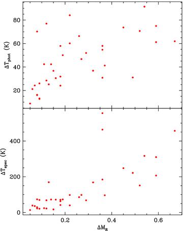
Top Panel: ΔTeff(phot) plotted against ΔMR. Bottom Panel: ΔTeff(spec) plotted against ΔMR.
5 DISCUSSION AND CONCLUSIONS
5.1 The movement of the visible surface of a sequence D star during its LSP
Possibly the most remarkable feature of the sequence D stars is the large change in the radial distance to the visible surface of a sequence D star as it passes through one LSP. By integrating the radial velocity with time, we calculated in Section 4.2 a radius change for radial pulsation between 3 and 60 R⊙, with the typical radius full amplitude being ∼41 R⊙. The typical median radius of a sequence D star is around 135 R⊙.
We can use this property to demonstrate just how unlikely radial pulsation is in these stars. An amplitude of 41 R⊙ in a 135 R⊙ radially pulsating star corresponds to a fractional radius change of over 30 per cent from minimum to maximum radius. These radial amplitudes are very large in the context of radial pulsation: fundamental-mode Mira variables pulsate with radius changes of the order of 50 R⊙ (Ireland, Scholz & Wood 2004), but they have visible light amplitudes of ∼6 mag, while typical sequence D stars have light amplitudes of ΔMR≤ 0.8 mag. It seems unlikely that such a modest light change could be associated with so large a radius change, suggesting that radial pulsation is not the cause of LSPs.
This comparative analysis backs up a huge problem with the radial pulsation model which was raised in section 4.2: the changes in radius would lead to changes in Teff that are vastly greater than the directly observed changes from spectra or photometric colour.
In addition to the problems with radial pulsation raised by our own data, there are also other problems raised by Wood et al. (2004): the length of the primary period does not vary during the LSP as expected; and to date there is no known mode of radial pulsation that has the required periods.
Wood et al. (2004) proposed non-radial pulsation as a possible cause for the LSPs. They showed that the best match to the observed periods is given by the g mode with n= 2 and l= 2. In this case, the net apparent radial velocity arises from some parts of the visible surface approaching while other parts are receding. Thus at a given position on the stellar surface, the velocity amplitudes and overall radial motions will need to be even larger than in the radial pulsation case. Given the large amplitudes calculated in this work for radial pulsation, non-radial pulsation would lead to distortions of the star that appear far too large to be credible, especially since g modes have significant amplitudes only in radiative regions (Wood et al. 2004).
It would therefore seem that the only way to generate the observed change in radial distance to the visible surface of a sequence D star is to have the star itself move, i.e. it must be in a binary system. Binary models, however, are inconsistent with various observational results described above. Most particularly, the non-uniform distribution of the angle of periastron and the low companion masses of these stars appear incompatible with a binary system model. The problem of the companion mass might be overcome if the companions were initially planets in eccentric orbits whose mass has been increased via accretion of material from the red giant. This would mean that although the companions currently have masses in the Brown Dwarf range, they were not born as Brown Dwarfs. To remove the problem of the non-uniform distribution of angle of periastron, we would need to have an observational selection effect that rejects angles of periastron in the range 0°–180°, i.e. we would need an effect that masks the sequence D variation when periastron occurs with the smaller companion in front of the red giant. An effect which could produce this bias is difficult to imagine.
5.2 Attributes of the Long Secondary Period
As with past studies, we are unable to find definitive evidence for any model which explains the LSPs in sequence D stars. To conclude, we therefore list all the currently known properties of LSPs. Any proposed model for LSPs should be able to explain all of these attributes.
Stars exhibiting LSPs occupy a clearly defined period-luminosity sequence.
LSPs are of length ∼250–1400 d.
LSP light variation is not regular and minima, in particular, vary in depth from cycle to cycle (see fig. 2 of Wood et al. 1999).
The primary pulsation is visible in the light curve at all times throughout the LSP and the primary period does not significantly change with LSP phase (Wood et al. 2004).
The ratio of LSP to pulsation period is ∼8–10. The shorter period variation lies usually on sequence B and is thought to be the first or second overtone radial pulsation (Wood et al. 1999; Ita et al. 2004; Fraser et al. 2005).
Lack of spectroscopic line broadening in observations of sequence D variables indicates that any rotational velocities are ≤3 km s−1 (Olivier & Wood 2003).
The radial velocity curves show a characteristic shape: observed radial velocity increases quicker than it decreases.
The velocity amplitudes cluster tightly around 3.5 km s−1.
The light–velocity phase shift for both the short period and the LSP is ∼0.25, with the light lagging the velocity. Minimum light is roughly aligned with mean rising velocity.
The ratio of colour to light variation of the LSP and primary oscillations are similar (Wood et al. 2004). Similarly, Derekas et al. (2006) showed that the ratio of blue to red amplitude of the LSP was similar to the ratio for stellar pulsation, and somewhat different from that due to ellipsoidal light variations.
There is no correlation between LSP light and velocity amplitude.
Stellar radius tends to be between 100 and 200 R⊙, with large radius variations of 3–60 R⊙ (if it is assumed that the LSP is caused by radial pulsation).
The equivalent width of the Hα absorption line varies with the LSP, indicating chromospheric activity (Wood et al. 2004).
PRW has been partially supported in this work by the Australian Research Council's Discovery Projects funding scheme (project number DP0663447). We are grateful for the multiple allocations of VLT service time over several semesters for this extended series of observations (program identifiers 072.D-0387, 074.D-0098, 075.D-0090 and 076.D-0162). This paper utilizes public domain data obtained by the MACHO Project, jointly funded by the US Department of Energy through the University of California, Lawrence Livermore National Laboratory under contract No. W-7405-Eng-48, by the National Science Foundation through the Center for Particle Astrophysics of the University of California under cooperative agreement AST-8809616, and by the Mount Stromlo and Siding Spring Observatory, part of the Australian National University.
REFERENCES
Appendix
APPENDIX A: CALCULATING LUMINOSITY AND EFFECTIVE TEMPERATURE FROM PHOTOMETRY
The luminosity was calculated from the MACHO Red photometry. The MACHO red and blue magnitudes were first dereddened using a colour excess of E(B−V) = 0.08 for the LMC (Keller & Wood 2006) and absorption A(λ) calculated by the reddening law from Cardelli, Clayton & Mathis (1989). This gave A(MB) = 0.2531 and A(MR) = 0.1783.
 (where the zero subscript denotes dereddened values) was derived through the following process. Note that we excluded the carbon stars in this procedure since the standard relations do not apply to them. First, the bolometric correction to V0 was calculated, using a calibration derived from the data of Fluks et al. (1994),
 was calculated from
 , it was a simple step to calculate
  using
using 
Supporting Information
Table 1. Heliocentric radial velocities and Julian dates for MACHO Sequence D stars.
Figure 3. Light and velocity curves plotted against phase for sequence D stars.
Figure 12. Different properties of sequence D stars plotted against Julian Date.
Please note: Wiley-Blackwell are not responsible for the content or functionality of any supporting materials supplied by the authors. Any queries (other than missing material) should be directed to the corresponding author for the article.
