Features of galactic halo in a brane world model and observational constraints Free

Abstract

1 INTRODUCTION

Early observations led to the hypothesis that there could be large amounts of non-luminous matter hidden in the galactic haloes (Oort 1930; Zwicky 1933, 1937). Later observations of flat rotation curves of spiral galaxies confirmed the hypothesis (Freeman 1970; Roberts & Rots 1973; Ostriker, Peebles & Yahill 1974; Einasto, Kaasik & Saar 1974; Rubin, Thonnard & Ford 1978; Rubin, Roberts & Ford 1979; Sofue & Rubin 2001; Kochanek et al. 2005). Doppler emissions from stable circular orbits of neutral hydrogen clouds in the halo allow the measurement of tangential velocity v_tg(r) of the clouds treated as probe particles. According to Newton's laws, centrifugal acceleration v²_tg/r should balance the gravitational attraction GM(r)/r², which immediately gives v²_tg=GM(r)/r. That is, one would expect a fall-off of v²_tg(r) with r. However, observations indicate that this is not the case: v_tg approximately levels off with r in the halo region. The only way to reconcile this result of observation is to hypothesize that the mass M(r) increases linearly with distance r. Luminous mass distribution in the galaxy does not follow this behaviour. Hence, we conclude that there must be huge amounts of non-luminous matter hidden in the halo. This unseen matter is given a technical name, dark matter. Gravitational lensing measurements have further confirmed the presence of dark matter (Maoz 1994; Barnes et al. 1999; Cheng & Krauss 1999; Sofue & Rubin 2001; Trott & Webster 2002; Weinberg & Kamionkowski 2002; Kochanek & Schechter 2004; Smith et al. 2005; Faber & Visser 2006; Metcalf & Silk 2007). Current estimates suggest that about 23 per cent of matter in the whole Universe consists of dark matter residing in the galactic haloes.

Although the exact nature of the dark matter is as yet unknown, several candidates for it have been proposed in the literature. One of the favoured candidates is the standard cold dark matter of the so-called SCDM paradigm (Efstathiou, Sutherland & Madox 1990; Pope et al., 2004). Despite its initial success, the current consensus seems to converge on the Lambda CDM or ΛCDM model that is related to the accelerating expansion of the Universe (Tegmark 2004a,b).

Analytic halo models include the framework provided by scalar–tensor theories. Scalar fields are important because they are predicted by supersymmetric unification theories (see e.g. Ellis et al. 1998). In particular, a prototype of scalar–tensor theories, namely the Brans–Dicke theory with scalar field φ, has the potentiality to explain a wide range of effects, from those in Solar system (Weinberg 1972; Bhadra, Sarkar & Nandi 2007) and gravitational lensing (Bhadra 2003; Nandi, Zhang & Zakharov 2006; Sarkar & Bhadra 2006) to those arising from objects as exotic as wormholes (Agnese & La Camera 1995; Nandi, Islam & Evans 1997; Nandi et al. 1998; Bhadra & Sarkar 2005). Fay (2004) considered a larger class of scalar–tensor theories with a potential V(φ), and with coupling parameter ω=ω(φ), for the investigation of galactic dynamics. Many other halo models including suitable variants of scalar field theories also exist in the literature (see e.g. Bekenstein & Milgrom 1984, Sanders 1984, 1986, Soleng 1995, Matos, Guzmán & Nuñez 2000, Peebles 2000; Nucamendi, Salgado & Sudarsky 2001, Mielke & Schunck 2002, Cabral-Rosetti et al. 2002, Lidsey, Matos & Ureña-Lopez 2002; Bharadwaj & Kar 2003; Arbey, Lesgourgues & Salati 2003). Substantial halo models are provided by the brane world theory (Mak & Harko 2004; Rahaman et al. 2008).

The motivation for the brane world model, which we are considering in this article, comes from an entirely different but important direction. It comes from the consideration of higher dimensional space–time because it can be argued that 4d is not big enough to fully accommodate the self-interaction dynamics of gravity. In a recent article, Dadhich (2009) has given persuasive arguments based on flat space imbedding, self-interaction and charge neutrality. But why only 5d and not higher? The reason is that the conformally flat Friedmann-Robertson-Walker (FRW) universe is embeddable only in 5d flat space–time, which means that free gravity does not propagate farther than 4d because the Weyl curvature vanishes for this FRW universe. The Randall & Sundrum (1999a,b) model provides the following setting: the three-brane (i.e. our 4d space–time which confines matter and other gauge fields) has zero Weyl curvature, and it bounds the 5d constant curvature bulk space–time. To probe into fifth dimension, one cannot rely on light signals as they do not propagate there. Therefore, a possible probe has to rely only on the propagation of gravity off the brane in an unfamiliar non-free manner (Dadhich 2009). For this, one needs to devise a purely gravity experiment and a method to fathom gravity propagation in higher dimension. This being a formidable task, the usual approach is to look for measurable imprints coming from 5d into known gravitational configurations. The galactic halo, where gravity is the king, provides a natural large-scale arena for this observation. It is quite probable that the effect of unseen dark matter is due to such imprints which contribute to the source term of Einstein's 4d field equations. Solving Einstein's equations, one then tries to work out the details of higher-dimensional non-local effects.

Static spherically symmetric exterior solutions of the brane world model have been derived in the literature (Dadhich et al. 2000; Germani & Maartens 2001; Casadio, Fabbri & Mazzacurati 2002; Visser & Wiltshire 2003; Harko & Mak 2004; Mak & Harko 2004; Creek et al. 2006; Viznyuk & Shtanov 2007). While all of these works are motivated by one or the other relevant considerations, the solution by Rahaman et al. (2008) is based on the simplest supposition of rotation curves that connects dark matter with the brane world model in a straightforward way. Whatever be the analytic model, there must be a way to contrast its predictions with actual measurements. The key point is that one does not directly measure the metric functions but indirectly measures gravitational potentials and masses from rotation curve and lensing observations. Bharadwaj & Kar (2003) advocated that a combination of rotation curves and lensing measurements could be used to determine the equation of state of the halo fluid, although their model was restricted to specific form of flat rotation curve as well as guesses on equations of state. Faber & Visser (2006) have shown how; in the first post-Newtonian approximation, the combined measurements of rotation curves and gravitational lensing allow inferences about the mass and pressure profile of the galactic halo as well as its equation of state.

In this paper, we wish to explore various features of the brane world solution by Rahaman et al. (2008) focusing in particular on the constraints imposed by combined measurements. Our general conclusion is that the model has a number of interesting properties. Nevertheless, it is too premature to say if the model is observationally supported. The relevant measurement constraints on the model are worked out. This paper is organized as follows. In this section, we have already delineated the motivation for the brane world model. In Section 2, we briefly outline the field equations and the solution under consideration for later use. Section 3 discusses the nature of the galactic fluid while Section 4 shows stability of circular orbits. In Section 5, we establish the attractive nature of gravity in the halo arguing from two different viewpoints, and in Section 6 we discuss observational constraints. In Section 7 we make a brief comparison with the central features of a scalar field model. Section 8 contains the conclusions.

2 FIELD EQUATIONS AND THE SOLUTION

The 5d bulk field equations with negative vacuum energy Λ₅ can be reduced to effective 4d gravitational field equations on the 3d brane. The governing equations are due to Shiromizu, Maeda & Sasaki (2000) which are

1

where the Roman indices run from 0 to 3, k²₅= 8πG₅ is the 5d gravitational constant, Λ is the 4d cosmological constant given by Λ=k²₅ (Λ₅+k²₅λ²_b/6), the 4d coupling constant k₄ is k²₄=k⁴₅λ_b/6 and λ_b is the vacuum energy on the brane. The stress E_ij is the non-local effect from the bulk given by (Dadhich et al. 2000)

2

where k=k₅/k₄, h_ij=g_ij+u_iu_j is the projection tensor, U=k⁴E_ijuⁱu^j is the so-called dark radiation energy density, Q_i is a spatial vector while P_ij is a spatial, trace-free symmetric tensor. The E_ij satisfies, in virtue of the Bianchi identities, the conservation law

3

where semicolon denotes covariant derivative with respect to g_ij. The simplest case is the case of vacuum (the absence of ordinary matter) so that T_ij= 0 ⇒S_ij= 0 which, in the paradigm of the study here, implies that we are interested in the region away from the galactic core, where the dark matter strongly dominates over the ordinary matter. In static vacuum, we have Q_i= 0 and in the comoving orthonormal frame, we have uⁱ=δⁱ₀, h_ij= diag (0, 1, 1, 1). In this case, the constraint equation (3) suggests a solution (Dadhich et al. 2000)

4

where r_i is a unit radial vector and P is the so-called dark pressure.

Let us consider a spherically symmetric line element

5

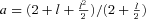
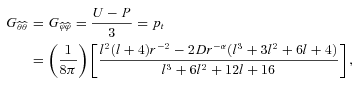
where ν and λ are the metric potentials and are function of the space coordinate r only, such that ν=ν(r) and λ=λ(r). For this symmetry, ⁠. In static vacuum (T_ij= 0, Q_i= 0) with the trace-free source term Eⁱ_i= 0 ⇒Rⁱ_i= 0, and with the unit radial vector r_i= (0, 1, 0, 0), the field equations (1) yield the following (Mak & Harko 2004):

6

7

8

9

where U=U(r), P=P(r) and primes denote differentiation with respect to r. Note that of Rahaman et al. (2008) has been properly rearranged in equation (8) above, which reveals the correct Ricci component on the left-hand side.

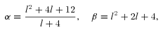
Assuming the known flat rotation curve condition constant (Chandrasekhar 1983), Rahaman et al. (2008) obtained a solution as follows:

10

11

where l= 2(v_tg)², B₀ > 0 and D are arbitrary constants and ⁠. They showed that the mass function increases linearly with r, which agrees with observation (Begeman 1989). However, this expression for mass is Newtonian and is applicable only so long as one can neglect pressure contributions although as yet there is no observational ground for such a neglect. To see the expressions for various types of mass distributions in terms of observational parameters, we wait till Section 6. Meanwhile, there are several other facets of the solution that need attention, which are addressed below.

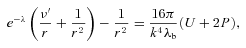
3 NATURE OF DARK RADIATION

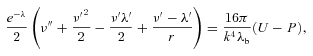
To throw some light on this issue, we identify the right-hand side of the equations (6)–(8) with the standard spherically symmetric fluid distribution (ρ, p_r, p_t, p_t) via Einstein's equations in the observer's orthonormal rest frame ⁠. Using equations (10) and (11) in (6)–(8), we get

12

13

14

15

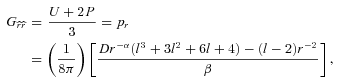
where we have chosen units on the right-hand side of equations (6)–(8) such that and redefined the fluid stresses (ρ, p_r, p_t, p_t) in terms of U and P. Eliminating U from equations (13), (14), one can easily find the expression for P(r) as given in Rahaman et al. (2008) after their arbitrary constant of integration is set to zero. There is actually no room for a non-zero constant because once the metric functions are known, U and P follow from equations (6)–(8).

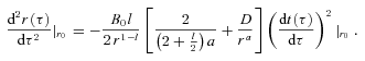
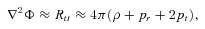
The interesting results we find are the following: while U is the same as ρ, the dark pressure P(r) is equal to neither p_r nor p_t but P(r) =p_r(r) −p_t(r) ≠ 0. This indicates that the dark Weyl radiation imprint cannot be characterized in the rest frame by a perfect fluid which requires p_r(r) =p_t(r). So the perfect fluid version of dark radiation is that U(r) ≠ 0 but P(r) = 0. Looking at equation (2), we see that the imprint radiation in 4d vacuum is a dust-like fluid where ⁠. This is not the case with the solution under consideration since p_r(r) ≠p_t(r). This pressure anisotropy is a good feature of the solution from the point of view of exterior matching. Note that the solution cannot be matched to the Schwarzschild exterior metric at the boundary of the halo if the pressures were isotropic (Bharadwaj & Kar 2003). The Schwarzschild solution, although not the unique spherically symmetric vacuum when considering the brane world model, is desirable for mimicking the far region (vacuum) of true 4d gravity, as supported by observation. We further see that the dark radiation fluid is not of exotic nature. The minimal condition for exoticity is that the Null Energy Condition (NEC) should be violated (Hochberg & Visser 1998). We find that the NEC is satisfied at all radii because ρ+p_r≥ 0 (Fig. 1). Transverse pressures are not included as they refer only to normal matter (Visser, Kar & Dadhich 2003). Even if we include them, we find ρ+p_r+ 2p_t≥ 0 for all r.

Figure 1

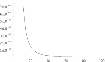
Plot of ρ+p_r with distance r in kpc. We find that ρ+p_r≥ 0 and that it rapidly decreases with distance, indicating that the pointwise NEC is satisfied. As mentioned in the text, in all the figures, the values of the constants are chosen as l= 0.000001 and D= 0.00001. The distances are shown along the abscissa.

Open in new tabDownload slide

In the rest of the article, we assume the following numerical values for constants. Observations of the frequency shifts in the H i radiation show that, in the halo region, v_tg/c is nearly constant at a value 7 × 10⁻⁴ (Binney & Tremaine 1987; Persic, Salucci & Stel 1996; Boriello & Salucci 2001). Thus l∼ 10⁻⁶. We also note that the solution is not used for small r, the inner core of the galaxy. Accordingly, to be consistent with observational facts, in all the figures in this paper we shall take B₀= 1, l= 0.000001, D= 0.00001 and fairly large distances in kpc.

4 STABILITY OF CIRCULAR ORBITS

Defining the four-velocity of a test particle moving solely in the subspace of the brane (and restricting ourselves to θ=π/2), the equation g_νσU^νU^σ=−m²₀ can be cast in a Newtonian form

16

which gives

17

18

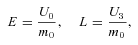
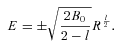
where the constants E and L, respectively, are the conserved relativistic energy and angular momentum per unit rest mass of the test particle. Circular orbits are defined by r=R= constant, so that and, additionally, ⁠. From these two conditions follow the conserved parameters:

19

and using it in V(R) =−E², we get

20

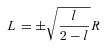
The orbits will be stable if and unstable if ⁠. Putting the expressions for L and E in ⁠, we obtain, after straightforward calculations, the final result, viz.,

21

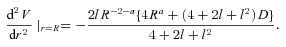
Thus so that circular orbits are stable in the model under consideration when D > 0. The latter condition is always satisfied since, from equation (11), we see that D has a dimension proportional to a power of radius R. The radius is always positive and so is D.

5 ATTRACTION IN DARK RADIATION

Now let us return to the question of attractive gravity. Observations indicate that gravity on the galactic scale is attractive (clustering, structure formation, etc.). By the existence of stable circular orbits we already know that the particles are being accelerated towards the Galactic Centre. This can also be seen by studying the geodesic equation for a test particle that has been ‘placed’ at some radius r₀, which yields

22

The quantity in square brackets is g^rr and must therefore be positive. Therefore, this expression is negative and it can be deduced that particles are attracted towards the centre. Detailed discussions on this quantity may be found in Ford & Roman (1996) and Lobo (2008). A related issue is the following. In the Newtonian limit, the gravitational energy of a spherically symmetric, gravitationally attractive system, with sufficient fall-off properties, is negative. One could potentially argue that the 4d gravitational effects due to higher dimensional Weyl stresses on the brane should not be subject to the same criteria as in true four-dimensional gravity. However, from the point of view of the Newtonian limit on the 3d brane, as well as CMB studies, it is desirable that the contribution from the Weyl stresses be not too large away from the galaxy. The question then becomes one of how to quantify such an effect in the relativistic case.

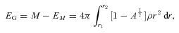
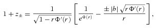
We choose as our quantifier the following: the total gravitational energy E_G in the halo region must be negative (Misner, Thorne & Wheeler 1973; Lynden-Bell, Katz & Bičák 2007), where by gravitational energy we mean the quantity defined below. It is necessary to explicitly verify it because a positive energy density does not always lead to attractive gravity (Nandi et al. 2009).

Hence we shall calculate the total gravitational energy E_G between two arbitrary but fixed radii with r > 0 (we have excluded the origin since the solution is not valid at small r because of singularity there, and the effects of the core region are manifest in the constants in the solution). This quantity is given by (Misner et al. 1973; Lynden-Bell et al. 2007)

23

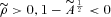
where by definition (proper radial length is larger than the Euclidean length) and

24

Here E_M is the sum of other forms of energy like rest energy, kinetic energy, internal energy, etc. The dark radiation energy density (12) can be rewritten as

25

For very small values of D and for 0 < l≪ 2, it follows from the integration in equation (24) that E_G < 0 for arbitrary r₂ > r₁ > 0, indicating that gravity in the halo is indeed attractive. It is observed that the galactic halo extends as far as 500 kpc (Sahni 2004). Thus, as an illustration we might take in units of kpc, r₁= 100, l= 10⁻⁶, then it follows from Fig. 2 that E_G < 0 for the upper limit r₂ < 500. We recommend a value of D≤ 0.00001 because it optimally yields reasonable behaviour for all relevant quantities in the entire range of the halo.

Figure 2

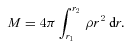
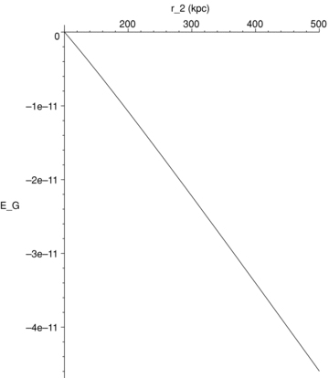
Plot of E_G(r₂) versus r₂. The lower limit of integration in equation (23) fixed at, say, r₁= 100 kpc while r₂ is varied from 100 to 500 Kpc. The value of E_G is very small but negative.

Open in new tabDownload slide

6 OBSERVATIONAL CONSTRAINTS

We wish to contrast the brane world model with the observational parameters in the galactic halo. For the ease of calculation, we shall rewrite the metric (5) in the form

26

where, for the solution under consideration, the metric functions are specifically given by

27

28

These functions are not necessarily the same as the potential and mass functions obtained from observations. Note from equation (28) that A > 1, which is a basic condition to be satisfied by a valid solution. In the first post-Newtonian approximation, the gravitational potential Φ(r) is given in general relativity by the equation (Misner et al. 1973)

29

which reduces to the equation for Newtonian Φ_N where

30

only if the pressure contributions are negligible in comparison to energy density.

The above general relativistic Φ appears in the wavelength shifts z_± of an emission line of a massive probe particle for an edge-on galaxy is (Nucamendi et al. 2001; Lake 2004)

31

where b is the impact parameter and ± signs refer to approaching and receding particles. The above equation (31) approximates to (Faber & Visser 2006)

32

Therefore, the usual techniques for obtaining the potential for rotation curve measurements yield a pseudo-potential

33

From equation (29), one then obtains a pseudo-mass as

34

The right-hand side expression comes from the first post-Newtonian order in the weak field limit, and we call it M_pN. We have so distinguished it because r²Φ′ (r) comes entirely from pseudo-potential Φ whereas M_pN is an integrated quantity that requires the knowledge of the equation of state. The pseudo-mass m_RC reduces to the Newtonian mass M(r) (see equation 24) when pressure contributions are negligible in comparison to energy density.

Photons can also be regarded as probe particles as they sense the gravitational field in the halo during their travel to the observer. The effect of gravity on photon motion can be calculated in terms of a refractive index n(r) (see also Boonserm et al. 2005). For the Schwarzschild gravity, the exact geodesic equation, including the equation for Shapiro time delay, of massless particles was expressed in terms of n(r) by Nandi & Islam (1995) via the idea of optical–mechanical analogy. This idea has been further extended by Evans et al. (2001) to arbitrary spherically symmetric space–times and by Alsing (1998) to rotating space–times. The geodesic motion of both massless and massive particles could be expressed exactly in terms of a single generalized refractive index N=n²V/c where V is the three-velocity of the particle. For light motion, V=c/n.

For unspecified metric functions Φ(r) and m(r), Faber & Visser (2006) argue that n(r) = 1 − 2Φ_lens+O[Φ²_lens] in which they define the lensing pseudo-potential as

35

Another pseudo-mass m_lens obtained from lensing measurements has been defined as (Faber & Visser 2006)

36

The first order approximations of Einstein's equations yield

37

38

where the right-hand sides denote, respectively, pseudo-density and pseudo-pressures. Furthermore, Faber & Visser (2006) defined a dimensionless quantity

39

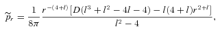
where the pseudo-quantities on the right-hand side of equations (37)–(39) determine, respectively, the observed density, pressure and equation of state. Using the specific metric functions (27, 28) in equations (35)–(39), we can calculate the first order quantities Φ_RC, m_RC, Φ_lens, m_lens, 2(m′_RC−m′_lens) and to be expected from combined observations.

Note that pseudo-quantities are the observable quantities. The general procedure to determine the metric can be stated as follows: once one is able to observationally determine the profiles of pseudo-quantities, one can work backwards to find the corresponding metric functions. This is a kind of reverse technique observational astrophysicists use. If the observed pseudo-profiles fit (up to experimental error) with the analytic profiles of a priori given metric functions, one can say that the solution is physically substantiated. Otherwise, it has to be ruled out as non-viable. In this sense, the observed pseudo-profiles play the role of constraints on the possible metric solutions.

For the present solution, we obtain the following constraint equations on Φ(r), m(r), the pressure profile and the equation of state:

40

41

42

43

44

45

with ⁠.

If observations yield the same profiles as on the right-hand sides, we can say that they support the metric functions Φ(r) and m(r) of equations (27, 28). Assuming for a moment that these specific functions are really observationally valid, we ask what comparative features of the observables do we expect to see. These can be visualized by first comparing the functions Φ_RC with Φ_lens. We plot their difference in Fig. 3 taking the numerical values of constants mentioned earlier and observe that despite their varying expressions, the actual difference Φ_RC−Φ_lens is negligible, of the order of only ∼10⁻⁶. Thus, rotation curve and lensing measurements lead to practically indistinguishable inferences about the pseudo-potential, at least in the first order. Similarly, Fig. 4 shows variation with distance of M_pN(r) and of different pseudo-masses m_RC and m_lens. All the masses share the common feature that they increase with distance r, though they begin to slightly differ in the far field. To ascertain the role of pressures from the observational standpoint, one has to look at Fig. 5 where we find that the difference m′_RC−m′_lens is of the order of ∼10⁻⁷, to first order. To ascertain the equation of state from observational parameters, we come to equation (44), which is plotted in Fig. 6. One immediately finds that ω→ 1/3. The closeness to 1/3 actually depends on the value of D, the smaller its value the better the closeness. The exact equation of state following directly from the equations (12)–(14) is

46

which implies from equation (39) that

47

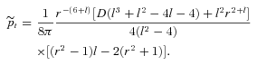
It is important to mention here that had the dark radiation been a perfect fluid, we could have ⁠, the usual equation of state for radiation. Noting that U=ρ and using equation (45) in equation (34) we find that the mass in the first post-Newtonian approximation becomes

48

which is twice the Newtonian mass M(r) defined by equation (24). All the above indicate that the galactic halo modelled by the present solution shows somewhat, but not quite, Newtonian features (pressure contribution is not negligible as it is proportional to energy density). The profiles of (pseudo) potentials, masses and the anisotropic equation of state as expressed in equations (40)–(44) above are the ones one would expect to find from the combined measurement of the pseudo-quantities, if the solution (27, 28) is really a viable one.

Figure 3

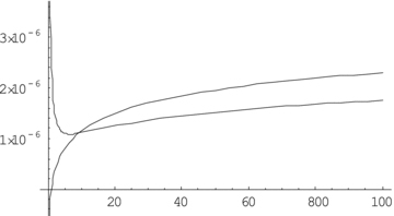
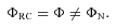
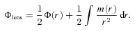
Upper curve represents the function Φ_lens and the lower curve Φ_RC. Although the functions differ nearer to the centre, the difference becomes only of the order of 10⁻⁶ as one moves away from the centre. Scalar field model provides the same behaviour.

Open in new tabDownload slide

Figure 4

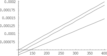
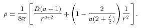
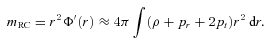
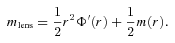
Upper line represents m_RC(r), the middle one m_lens(r) and the lower one M_pN(r). All the masses increase with distance, though they diverge in values in the far field because of varying pressure contributions.

Open in new tabDownload slide

Figure 5

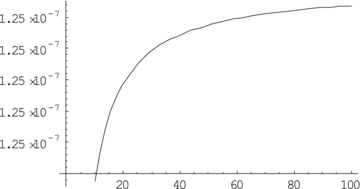
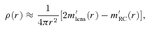
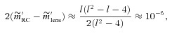
Plot of 2(m′_RC−m′_lens) versus r. We see that the numerical value of pressure is of the order of ∼10⁻⁷ like in the scalar field model. But this is of the same order as the energy density ρ (see equation 46), which indicates that pressure contributions are not altogether negligible in comparison to energy density. The solution thus can be said to describe a mild non-Newtonian system.

Open in new tabDownload slide

Figure 6

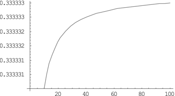
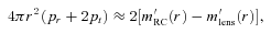
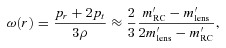
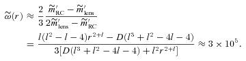
Plot of ω(r) versus r. We can clearly see that the equation of state predicted by the considered solution is ω= 1/3. One expects this radiation equation of state to be supported by combined observations. Scalar field model differs exactly here (see equation 61).

Open in new tabDownload slide

7 COMPARISON WITH A SCALAR FIELD MODEL

Scalar fields are an integral part of reality though they yet lack any observational evidence. We choose the well-discussed scalar field model with potential proposed by Matos et al. (2000) and compare it with the present brane world model. Using the flat rotation curve condition, they obtain the full solution as (we distinguish their quantities by tilde)

49

50

51

52

where D is an arbitrary constant of integration. For simplicity, they take D= 0, but this assumption makes (see equation 28). Because of this, their expressions for density and pressures lead to different conclusions than those in the brane world model considered here. For example, the expression for density exhibit ⁠, meaning violation of weak energy condition (WEC) and furthermore it leads to ⁠, implying repulsive gravity in the halo, which may not be as desirable as the attractive gravity scenario in the brane world model discussed here. Therefore, it is necessary to re-calculate the relevant quantities with D≠ 0.

We find the density and pressure profiles in the rest frame of the fluid as

53

54

55

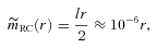
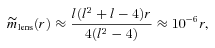
We wish to emphasize here that the role of non-zero value of D is crucial not only for avoiding repulsive gravity but also for arriving at a correct conclusion about the relative strengths between pressure and density. For instance, let us take D= 1. In the distant halo region, we can take, say, r∼ 100–300 kpc, and with l∼ 10⁻⁶, we find the numerical values to be and ⁠, which means that they are of the same order. But ⁠, which indicates that total pressure is roughly one hundred times less than the density. However, if we take D= 0.00001, we find that ⁠. If we keep on decreasing the value of D further (but never exactly to zero for reasons stated above), we see that the total pressure dominates more and more over density so that the system becomes indeed non-Newtonian as claimed by Matos, Guzmán & Nuñez (2000). Such minuscule values of D are remarkably similar to those recommended for our solution (see Section 5).

The next question is how far can we decrease D? We note the following interesting scenario: when D= 10⁻⁷, we find ⁠, which leads to ⁠. This is the extreme non-Newtonian model possible in the scalar field model. On the other hand, if D= 10⁻⁸, we find that up to r=r₀= 200 kpc (attractive gravity) and becomes after r=r₀ (repulsive gravity). At r=r₀, there is a singularity in ⁠. When D= 10⁻⁹, we find that ⁠, exhibiting the characteristics that follow from the same choice D= 0. Therefore, we conclude that the limiting value of D is 10⁻⁷.

The equation of state is anisotropic, as is evident from equations (54)–(55), a feature shared also by the brane world solution. It can be verified that for D≥ 10⁻⁷, so we can say that the halo matter is not exotic because the WEC and NEC are satisfied everywhere. Therefore, we expect an attractive halo. To confirm it, again we follow the prescription in Lynden-Bell et al. (2007), and find that the total gravitational energy is indeed negative:

56

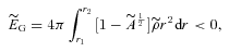
due to the fact that and r₂ > r₁.

Certainly, the extreme scalar field model corresponding to D= 10⁻⁷ is highly non-Newtonian, that is ⁠. As a result, equation (30) leading to a purely Newtonian definition of mass M(r) as in equation (24) does not apply. However, incorporating the pressure contribution, the dynamical mass in the first post-Newtonian order is

57

which clearly reflects the non-Newtonian nature of the model in terms of masses. The observable pseudo-quantities, for our chosen range r∼ 100–300 kpc, in this extreme case work out to

58

59

60

61

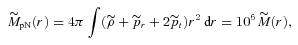
Note that if we straightaway put D= 0 in equation (61), we get ⁠, conveying a completely different conclusion. Thus, while the numerical values of observable potentials and masses behave like those in the brane solution, it is only the equation of state (61) that differs widely because has a value ∼10⁵ compared to (cf. equation 47). Therefore, we conclude that, with the suggested small non-zero values of D, the interesting model proposed by Matos et al. (2000) can also be a viable alternative.

8 CONCLUSIONS

In the foregoing, we first discussed the motivation for considering higher dimensions, which probably distinguishes the solution (27, 28) as a more interesting search for the halo model. It is the three-brane that we experience, and therefore the bulk contributions U and P are translated into brane quantities via Einstein equations, which provide a way to have insights into the nature of the galactic fluid. The present model shows that the halo does not have a perfect fluid equation of state but NEC is preserved, meaning that the fluid is not exotic. It was shown that circular orbits in the halo are stable and that the dark radiation is attractive in nature, as it must be. Thus, the solution satisfies two crucial physical requirements: circular orbit stability and attractive gravity in the halo. The next task was to derive the constraints on the solution imposed by combined observations of rotation curve and lensing.

The analyses by Nucamendi et al. (2001), Lake (2004) and Faber & Visser (2006) have been carried out without reference to any specific form of metric functions. The specific functions (27, 28) yielded the right-hand sides of equations (40)–(44) in terms of parameters to be measured by a combination of rotation curve and lensing measurements. These are effectively the constraint equations on the chosen solution. If combined observations turn out to tally with the behaviour predicted by equations (40)–(44), then the brane world solution (27, 28) can be said to be supported by observation. Until that happens, the solution would remain largely an academic curiosity.

As discussed in the Introduction, the increase of mass linearly with r comes from an elementary Newtonian argument to explain the observed fact of flat rotation curves. A key question still remains: how much of pressure contribution is there in the making of that mass; that is, is it just the Newtonian M(r) of equation (24) or M_pN(r) of equation (34)? The solution by Rahaman et al. (2008) does exhibit a linear increase of the Newtonian mass M(r). Fortunately, even if pressures are included, we find M_pN(r) = 2M(r) (cf. equation 48), that is they are of the same order showing that the theoretical linear mass increase is pretty consistent with both the definitions within the present model. Such an increase is also supported by observable pseudo-masses, as expected. However, this is just one aspect of the solution shared by many other models too. The distinguishing features lie elsewhere. For instance, we saw that in the scalar field model (cf. equation 57). As emphasized earlier, such distinguishing features will have to be determined only by the detailed analyses of data profiles of potential, pressure and, most importantly, the equation of state obtained through the combined rotation curve and lensing measurements. The bottom line is that the present solution depicts the halo as a mildly non-Newtonian model (pressure contribution is of the same order as energy density) in contrast to the highly non-Newtonian scalar field model. Although both the models share many properties including an anisotropic non-perfect fluid equation of state, sharp differences appear in the computation of M_pN(r) and in the equation of state characterized by ω(r). Observations to date do not seem yet conclusive enough (for a discussion, see Faber & Visser 2006) to tell us which one, if any, is closer to reality among all the competitive halo models.

We thank Arunava Bhadra for several enlightening discussions. KKN thanks Guzel N. Kutdusova for her assistance at BSPU and SSPA where part of the work was carried out.

REFERENCES