Jet and accretion power in the most powerful Fermi blazars Free

Abstract

1 INTRODUCTION

We would like to attack in a more systematic way than done in the past the problem of the relation between the power carried by the jet of blazars in the form of bulk motion of particles and magnetic fields, and of the luminosity associated to accretion. This task is not easy, mainly because of the Doppler enhancement of the non-thermal continuum produced by jets, and because this continuum very often hides the radiation produced by the accretion disc. However, starting from the early work of Rawlings & Saunders (1991), evidence has been accumulated that the jet power of extragalactic radio-loud sources is at least of the same order as the accretion one, and possibly a factor of ∼10 larger.

On the larger scale (radio-lobe size) one can resort to minimum energy considerations and estimates of the lifetime of radio lobes to find out the minimum jet power needed to sustain the radio-lobe emission (Rawlings & Saunders 1991). The main uncertainty associated to this argument is the unknown energy contained in the proton component.

At smaller, but still very large, jet scales (on kpc to Mpc), one can use the recently discovered (by the Chandra satellite) X-ray emission from resolved knots, to model it and to infer the total number of leptons needed to produce the observed radiation. Here the main uncertainties are related to the number of low-energy leptons (of energy γ_minm_ec² present in the source, a number that is rarely well constrained). Furthermore, one also needs to assume how many protons are associated for each emitting lepton. Assuming a one to one correspondence and using observed data to limit γ_min, Tavecchio et al. (2000, 2004, 2007), Celotti, Ghisellini & Chiaberge (2001) and Sambruna et al. (2006) derived jet powers that are comparable with those inferred at the subpc scales, suggesting that the jet powers in these sources are conserved all along the jet, with the caveat that for large-scale jets is difficult to constrain the bulk Lorentz factor Γ. However, values compatible with the inner jet are preferred (see Ghisellini & Celotti 2001).

A technique developed quite recently makes use of the cavities or ‘bubbles’ in the X-ray emitting intracluster medium of cluster of galaxies, and measures the energy required to inflate such bubbles. Assuming that this energy is furnished by the jet, one can calculate the associated jet power (i.e. Churazov et al. 2002; Allen et al. 2006; Balmaverde, Baldi & Capetti 2008).

At the Very Long Baseline Interferometry (VLBI) scale (pc or tens of pc), one takes advantage of the resolving power of VLBI to measure the size of the synchrotron emitting region: by requiring that the self-Compton process does not overproduce the total observed X-ray flux, one derives a lower limit to the Doppler factor δ[defined as δ= 1/[Γ(1 −β cos θ_v)], where θ_v is the viewing angle and Γ the bulk Lorentz factor], and a limit on the number of emitting particles and on the value of the magnetic field (Celotti & Fabian 1993). This in turn gives an estimate of the jet power. The main uncertainties here are the number of low-energy electrons (they emit unobservable self-absorbed synchrotron emission) and the fraction of the total X-ray flux produced by the radio VLBI knot.

The advent of the Compton Gamma-ray Observatory and its high-energy Energetic Gamma-ray Experiment Telescope (EGRET) instrument on one side, and of ground-based Cherenkov telescopes on the other, finally let it possible to discover at what frequencies blazar jets emit most of their power, i.e. above MeV energies. Variability of the high-energy flux also tells us that the emission site cannot be too distant from the black hole, while the absence of γ–γ absorption (leading to pair production) tells us that the emission site cannot be too close to the black hole and its accretion disc (Ghisellini & Madau 1996; Ghisellini & Tavecchio 2009; hereafter GT09). Bracketed by these two limits, one obtains a few hundreds of Schwarzschild radii as the preferred jet location where most of the dissipation occurs. Modelling the observed spectral energy distribution (SED) from the mm to the γ-ray band returns the particle number and the field strength needed to account for the observed data (see e.g. Maraschi & Tavecchio 2003; Celotti & Ghisellini 2008, hereafter CG08; Kataoka et al. 2008). Again, the main uncertainty in the game is γ_min, but in some cases γ_min can be strongly constrained. This occurs when the considered blazar has good soft X-ray data characterized by a flat spectrum. In these cases the X-ray emission is likely to be due to inverse Compton scatterings between low-energy electrons and seed photons produced externally to the jet (external Compton, EC; e.g. Sikora, Begelman & Rees 1994). In fact, while the synchrotron self-Compton (SSC) process uses relatively high-energy electrons and internal synchrotron radiation to produce X-rays, in the EC case we do see X-rays produced by electrons of very low energies, strongly constraining γ_min (see e.g. Tavecchio et al. 2007).

As for the accretion disc radiation, it is usually hidden by the stronger optical–ultraviolet (UV) synchrotron emission. However, in very powerful blazars we have good reasons to believe that the synchrotron component originating the radio to infrared (IR)–optical radiation is not completely hiding the thermal emission produced by the accretion disc. These reasons come partly from past observations of relatively high-redshifts blazars (even if not detected by Fermi or EGRET, see e.g. Sambruna et al. 2007; Landt et al. 2008; Maraschi et al. 2008, hereafter M08; GT09) and partly from theoretical considerations about the expected scaling of the magnetic energy density with the black hole mass: we expect lower magnetic fields in jets associated to larger black hole masses (e.g. GT09), and thus a reduced importance of the synchrotron component of the SED. Furthermore, the presence, in these objects, of broad emission lines of relatively ‘normal’ equivalent width (compared to radio-quiet objects) ensures that the thermal ionizing continuum cannot be much below the observed optical emission.

The above considerations guide us to select the most powerful blazars as very good candidates for measuring both the jet power and the accretion luminosity. In turn, since in these sources most of the luminosity is emitted in the hard X-rays and in the γ-ray band, it is natural to take advantage of the recently published list of blazars detected by the Large Area Telescope (LAT) on board the Fermi Gamma-ray Space Telescope (Fermi). It revealed more than 100 blazars with a significance larger than 10σ in the first 3 months of operation (Abdo et al. 2009a, hereafter A09). Of these, 57 are classified as flat spectrum radio quasars (FSRQs), 42 as BL Lac objects, while for five sources the classification is uncertain. Including two radio galaxies the total number of extragalactic sources amounts to 106. Redshifts are known for all FSRQs, for 30 BL Lacs, for one source of uncertain classification and for the two radio galaxies, for a total of 90 objects. Within this sources, there are 23 blazars exceeding an average γ-ray luminosity of 10⁴⁸ erg s⁻¹ within the 3-months survey. These are the targets of our study, aimed to estimate the power associated to accretion and to the jet. We will also take advantage of the optical–UV and X-ray observations made by the Swift satellite, to construct the SED of Fermi blazars, a crucial ingredient to reliably constrain the emission models leading to the jet and accretion power estimate.

In this paper we use a cosmology with h=Ω_Λ= 0.7 and Ω_M= 0.3, and use the notation Q=Q_X 10^X in cgs units (except for the black hole masses, measured in solar mass units).

2 THE SAMPLE

Table 1 lists 23 blazars taken from the A09 catalogue of Fermi detected blazars. We selected them simply on the basis of their K-corrected (see e.g. Ghisellini, Maraschi & Tavecchio 2009) γ-ray luminosity being larger than 10⁴⁸ erg s⁻¹. All sources but two are FSRQs. The exceptions are AO 0235+164 and PKS 0426−380, classified as BL Lac objects. However, these sources do have broad emission lines (see e.g. Raiteri et al. 2007 for AO 0235+164 and Sbarufatti et al. 2005 for PKS 0426−380), visible in low emission states. We therefore believe that AO 0235+164 and PKS 0426−380 are FSRQs whose line emission is often swamped by the enhanced non-thermal continuum. In Table 1 we mark the eight blazars for which there are public available Fermi light curves. Although we use for all blazars the 3-months averaged γ-ray flux and spectral index, for these eight sources we can check if at the time of the Swift observations the γ-ray integrated photon flux was much different than the average (the spectral index is available only for the 3-months average). For all sources but PKS 1502+106 we find a good consistency. For PKS 1502+106 the Swift observations were probably performed during the rapid decay phase after a major γ-ray flare. Therefore, it is difficult to assess the exact γ-ray flux during the Swift observation, but in any case it should not be different than the used average flux by more than a factor of 2.

3 SWIFT OBSERVATIONS AND ANALYSIS

For 17 of the 23 blazars in our sample there are Swift observations, with the majority of the objects observed during the 3 months of the Fermi survey. The data were analysed with the most recent software swift_rel3.2 released as part of the heasoft v. 6.6.2. The calibration data base is that updated to 2009 April 10. The X-ray Telescope (XRT) data were processed with the standard procedures (xrtpipeline v.0.12.2). We considered photon counting (PC) mode data with the standard 0–12 grade selection. Source events were extracted in a circular region of aperture ∼47 arcsec, and background was estimated in a same sized circular region far from the source. Ancillary response files were created through the xrtmkarf task. The channels with energies below 0.2 keV and above 10 keV were excluded from the fit and the spectra were rebinned in energy so to have at least 30 counts bin⁻¹. Each spectrum was analysed through xspec with an absorbed power law with a fixed Galactic column density from Kalberla et al. (2005). The computed errors represent the 90 per cent confidence interval on the spectral parameters. Table 2 reports the log of the observations and the results of the fitting the X-ray data with a simple power-law model.

Ultraviolet/Optical Telescope (UVOT; Roming et al. 2005) source counts were extracted from a circular region 5 arcsec sized centred on the source position, while the background was extracted from a larger circular nearby source-free region. Data were integrated with the uvotimsum task and then analysed by using the uvotsource task. The observed magnitudes have been dereddened according to the formulae by Cardelli, Clayton & Mathis (1989) and converted into fluxes by using standard formulae and zero-points from Poole et al. (2008). Table 3 lists the observed magnitudes in the six filters of UVOT, and the Galactic extinction appropriate for each source.

4 THE MODEL

To interpret the overall SED of our sources we use a relatively simple, one zone, homogeneous synchrotron and inverse Compton model, described in detail in GT09. This model aims at accounting in a simple yet accurate way the several contributions to the radiation energy density produced externally to the jet, and their dependence upon the distance of the emitting blob to the black hole. Here we summarize the main characteristics of the model. The emitting region, of size r_diss and moving with a bulk Lorentz factor Γ, is located at a distance R_diss from the black hole of mass M. The accretion disc emits a bolometric luminosity L_d. The jet is assumed to be accelerating in its inner parts, with Γ∝R^1/2 (R is the distance from the black hole), up to a value Γ_max. In the acceleration region the jet is assumed to be parabolic (following e.g. Vlahakis & Königl 2004); beyond this point the jet is conical with a semi-aperture angle ψ (assumed to be 0.1 for all sources).

The energy particle distribution N(γ)[cm⁻³] is calculated solving the continuity equation where particle injection, radiative cooling and pair production (via the γ–γ→e^± process) are taken into account. The injection function Q(γ)[cm⁻³ s⁻¹] is assumed to be a smoothly joining broken power law, with a slope and below and above a break energy γ_b:

1

The total power injected into the source in the form of relativistic electrons is ⁠, where V= (4π/3)r³_diss is the volume of the emitting region, assumed spherical.

We assume that the injection process lasts for a light crossing time r_diss/c, and calculate N(γ) at this time. The rationale for this choice is that even if injection could last longer, adiabatic losses caused by the expansion of the source (that is travelling while emitting) and the corresponding decrease of the magnetic field would make the observed flux to decrease. Therefore, our calculated spectra correspond to the maximum of a flaring episode.

Besides its own synchrotron radiation, the jet can scatter photons produced externally to the jet by the accretion disc itself (e.g. Dermer & Schlickeiser 1993), the broad line region (BLR; e.g. Sikora et al. 1994) and a dusty torus (see Błazejowski et al. 2000; Sikora et al. 2002). We assume that the BLR (assumed for simplicity to be a thin spherical shell) is located at a distance R_BLR= 10¹⁷L^1/2_d,45 cm, emitting, in broad lines, a fraction f_BLR= 0.1 of the disc luminosity. The square root dependence of R_BLR with L_d implies that the radiation energy density of the broad line emission within the BLR is constant, but is seen amplified by a factor ∼Γ² by the moving blob, as long as R_diss < R_BLR. A dusty torus, located at a distance R_IR= 2.5 × 10¹⁸L^1/2_d cm, reprocesses a fraction f_IR (of the order of 0.1–0.3) of L_d through dust emission in the far-IR. Above and below the accretion disc, in its inner parts, there is an X-ray emitting corona of luminosity L_X (we fix it at a level of 30 per cent of L_d). Its spectrum is a power law of energy index α_X= 1 ending with an exponential cut at E_c= 150 keV. We calculate the specific energy density (i.e. as a function of frequency) of all these external components as seen in the comoving frame, to properly calculate the resulting inverse Compton spectrum.

5 FITTING GUIDELINES

In this section we illustrate some considerations that are used as a guide for the choice of the parameters.

• All our sources do have broad emission lines (including the two sources classified as BL Lacs, as discussed above). The presence of visible broad lines ensures that the ionizing continuum, that we associate to the accretion disc, cannot be much lower that the observed optical–UV flux.

• The shape of the γ-ray emission, as indicated by the slope measured by Fermi, is related to the slope of the electron energy distribution in its high-energy part. It is then associated to the slope of the high-energy synchrotron emission.

• The bolometric power of our sources is always dominated by the γ-ray flux. The ratio between the high to low energy emission humps (L_C/L_S) is directly related to the ratio between the radiation to magnetic energy density U′_r/U′_B. If the dissipation region is within the BLR, our assumption of R_BLR= 10¹⁷L^1/2_d,45 cm gives

  

  2

  where we have assumed that U′_r≈U′_BLR.
• The peak of the high-energy emission (ν_C) is believed to be produced by the scattering of the line photons (mainly hydrogen Lyman α) with electrons at the break of the particle distribution (γ_peak)). Its observed frequency, ν_C, is

  

  3

  A steep (α > 1) spectrum indicates a peak at energies below 100 MeV, and this constrains Γδγ²_peak. For our sources, the scattering process leading to the formation of the high-energy peak occurs always in the Thomson regime.

• The strength of the SSC relative to the EC emission depends on the ratio between the synchrotron over the external radiation energy densities, as measured in the comoving frame, U′_s/U′_ext. Within the BLR, U′_ext depends only on Γ², while U′_s depends on the injected power, the size of the emission and the magnetic field. The larger the magnetic field, the larger the SSC component. The shape of the EC and SSC emission is different: besides the fact that the seed photon distributions are different, we have that the flux at a given X-ray frequency is made by electron of very different energies, thus belonging to a different part of the electron distribution. In this respect, the low-frequency X-ray data of very hard X-ray spectra are the most constraining, since in these cases the (softer) SSC component must not exceed what observed. This limits the magnetic field, the injected power (as measured in the comoving frame) and the size. Conversely, a relatively soft spectrum (but still rising, in νF_ν) indicates a SSC origin, and this constrains the combination of B, r_diss and P′_i even more.

• In our powerful blazars the radiative cooling rate is almost complete, namely even low-energy electrons cool in a dynamical time-scale r_diss/c. We call γ_cool the random Lorentz factor of those electrons halving their energies in a time-scale r_diss/c. Note that γ_cool is rarely very close to unity, but more often a few). Therefore, the corresponding emitting particle distribution is weakly dependent of the low-energy spectral slope, s₁, of the injected electron distribution.

• In several sources we see clear signs of thermal emission in the optical–UV part of the spectrum. If associated to the flux produced by a standard multicolour accretion disc, we can estimate both the mass of the black hole and the total disc luminosity. The temperature profile of a standard disc emitting locally as a blackbody is (e.g. Frank, King & Raine 2002)

  

  4

  where is the bolometric disc luminosity and R_S is the Schwarzschild radius. The maximum temperature (and hence the peak of the νF_ν disc spectrum) occurs at R∼ 5R_S and scales as T_max∝ (L_d/L_Edd)^1/4M^−1/4. The level of the emission gives L_d[that of course scales as (L_d/L_Edd) M]. Therefore, for a good optical–UV coverage, and when the synchrotron emission is weaker than the thermal emission, we can derive both the black hole mass and the accretion luminosity. Given a value of the efficiency η, this translates in the mass accretion rate.

• The one-zone homogeneous model here adopted is aimed to explain the bulk of the emission, and necessarily requires a compact source, self-absorbed (for synchrotron) at ∼10¹² Hz. The flux at radio frequencies must be produced further out in the jet. Radio data, therefore, are not directly constraining the model. Indirectly though, they can suggest a sort of continuity between the level of the radio emission and what the model predicts at higher frequencies.

6 RESULTS

The SED of our sources, together with the best-fitting model, are shown in Figs 1–9. In Tables 2 and 3 we list the result of our XRT and UVOT analysis for the 17 blazars with Swift data. In Table 4 we list the parameters used to compute the theoretical SEDs and in Table 5 we list the power carried by the jet in the form of radiation, electrons, magnetic field and protons (assuming one proton per emitting electron). All optical–UV fluxes shown in Figs 1–9 have been dereddened according to the Galactic A_V given in the NASA/IPAC Extragalactic Database (NED) and reported in Table 3, but not for the (possible) absorption in the host galaxy nor for Lyα absorption (line and edge) due to intervening matter along the line of sight. According both to theoretical consideration (see Madau, Haardt & Rees 1999) and optical–UV spectra of high-redshift quasars (e.g. Hook et al. 2003) this kind of absorption, in quasars, should be at most marginal. This is an important point, since it allows us to consider the bluer photometric points of UVOT as a relatively good estimate of the intrinsic flux of the source. Inspection of the optical–UV SED shown in Figs 1–9 strongly suggests that in some cases this emission is due to the accretion disc. This is when there is a peak in the νF_ν optical–UV spectrum with an exponential decline. This cannot be the synchrotron peak, since the steep spectral index implied by the steep γ-ray energy emission (bow-ties) is incompatible with this interpretation.

Figure 1

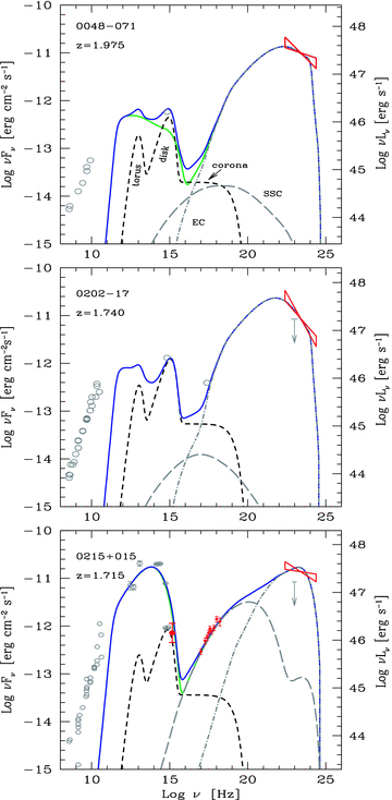
SED of PKS 0048−071, 0202−17 and PKS 0215+015, together with the fitting models, with parameters listed in Table 4. Fermi and Swift data are indicated by dark grey symbols (red in the electronic version), while archival data (from NED) are in light grey. The short-dashed line is the emission from the IR torus, the accretion disc and its X-ray corona; the long-dashed line is the SSC contribution and the dot–dashed line is the EC emission. The solid light grey line (green in the electronic version) is the non-thermal flux produced by the jet, the solid dark grey line (blue in the electronic version) is the sum of the non-thermal and thermal components.

Open in new tabDownload slide

Figure 2

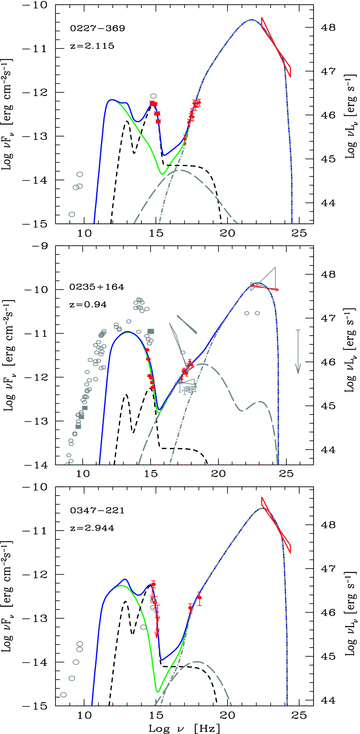
SED of PKS 0227−369, AO 0235+164 and PKS 0347−221. Symbols and lines as in Fig. 1.

Open in new tabDownload slide

Figure 3

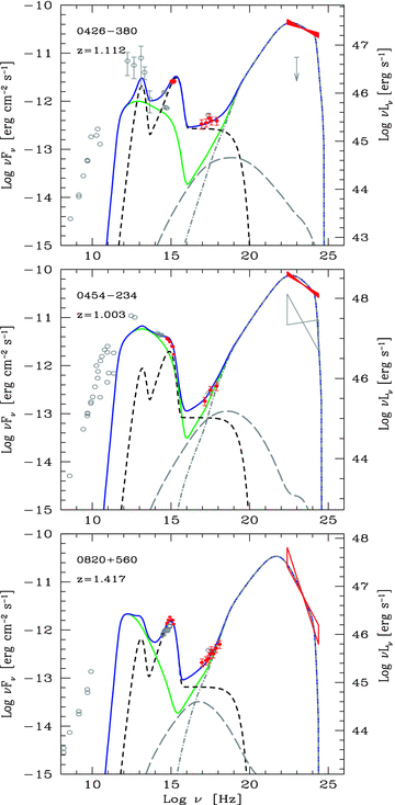
SED of PKS 0426−380, PKS 0445−234 and PKS 0820+560. Symbols and lines as in Fig. 1.

Open in new tabDownload slide

Figure 4

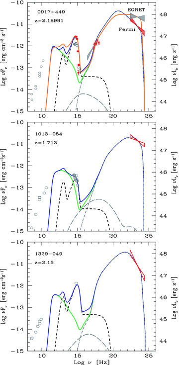
SED of 0917+449 = S4 0920+44, 1013−054 and 1329−049. Symbols and lines as in Fig. 1. For PKS 0917+449 we show two models, corresponding to the Fermi/Swift data and to the older EGRET data.

Open in new tabDownload slide

Figure 5

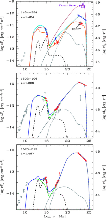
SED of 1424−354, PKS 1502+106, PKS 1520+319. Symbols and lines as in Fig. 1.

Open in new tabDownload slide

Figure 6

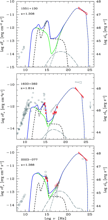
SED of PKS 1551+130, PKS 1633+382 and PKS 2023−077. Symbols and lines as in Fig. 1.

Open in new tabDownload slide

Figure 7

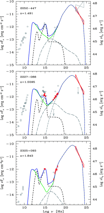
SED of PKS 2052−47, PKS 2227−088, PKS 2052−447 and PKS 2325+093. Symbols and lines as in Fig. 1.

Open in new tabDownload slide

Figure 8

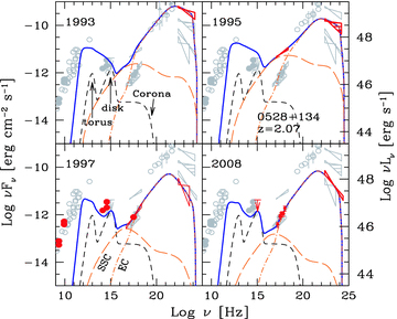
SED of PKS 0528+134 at four epochs. For the first three, the γ-ray data come from EGRET. For the 2008 SED, the γ-ray data are from Fermi. Symbols and lines as in Fig. 1.

Open in new tabDownload slide

Figure 9

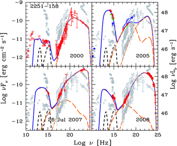
SED of PKS 2251−158 = 3C 454.3 at four epochs. For the 2007 July SED, γ-ray data come from AGILE (Vercellone et al. 2009). For the 2008 SED, the γ-ray data are from Fermi (Abdo et al. 2009b). Symbols and lines as in Fig. 1.

Open in new tabDownload slide

Table 4

Open in new tab

List of parameters used to construct the theoretical SED. Subscripts refer to the year of the corresponding SED or to an EGRET (E) state as opposed to a Fermi (F) state. Column [1]: name; column [2]: redshift; column [3]: dissipation radius in units of 10¹⁵ cm and (in parenthesis) in units of R_S; column [4]: black hole mass in solar masses; column [5]: size of the BLR in units of 10¹⁵ cm; column [6]: power injected in the blob calculated in the comoving frame, in units of 10⁴⁵ erg s⁻¹; column [7]: accretion disc luminosity in units of 10⁴⁵ erg s⁻¹ and (in parenthesis) in units of L_Edd; column [8]: magnetic field in Gauss; column [9]: bulk Lorentz factor at R_diss; column [10]: viewing angle in degrees; columns [11] and [12]: break and maximum random Lorentz factors of the injected electrons; columns [13] and [14]: slopes of the injected electron distribution [Q(γ)] below and above γ_b; for all cases the X-ray corona luminosity L_X= 0.3L_d. Its spectral shape is assumed to be ∝ν⁻¹ exp (−hν/150 keV).

Name [1]	z[2]	Rdiss[3]	M[4]	RBLR[5]	P′i[6]	Ld[7]	B[8]	Γ[9]	θv[10]	γb[11]	γmax[12]	s1[13]	s2[14]
0048−071	1.975	210 (700)	1e9	474	0.025	22.5 (0.15)	2.4	15.3	3	400	7e3	1	2.7
0202−17	1.74	300 (1000)	1e9	671	0.03	45 (0.3)	2.4	15	3	300	5e3	1	3.1
0215+015	1.715	900 (1500)	2e9	548	0.04	30 (0.1)	1.1	13	3	2.5e3	6e3	−1	3.5
0227−369	2.115	420 (700)	2e9	547	0.08	30 (0.1)	1.5	14	3	200	5e3	0	3.1
0235+164	0.94	132 (440)	1e9	212	0.042	4.5 (0.03)	2.9	12.1	3	400	2.7e3	−1	2.1
0347−211	2.944	750 (500)	5e9	866	0.12	75 (0.1)	1.5	12.9	3	500	3e3	−1	3.0
0426−380	1.112	156 (1300)	4e8	600	0.018	36 (0.6)	1.7	13	3	300	6e3	−1	2.4
0454−234	1.003	338 (450)	2.5e9	433	0.027	18.8 (0.05)	3	12.2	3	330	4e3	−1	2.4
0528+13493	2.04	540 (1800)	1e9	866	1.1	75 (0.5)	1.7	15	3	150	4e3	−1	2.3
0528+13495	2.04	315 (1050)	1e9	866	0.45	75 (0.5)	3.5	13	3	160	5e3	−1	2.3
0528+13497	2.04	300 (1000)	1e9	866	0.1	75 (0.5)	3.6	13	3	120	3e3	−1	3.0
0528+13408	2.04	420 (1400)	1e9	866	0.13	75 (0.5)	2.6	13	3	150	3e3	−1	2.8
0820+560	1.417	261 (580)	1.5e9	581	0.023	34 (0.15)	3.1	13.9	3	220	3e3	0	3.4
0917−449F	2.1899	900 (500)	6e9	1341	0.1	180 (0.2)	1.95	12.9	3	50	4e3	−1	2.6
0917−449E	2.1899	900 (500)	6e9	1341	0.1	180 (0.2)	1.95	12.9	3	30	4e3	−1	2
1013+054	1.713	252 (420)	2e9	300	0.036	9 (0.03)	1.7	11.8	3	500	3e3	1	2.4
1329−049	2.15	450 (1000)	1.5e9	822	0.07	67.5 (0.3)	1.4	15	3	300	5e3	1	3.3
1454−	1.424	150 (250)	2e9	671	0.05	45 (0.15)	4.9	15	3	450	3e3	−1	2.4
1454−	1.424	240 (400)	2e9	671	0.025	45 (0.15)	3.9	11.5	3	100	3e3	−1	2.0
1454−	1.424	150 (250)	2e9	671	0.25	45 (0.15)	2.0	20.	3	1e3	4e3	−1	2.0
1502+106	1.839	450 (500)	3e9	764	0.16	58.5 (0.13)	2.8	12.9	3	600	4e3	−1	2.1
1520+319	1.487	1500 (2000)	2.5e9	237	0.04	5.6 (0.015)	0.06	15	3	2e3	3e4	0.8	2.6
1551+130	1.308	330 (1100)	1e9	755	0.02	57 (0.38)	2.0	13	3	200	6e3	−1	2.4
1633+382	1.814	750 (500)	5e9	866	0.07	75 (0.1)	1.5	12.9	3	230	6e3	0	2.9
2023−077	1.388	378 (420)	3e9	474	0.07	22.5 (0.05)	1.8	11.8	3	350	4e3	0	2.6
2052−47	1.4910	210 (700)	1e9	612	0.045	37.5 (0.25)	2.6	13	3	100	7e3	−1	3.0
2227−088	1.5595	211 (470)	1.5e9	497	0.06	24.8 (0.11)	3.3	12	3	200	5e3	0.5	3.2
2251+15800	0.859	300 (1000)	1e9	548	0.05	30 (0.2)	3.3	13	3	40	7e3	0.5	2.4
2251+15805	0.859	120 (400)	1e9	548	0.15	30 (0.2)	15.5	11.5	3	600	1.5e3	0	3.5
2251+15807	0.859	270 (900)	1e9	548	0.22	30 (0.2)	3.6	13	3	20	3.5e3	1.6	1.6
2251+15808	0.859	240 (800)	1e9	548	0.14	30 (0.2)	4.1	13	3	250	4e3	1	2.7
2325+093	1.843	420 (1400)	1e9	671	0.08	45 (0.3)	1.6	16	3	190	5e3	0	3.5

Name [1]	z[2]	Rdiss[3]	M[4]	RBLR[5]	P′i[6]	Ld[7]	B[8]	Γ[9]	θv[10]	γb[11]	γmax[12]	s1[13]	s2[14]
0048−071	1.975	210 (700)	1e9	474	0.025	22.5 (0.15)	2.4	15.3	3	400	7e3	1	2.7
0202−17	1.74	300 (1000)	1e9	671	0.03	45 (0.3)	2.4	15	3	300	5e3	1	3.1
0215+015	1.715	900 (1500)	2e9	548	0.04	30 (0.1)	1.1	13	3	2.5e3	6e3	−1	3.5
0227−369	2.115	420 (700)	2e9	547	0.08	30 (0.1)	1.5	14	3	200	5e3	0	3.1
0235+164	0.94	132 (440)	1e9	212	0.042	4.5 (0.03)	2.9	12.1	3	400	2.7e3	−1	2.1
0347−211	2.944	750 (500)	5e9	866	0.12	75 (0.1)	1.5	12.9	3	500	3e3	−1	3.0
0426−380	1.112	156 (1300)	4e8	600	0.018	36 (0.6)	1.7	13	3	300	6e3	−1	2.4
0454−234	1.003	338 (450)	2.5e9	433	0.027	18.8 (0.05)	3	12.2	3	330	4e3	−1	2.4
0528+13493	2.04	540 (1800)	1e9	866	1.1	75 (0.5)	1.7	15	3	150	4e3	−1	2.3
0528+13495	2.04	315 (1050)	1e9	866	0.45	75 (0.5)	3.5	13	3	160	5e3	−1	2.3
0528+13497	2.04	300 (1000)	1e9	866	0.1	75 (0.5)	3.6	13	3	120	3e3	−1	3.0
0528+13408	2.04	420 (1400)	1e9	866	0.13	75 (0.5)	2.6	13	3	150	3e3	−1	2.8
0820+560	1.417	261 (580)	1.5e9	581	0.023	34 (0.15)	3.1	13.9	3	220	3e3	0	3.4
0917−449F	2.1899	900 (500)	6e9	1341	0.1	180 (0.2)	1.95	12.9	3	50	4e3	−1	2.6
0917−449E	2.1899	900 (500)	6e9	1341	0.1	180 (0.2)	1.95	12.9	3	30	4e3	−1	2
1013+054	1.713	252 (420)	2e9	300	0.036	9 (0.03)	1.7	11.8	3	500	3e3	1	2.4
1329−049	2.15	450 (1000)	1.5e9	822	0.07	67.5 (0.3)	1.4	15	3	300	5e3	1	3.3
1454−	1.424	150 (250)	2e9	671	0.05	45 (0.15)	4.9	15	3	450	3e3	−1	2.4
1454−	1.424	240 (400)	2e9	671	0.025	45 (0.15)	3.9	11.5	3	100	3e3	−1	2.0
1454−	1.424	150 (250)	2e9	671	0.25	45 (0.15)	2.0	20.	3	1e3	4e3	−1	2.0
1502+106	1.839	450 (500)	3e9	764	0.16	58.5 (0.13)	2.8	12.9	3	600	4e3	−1	2.1
1520+319	1.487	1500 (2000)	2.5e9	237	0.04	5.6 (0.015)	0.06	15	3	2e3	3e4	0.8	2.6
1551+130	1.308	330 (1100)	1e9	755	0.02	57 (0.38)	2.0	13	3	200	6e3	−1	2.4
1633+382	1.814	750 (500)	5e9	866	0.07	75 (0.1)	1.5	12.9	3	230	6e3	0	2.9
2023−077	1.388	378 (420)	3e9	474	0.07	22.5 (0.05)	1.8	11.8	3	350	4e3	0	2.6
2052−47	1.4910	210 (700)	1e9	612	0.045	37.5 (0.25)	2.6	13	3	100	7e3	−1	3.0
2227−088	1.5595	211 (470)	1.5e9	497	0.06	24.8 (0.11)	3.3	12	3	200	5e3	0.5	3.2
2251+15800	0.859	300 (1000)	1e9	548	0.05	30 (0.2)	3.3	13	3	40	7e3	0.5	2.4
2251+15805	0.859	120 (400)	1e9	548	0.15	30 (0.2)	15.5	11.5	3	600	1.5e3	0	3.5
2251+15807	0.859	270 (900)	1e9	548	0.22	30 (0.2)	3.6	13	3	20	3.5e3	1.6	1.6
2251+15808	0.859	240 (800)	1e9	548	0.14	30 (0.2)	4.1	13	3	250	4e3	1	2.7
2325+093	1.843	420 (1400)	1e9	671	0.08	45 (0.3)	1.6	16	3	190	5e3	0	3.5

Table 4

Open in new tab

List of parameters used to construct the theoretical SED. Subscripts refer to the year of the corresponding SED or to an EGRET (E) state as opposed to a Fermi (F) state. Column [1]: name; column [2]: redshift; column [3]: dissipation radius in units of 10¹⁵ cm and (in parenthesis) in units of R_S; column [4]: black hole mass in solar masses; column [5]: size of the BLR in units of 10¹⁵ cm; column [6]: power injected in the blob calculated in the comoving frame, in units of 10⁴⁵ erg s⁻¹; column [7]: accretion disc luminosity in units of 10⁴⁵ erg s⁻¹ and (in parenthesis) in units of L_Edd; column [8]: magnetic field in Gauss; column [9]: bulk Lorentz factor at R_diss; column [10]: viewing angle in degrees; columns [11] and [12]: break and maximum random Lorentz factors of the injected electrons; columns [13] and [14]: slopes of the injected electron distribution [Q(γ)] below and above γ_b; for all cases the X-ray corona luminosity L_X= 0.3L_d. Its spectral shape is assumed to be ∝ν⁻¹ exp (−hν/150 keV).

Name [1]	z[2]	Rdiss[3]	M[4]	RBLR[5]	P′i[6]	Ld[7]	B[8]	Γ[9]	θv[10]	γb[11]	γmax[12]	s1[13]	s2[14]
0048−071	1.975	210 (700)	1e9	474	0.025	22.5 (0.15)	2.4	15.3	3	400	7e3	1	2.7
0202−17	1.74	300 (1000)	1e9	671	0.03	45 (0.3)	2.4	15	3	300	5e3	1	3.1
0215+015	1.715	900 (1500)	2e9	548	0.04	30 (0.1)	1.1	13	3	2.5e3	6e3	−1	3.5
0227−369	2.115	420 (700)	2e9	547	0.08	30 (0.1)	1.5	14	3	200	5e3	0	3.1
0235+164	0.94	132 (440)	1e9	212	0.042	4.5 (0.03)	2.9	12.1	3	400	2.7e3	−1	2.1
0347−211	2.944	750 (500)	5e9	866	0.12	75 (0.1)	1.5	12.9	3	500	3e3	−1	3.0
0426−380	1.112	156 (1300)	4e8	600	0.018	36 (0.6)	1.7	13	3	300	6e3	−1	2.4
0454−234	1.003	338 (450)	2.5e9	433	0.027	18.8 (0.05)	3	12.2	3	330	4e3	−1	2.4
0528+13493	2.04	540 (1800)	1e9	866	1.1	75 (0.5)	1.7	15	3	150	4e3	−1	2.3
0528+13495	2.04	315 (1050)	1e9	866	0.45	75 (0.5)	3.5	13	3	160	5e3	−1	2.3
0528+13497	2.04	300 (1000)	1e9	866	0.1	75 (0.5)	3.6	13	3	120	3e3	−1	3.0
0528+13408	2.04	420 (1400)	1e9	866	0.13	75 (0.5)	2.6	13	3	150	3e3	−1	2.8
0820+560	1.417	261 (580)	1.5e9	581	0.023	34 (0.15)	3.1	13.9	3	220	3e3	0	3.4
0917−449F	2.1899	900 (500)	6e9	1341	0.1	180 (0.2)	1.95	12.9	3	50	4e3	−1	2.6
0917−449E	2.1899	900 (500)	6e9	1341	0.1	180 (0.2)	1.95	12.9	3	30	4e3	−1	2
1013+054	1.713	252 (420)	2e9	300	0.036	9 (0.03)	1.7	11.8	3	500	3e3	1	2.4
1329−049	2.15	450 (1000)	1.5e9	822	0.07	67.5 (0.3)	1.4	15	3	300	5e3	1	3.3
1454−	1.424	150 (250)	2e9	671	0.05	45 (0.15)	4.9	15	3	450	3e3	−1	2.4
1454−	1.424	240 (400)	2e9	671	0.025	45 (0.15)	3.9	11.5	3	100	3e3	−1	2.0
1454−	1.424	150 (250)	2e9	671	0.25	45 (0.15)	2.0	20.	3	1e3	4e3	−1	2.0
1502+106	1.839	450 (500)	3e9	764	0.16	58.5 (0.13)	2.8	12.9	3	600	4e3	−1	2.1
1520+319	1.487	1500 (2000)	2.5e9	237	0.04	5.6 (0.015)	0.06	15	3	2e3	3e4	0.8	2.6
1551+130	1.308	330 (1100)	1e9	755	0.02	57 (0.38)	2.0	13	3	200	6e3	−1	2.4
1633+382	1.814	750 (500)	5e9	866	0.07	75 (0.1)	1.5	12.9	3	230	6e3	0	2.9
2023−077	1.388	378 (420)	3e9	474	0.07	22.5 (0.05)	1.8	11.8	3	350	4e3	0	2.6
2052−47	1.4910	210 (700)	1e9	612	0.045	37.5 (0.25)	2.6	13	3	100	7e3	−1	3.0
2227−088	1.5595	211 (470)	1.5e9	497	0.06	24.8 (0.11)	3.3	12	3	200	5e3	0.5	3.2
2251+15800	0.859	300 (1000)	1e9	548	0.05	30 (0.2)	3.3	13	3	40	7e3	0.5	2.4
2251+15805	0.859	120 (400)	1e9	548	0.15	30 (0.2)	15.5	11.5	3	600	1.5e3	0	3.5
2251+15807	0.859	270 (900)	1e9	548	0.22	30 (0.2)	3.6	13	3	20	3.5e3	1.6	1.6
2251+15808	0.859	240 (800)	1e9	548	0.14	30 (0.2)	4.1	13	3	250	4e3	1	2.7
2325+093	1.843	420 (1400)	1e9	671	0.08	45 (0.3)	1.6	16	3	190	5e3	0	3.5

Name [1]	z[2]	Rdiss[3]	M[4]	RBLR[5]	P′i[6]	Ld[7]	B[8]	Γ[9]	θv[10]	γb[11]	γmax[12]	s1[13]	s2[14]
0048−071	1.975	210 (700)	1e9	474	0.025	22.5 (0.15)	2.4	15.3	3	400	7e3	1	2.7
0202−17	1.74	300 (1000)	1e9	671	0.03	45 (0.3)	2.4	15	3	300	5e3	1	3.1
0215+015	1.715	900 (1500)	2e9	548	0.04	30 (0.1)	1.1	13	3	2.5e3	6e3	−1	3.5
0227−369	2.115	420 (700)	2e9	547	0.08	30 (0.1)	1.5	14	3	200	5e3	0	3.1
0235+164	0.94	132 (440)	1e9	212	0.042	4.5 (0.03)	2.9	12.1	3	400	2.7e3	−1	2.1
0347−211	2.944	750 (500)	5e9	866	0.12	75 (0.1)	1.5	12.9	3	500	3e3	−1	3.0
0426−380	1.112	156 (1300)	4e8	600	0.018	36 (0.6)	1.7	13	3	300	6e3	−1	2.4
0454−234	1.003	338 (450)	2.5e9	433	0.027	18.8 (0.05)	3	12.2	3	330	4e3	−1	2.4
0528+13493	2.04	540 (1800)	1e9	866	1.1	75 (0.5)	1.7	15	3	150	4e3	−1	2.3
0528+13495	2.04	315 (1050)	1e9	866	0.45	75 (0.5)	3.5	13	3	160	5e3	−1	2.3
0528+13497	2.04	300 (1000)	1e9	866	0.1	75 (0.5)	3.6	13	3	120	3e3	−1	3.0
0528+13408	2.04	420 (1400)	1e9	866	0.13	75 (0.5)	2.6	13	3	150	3e3	−1	2.8
0820+560	1.417	261 (580)	1.5e9	581	0.023	34 (0.15)	3.1	13.9	3	220	3e3	0	3.4
0917−449F	2.1899	900 (500)	6e9	1341	0.1	180 (0.2)	1.95	12.9	3	50	4e3	−1	2.6
0917−449E	2.1899	900 (500)	6e9	1341	0.1	180 (0.2)	1.95	12.9	3	30	4e3	−1	2
1013+054	1.713	252 (420)	2e9	300	0.036	9 (0.03)	1.7	11.8	3	500	3e3	1	2.4
1329−049	2.15	450 (1000)	1.5e9	822	0.07	67.5 (0.3)	1.4	15	3	300	5e3	1	3.3
1454−	1.424	150 (250)	2e9	671	0.05	45 (0.15)	4.9	15	3	450	3e3	−1	2.4
1454−	1.424	240 (400)	2e9	671	0.025	45 (0.15)	3.9	11.5	3	100	3e3	−1	2.0
1454−	1.424	150 (250)	2e9	671	0.25	45 (0.15)	2.0	20.	3	1e3	4e3	−1	2.0
1502+106	1.839	450 (500)	3e9	764	0.16	58.5 (0.13)	2.8	12.9	3	600	4e3	−1	2.1
1520+319	1.487	1500 (2000)	2.5e9	237	0.04	5.6 (0.015)	0.06	15	3	2e3	3e4	0.8	2.6
1551+130	1.308	330 (1100)	1e9	755	0.02	57 (0.38)	2.0	13	3	200	6e3	−1	2.4
1633+382	1.814	750 (500)	5e9	866	0.07	75 (0.1)	1.5	12.9	3	230	6e3	0	2.9
2023−077	1.388	378 (420)	3e9	474	0.07	22.5 (0.05)	1.8	11.8	3	350	4e3	0	2.6
2052−47	1.4910	210 (700)	1e9	612	0.045	37.5 (0.25)	2.6	13	3	100	7e3	−1	3.0
2227−088	1.5595	211 (470)	1.5e9	497	0.06	24.8 (0.11)	3.3	12	3	200	5e3	0.5	3.2
2251+15800	0.859	300 (1000)	1e9	548	0.05	30 (0.2)	3.3	13	3	40	7e3	0.5	2.4
2251+15805	0.859	120 (400)	1e9	548	0.15	30 (0.2)	15.5	11.5	3	600	1.5e3	0	3.5
2251+15807	0.859	270 (900)	1e9	548	0.22	30 (0.2)	3.6	13	3	20	3.5e3	1.6	1.6
2251+15808	0.859	240 (800)	1e9	548	0.14	30 (0.2)	4.1	13	3	250	4e3	1	2.7
2325+093	1.843	420 (1400)	1e9	671	0.08	45 (0.3)	1.6	16	3	190	5e3	0	3.5

Table 5

Open in new tab

Jet power in the form of radiation, Poynting flux, bulk motion of electrons and protons (assuming one proton per emitting electron). Subscripts refer to the year of the corresponding SED or to an EGRET (E) state as opposed to a Fermi (F) state.

Name	logPr	logPB	logPe	logPp
PKS 0048−071	45.75	45.35	44.69	47.10
PKS 0202−17	45.80	45.65	44.80	47.31
PKS 0215+015	45.81	45.78	44.86	46.09
PKS 0227−369	46.18	45.49	44.97	47.34
AO 0235+164	45.78	44.97	44.61	46.60
PKS 0347−211	46.30	45.91	44.55	46.92
PKS 0426−380	45.48	44.67	44.30	46.36
PKS 0454−234	45.60	45.80	44.16	46.40
PKS 0528+13493	46.32	45.88	45.12	47.52
PKS 0528+13495	46.19	45.88	45.22	47.61
PKS 0528+13497	46.87	45.88	45.59	47.94
PKS 0528+13408	47.39	45.86	45.87	48.31
TXS 0820+560	45.60	45.75	44.57	46.85
TXS 0917+449F	46.20	46.29	45.00	47.57
TXS 0917+449E	46.20	46.29	44.87	47.43
TXS 1013+054	45.68	45.02	44.66	46.99
PKS 1329−049	46.18	45.53	45.07	47.65
PKS 1454−	46.04	45.65	44.59	46.80
PKS 1454−	45.50	45.65	44.38	46.53
PKS 1454−	47.01	45.13	45.20	47.47
PKS 1502+106	46.43	46.12	44.63	46.91
TXS 1520+319	45.91	43.84	45.22	46.50
PKS 1551+130	45.53	45.45	44.21	46.48
TXS 1633+382	46.06	45.91	44.60	47.05
PKS 2023−077	45.98	45.41	44.65	46.87
PKS 2052−47	45.84	45.27	45.01	47.24
PKS 2227−088	45.89	45.40	45.07	47.29
PKS 2251+15800	45.87	45.78	45.11	47.56
PKS 2251+15805	46.24	46.34	44.84	47.12
PKS 2251+15807	46.53	45.78	45.61	48.24
PKS 2251+15808	46.33	45.78	45.43	47.87
PKS 2325+093	46.30	45.65	45.06	47.51

Name	logPr	logPB	logPe	logPp
PKS 0048−071	45.75	45.35	44.69	47.10
PKS 0202−17	45.80	45.65	44.80	47.31
PKS 0215+015	45.81	45.78	44.86	46.09
PKS 0227−369	46.18	45.49	44.97	47.34
AO 0235+164	45.78	44.97	44.61	46.60
PKS 0347−211	46.30	45.91	44.55	46.92
PKS 0426−380	45.48	44.67	44.30	46.36
PKS 0454−234	45.60	45.80	44.16	46.40
PKS 0528+13493	46.32	45.88	45.12	47.52
PKS 0528+13495	46.19	45.88	45.22	47.61
PKS 0528+13497	46.87	45.88	45.59	47.94
PKS 0528+13408	47.39	45.86	45.87	48.31
TXS 0820+560	45.60	45.75	44.57	46.85
TXS 0917+449F	46.20	46.29	45.00	47.57
TXS 0917+449E	46.20	46.29	44.87	47.43
TXS 1013+054	45.68	45.02	44.66	46.99
PKS 1329−049	46.18	45.53	45.07	47.65
PKS 1454−	46.04	45.65	44.59	46.80
PKS 1454−	45.50	45.65	44.38	46.53
PKS 1454−	47.01	45.13	45.20	47.47
PKS 1502+106	46.43	46.12	44.63	46.91
TXS 1520+319	45.91	43.84	45.22	46.50
PKS 1551+130	45.53	45.45	44.21	46.48
TXS 1633+382	46.06	45.91	44.60	47.05
PKS 2023−077	45.98	45.41	44.65	46.87
PKS 2052−47	45.84	45.27	45.01	47.24
PKS 2227−088	45.89	45.40	45.07	47.29
PKS 2251+15800	45.87	45.78	45.11	47.56
PKS 2251+15805	46.24	46.34	44.84	47.12
PKS 2251+15807	46.53	45.78	45.61	48.24
PKS 2251+15808	46.33	45.78	45.43	47.87
PKS 2325+093	46.30	45.65	45.06	47.51

Table 5

Open in new tab

Jet power in the form of radiation, Poynting flux, bulk motion of electrons and protons (assuming one proton per emitting electron). Subscripts refer to the year of the corresponding SED or to an EGRET (E) state as opposed to a Fermi (F) state.

Name	logPr	logPB	logPe	logPp
PKS 0048−071	45.75	45.35	44.69	47.10
PKS 0202−17	45.80	45.65	44.80	47.31
PKS 0215+015	45.81	45.78	44.86	46.09
PKS 0227−369	46.18	45.49	44.97	47.34
AO 0235+164	45.78	44.97	44.61	46.60
PKS 0347−211	46.30	45.91	44.55	46.92
PKS 0426−380	45.48	44.67	44.30	46.36
PKS 0454−234	45.60	45.80	44.16	46.40
PKS 0528+13493	46.32	45.88	45.12	47.52
PKS 0528+13495	46.19	45.88	45.22	47.61
PKS 0528+13497	46.87	45.88	45.59	47.94
PKS 0528+13408	47.39	45.86	45.87	48.31
TXS 0820+560	45.60	45.75	44.57	46.85
TXS 0917+449F	46.20	46.29	45.00	47.57
TXS 0917+449E	46.20	46.29	44.87	47.43
TXS 1013+054	45.68	45.02	44.66	46.99
PKS 1329−049	46.18	45.53	45.07	47.65
PKS 1454−	46.04	45.65	44.59	46.80
PKS 1454−	45.50	45.65	44.38	46.53
PKS 1454−	47.01	45.13	45.20	47.47
PKS 1502+106	46.43	46.12	44.63	46.91
TXS 1520+319	45.91	43.84	45.22	46.50
PKS 1551+130	45.53	45.45	44.21	46.48
TXS 1633+382	46.06	45.91	44.60	47.05
PKS 2023−077	45.98	45.41	44.65	46.87
PKS 2052−47	45.84	45.27	45.01	47.24
PKS 2227−088	45.89	45.40	45.07	47.29
PKS 2251+15800	45.87	45.78	45.11	47.56
PKS 2251+15805	46.24	46.34	44.84	47.12
PKS 2251+15807	46.53	45.78	45.61	48.24
PKS 2251+15808	46.33	45.78	45.43	47.87
PKS 2325+093	46.30	45.65	45.06	47.51

Name	logPr	logPB	logPe	logPp
PKS 0048−071	45.75	45.35	44.69	47.10
PKS 0202−17	45.80	45.65	44.80	47.31
PKS 0215+015	45.81	45.78	44.86	46.09
PKS 0227−369	46.18	45.49	44.97	47.34
AO 0235+164	45.78	44.97	44.61	46.60
PKS 0347−211	46.30	45.91	44.55	46.92
PKS 0426−380	45.48	44.67	44.30	46.36
PKS 0454−234	45.60	45.80	44.16	46.40
PKS 0528+13493	46.32	45.88	45.12	47.52
PKS 0528+13495	46.19	45.88	45.22	47.61
PKS 0528+13497	46.87	45.88	45.59	47.94
PKS 0528+13408	47.39	45.86	45.87	48.31
TXS 0820+560	45.60	45.75	44.57	46.85
TXS 0917+449F	46.20	46.29	45.00	47.57
TXS 0917+449E	46.20	46.29	44.87	47.43
TXS 1013+054	45.68	45.02	44.66	46.99
PKS 1329−049	46.18	45.53	45.07	47.65
PKS 1454−	46.04	45.65	44.59	46.80
PKS 1454−	45.50	45.65	44.38	46.53
PKS 1454−	47.01	45.13	45.20	47.47
PKS 1502+106	46.43	46.12	44.63	46.91
TXS 1520+319	45.91	43.84	45.22	46.50
PKS 1551+130	45.53	45.45	44.21	46.48
TXS 1633+382	46.06	45.91	44.60	47.05
PKS 2023−077	45.98	45.41	44.65	46.87
PKS 2052−47	45.84	45.27	45.01	47.24
PKS 2227−088	45.89	45.40	45.07	47.29
PKS 2251+15800	45.87	45.78	45.11	47.56
PKS 2251+15805	46.24	46.34	44.84	47.12
PKS 2251+15807	46.53	45.78	45.61	48.24
PKS 2251+15808	46.33	45.78	45.43	47.87
PKS 2325+093	46.30	45.65	45.06	47.51

This fact, together with the theoretical considerations mentioned in the previous section, allow us to consider the optical–UV emission of nearly half of our blazars as due to the accretion disc emission. Among the sources with UVOT data exceptions are 0215+015, 0235+164, 0454−234, 0528+134, 1454−354, 2251−158 and 2325+093. For these sources either the non-thermal continuum dominates the flux, or the quality of the data is not sufficient to discriminate between the thermal and the non-thermal processes. For them, the black hole mass and disc luminosity has been chosen (when summed to the non-thermal emission) not to overproduce the observed flux.

6.1 Black hole masses, accretion and outflow rates

The derived black hole masses are in the range (1–6) × 10⁹ M_⊙ (Fig. 11), and the disc luminosities, in Eddington units, cluster around L_d/L_Edd∼ 0.1–0.3 (see Fig. 10). Fig. 11 shows the accretion and outflow mass rates (in units of M_⊙ yr⁻¹) and their ratio. All our sources requires more than 1 M_⊙ yr⁻¹ of accreting mass, while the outflow rate is a factor of 0.01–0.1 smaller. This can be understood in simple terms, considering that in matter dominated jets and then

5

Figure 11

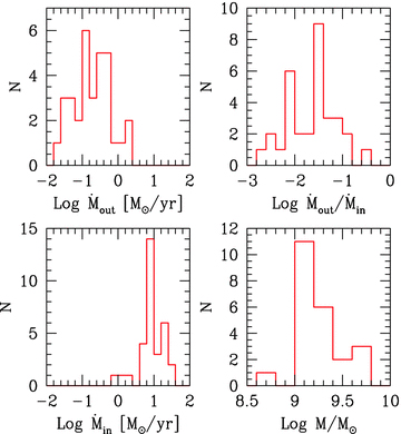
Histograms of the outflowing (top left) mass rate; the accretion mass rate (bottom left) and their ratio (top right). On the bottom right we show the distribution of black hole masses found in this paper.

Open in new tabDownload slide

Figure 10

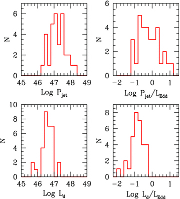
Histograms of the total jet power and the accretion disc luminosity, both in cgs units (left) and in Eddington units (right).

Open in new tabDownload slide

6.2 Jet power

Table 5 lists the power carried by the jet in the form of radiation (P_r), magnetic field (P_B), electrons (P_e) and protons (P_p, assuming one proton per emitting electron). All the powers are calculated as

6

where U_i is the energy density of the i component.

The total power carried by the jet is often larger than the disc luminosity, and sometimes exceeds the Eddington luminosity (see Figs 10 and 12). In Fig. 12 we compare P_j as a function of L_d for our sources with the FSRQs and BL Lacs analysed in CG08 and with the FSRQs analysed in M08. As can be seen, the blazars analysed in CG08 and M08 tend to have larger jet powers with respect to disc luminosities than the blazars presented here. This can be partly understood considering that a large fraction of the blazars in CG08 were EGRET sources, and the γ-ray data correspond to high state of the sources. In our sample, instead, the γ-ray luminosity, derived by the averageγ-ray flux seen by Fermi, is considerably smaller than the maximum values seen by EGRET (see Fig. 8 as illustrative example). The smaller electromagnetic power output implies that also the kinetic power carried by the jet is smaller. The blazars considered in M08 (see also Sambruna et al. 2007; Ghisellini 2009), instead, lack γ-ray data, and the estimates were based on fitting the SED up to the Swift-XRT energy range. Several of them showed a very hard X-ray spectrum, suggesting a peak in the 1–10 MeV region of the spectrum. MeV blazars of this kind, peaking at energies significantly smaller than 100 MeV, may not be easily observable by Fermi, and could be among the most luminous blazars1 (according to the blazar sequence; Fossati et al. 1998). The jet powers calculated here may not correspond to the ‘very high states’ of blazars as seen by EGRET. They are therefore more representative of a typical blazar state, but we have to remember that when constructing a list of variable sources (even with a more sensitive instrument) high states are always overrepresented. What is confirmed with these new data is that, at least occasionally, the jet is more powerful than L_d.

Figure 12

The jet power as a function of the accretion disc luminosity of different blazar samples. Black filled circles: our sources; empty squares: FSRQs analysed in CG08; stars: BL Lac objects analysed in CG08; empty circles: FSRQs analysed in M08. 3C 273 and PKS 1510−089 are labelled, to show their position in this plane (see text).

Open in new tabDownload slide

We can also compare the fraction of the total jet power carried in radiation (ε_r), magnetic field (ε_B), and electrons (ε_e) with the sample of blazars studied in CG08. This is done in Fig. 13, showing a rough consistency with the blazars in CG08.

Figure 13

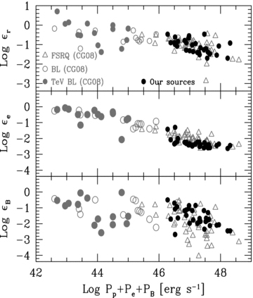
The fraction of L_jet radiated (ε_r, top panel), in relativistic leptons (ε_e, mid panel) and in magnetic fields (ε_B, bottom panel) as functions of P_j=Pp +P_e+P_B. Our sources (black circles) are compared to the FSRQs (grey triangles), BL Lacs (grey empty circles) and TeV BL Lacs (grey filled circles) of the blazar sample studied in CG8.

Open in new tabDownload slide

6.3 Emission mechanisms

The location of the dissipation region is almost always within the BLR (exceptions are 0215+015 and 1520+319), that provides most of the seed photons scattered at high frequencies. The main emission process are then synchrotron and thermal emission from the accretion disc for the low-frequency parts, and EC for the hard X-rays and the γ-ray part of the spectrum. The X-ray corona and the SSC flux marginally contribute to the soft X-ray part of the SED. The IR radiation reprocessed by the torus can in some case dominate the far-IR flux, but the scarcity of data in this frequency window does not allow to fully assess its importance. Note that when R_diss < R_BLR, the overall non-thermal emission is rather insensitive to the presence/absence of the IR torus, since the bulk of the seed photons is provided by the broad lines. However, for 0215+015 and 1520+319, the location of the dissipation region is beyond the BLR, and for these two sources the EC process with the IR radiation of the torus is crucial to explain their SED. Since their dissipation region is beyond the BLR, the corresponding energy densities in radiation and fields are smaller than in the other sources, as can be seen in the top panel of Fig. 14. Furthermore, the smaller U_r+U_B implies a slower cooling, and thus a larger γ_cool (bottom panel of Fig. 14).

Figure 14

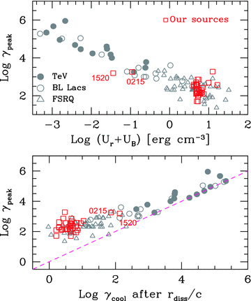
Top: γ_peak versus U_B+U′_r. Bottom: γ_peak versus γ_cool calculated after one light crossing time. The dashed line indicates equality. See text for details. In both panels the grey symbols are the blazars studied in CG08. The two sources outside the cluster of the other ones are PKS 0215+015 and TXS 1520+319, as labelled. These are the only two sources with R_diss > R_BLR and this implies a reduced energy density (in radiation and magnetic field) and therefore a larger γ_cool.

Open in new tabDownload slide

6.4 Particle distribution

The lower end of the emitting particle distribution is usually the bottleneck to reliably calculate how many particle the jet carries, and hence its power. This is because low-energy electrons emit, by synchrotron, in the self-absorbed, not visible, regime, and, by SSC, they contribute in a region of the SED usually dominated by synchrotron or by the accretion disc. There are however several cases where the X-ray data can be convincingly fitted by the EC mechanism, and in these cases the IC radiation produced by these low-energy electrons is dominating the observed flux. These are the cases where the X-ray spectral shape is very hard, especially at lower frequencies, excluding SSC as the main contributor to the observed flux. As examples, see the BeppoSAX spectrum of 2251−158 in the year 2000, or the XRT spectrum of 2325+093. These are the cases where the N(γ) distribution can be reliably determined even in its low-energy part. Theoretically, as an outcome of the model assumption, we can also calculate the random Lorentz factor of the electrons cooling in one light crossing time. This depends on the amount of radiative cooling, in turn depending on the bulk Lorentz factor, the magnetic field and the amount of external radiation. Fig. 14 shows the values of γ_cool (as a function of the peak energy γ_peak) for our sources. Since we are dealing with very powerful blazars, where the cooling is strong, the derived values are particularly small, of the order of 1–10. This ensure that N(γ) ∝γ⁻² between γ_cool and γ_b.

For all our sources the importance of the γ–γ→e^± process (which is included in our model) is very modest, and does not influence the observed spectrum.

6.5 Comparison with low power jets

Fig. 14 shows the value of the peak energy γ_peak (namely the random Lorentz factor of the electrons producing most of the emission at the two peaks of the SED) as a function of the total energy density (as seen in the comoving frame; upper panel) and as a function of γ_cool (calculated after one light crossing time r_diss/c; bottom panel). We have reported, for comparisons, the values obtained by CG08 for a sample of blazars including both powerful FSRQs and low power BL Lacs. As expected, the values for our blazar are consistent with those previously found by CG08 for powerful FSRQs. The bottom panel of Fig. 14 is a different version of the blazar sequence as originally proposed in Ghisellini et al. (1998) and shown in the upper panel. It suggests that γ_peak becomes equal to γ_cool when the cooling is weak, but it must be larger than γ_cool when the cooling is fast. Therefore, the position of the peaks of the SED of strong FSRQs is controlled by the injection function Q(γ) and its break at γ_b, that is proportional to γ_peak (the two energies are not exactly equal because of the assumed smoothly curved injection function, see GT09). In the slow cooling regime, instead (low power BL Lacs), γ_b becomes unimportant, and the particle distribution self-adjust itself. The new feature added here is the fact that in this case (i.e. slow cooling) the value of γ_peak=γ_cool depends also on the size of the source, and not only on the total energy density.

6.6 Multistates of specific sources

PKS 0528+134–Fig. 3 shows four states of this source, one of the best studied by EGRET, that was able to detect it at very different levels of γ-ray activity (see also Mukherjee et al. 1999 for a detailed analysis of the different states during the EGRET era). Keeping the black hole mass and the accretion rate fixed (so that also L_d and R_BLR are fixed), we tried to interpret the four different states changing a minimum number of parameters. Furthermore, the bulk Lorentz factor needs not to change. Indeed, the main changing parameters are (i) R_diss, implying a change of the magnetic field in the dissipation region (larger field at closer distances, according to a constant P_B, as listed in Table 5) and (ii) the power P′_i injected into the source in the form of relativistic electrons. The change in P′_i is the main responsible for the changes in the jet bulk kinetic power (factor of ∼5), that are sufficient to explain the rather dramatic changes in the observed SED. We had to change also the high-energy slope (s₂) of the injected electron distribution, and (but by a modest factor) γ₁ and γ_max. The changes of the magnetic field (factor of ∼2) are responsible for a very different contribution of the SSC flux in the X-ray band, dominated by this component in the SEDs of 1993 and 1995.

TXS 0917+449 = RGB 0920+446– In Fig. 4 we show two models for the SED of this source, corresponding to the combined Swift and Fermi data, and also to the old EGRET ones (for which there is a paucity of data). Therefore, the two models do not describe two different observed SEDs, but can illustrate how the model parameters have to change if only the γ-ray emission changes. In this case we have fixed, besides the black hole mass and accretion rate, also the location of the dissipation region, the magnetic field and the injected power. We only changed the high-energy slope of the injected electron distribution (s₂, from 2.6 to 2), and γ₁ (from 50 to 30). These changes are responsible for the (small) changes of the total bulk kinetic power of the jet.

PKS 1454−354–Fig. 5 shows three SEDs for this source, corresponding to three states already observed by Fermi and discussed in Abdo et al. (2009c). Fig. 5 reports the γ-ray data of the flare, of the ‘low’ state and of the intermediate γ-ray state that corresponds to the average flux reported in A09. Swift data corresponds to 2008 January and September. As for the other sources, we have tried to model the three states of the source assuming the same black hole mass and disc luminosity (hence the same R_BLR). Values of R_diss are constrained by the observed short variability time-scale of the γ-ray flux (Abdo et al. 2009c). We can reproduce the different source states by changing R_diss (factor of 2), P′_i (factor of 5), Γ (almost a factor of 2) and B (factor of ∼2.5). In addition, we had to adjust γ₁ and s₂. These changes of the physical parameters of the jet imply different jet powers (factor of ∼2 for P_B and ∼10 for the bulk kinetic jet power).

2251−158 = 3C 454.3–Fig. 9 shows four states of this source, one of the brightest AGILE blazars, and also detected, besides by Fermi, by EGRET. The first three SEDs have been discussed by Ghisellini et al. (2007), with the difference that at that time only an integrated AGILE flux was known, while now (Vercellone et al. 2009) the spectral analysis of the AGILE data yielded a spectrum rising in νF_ν. The fourth corresponds to the Fermi observation (with a flux slightly smaller than AGILE but with a steep slope). This blazars shows a rather dramatic variability at all frequencies, most notably in the optical band in 1995 (Fuhrmann et al. 2006; Giommi et al. 2006; Pian et al. 2006; Villata et al. 2006). Comparing the SED of the 2005 flare with the SED of 2000, the IR–optical flux increased by two orders of magnitude, while the hard X-rays flux increased by a factor of ∼10. Unfortunately, for the SED in 2005 there are no information about the γ-ray flux. Katarzynski & Ghisellini (2007) interpreted this behaviour (namely, more variability amplitude in the optical than at X-rays) suggesting that the main change was due to the location of the dissipation region in the jet, more internal in 2005. They showed that even with a constant jet power, and a constant bolometric luminosity, dramatic variations in specific bands were possible. The reason is that a more internal dissipation region may correspond to a larger magnetic field and a smaller bulk Lorentz factor (i.e. the jet may still be accelerating): the combination of these two key factors yields a larger magnetic energy density and a smaller external radiation field (since in the comoving frame it is less amplified by the smaller Γ). This in turn implies more synchrotron and less EC radiation. These ideas were later confirmed (Ghisellini et al. 2007) by the first AGILE observations, that caught the source in a bright γ-ray state and in a relatively faint optical state (compared to 1995). We here follow the same ideas, adopting a smaller R_diss and Γ for the 2005 state (see Table 4). The SED corresponding to the Fermi/Swift observations in 2008 confirms this scenario: the source is still much brighter in γ-rays than revealed by EGRET, but it is not exceptionally strong in optical. What is notably different, for the 2007 and 2008 states, is the slope of the γ-ray spectrum, which is flat (in νF_ν) for AGILE and steep for Fermi. We modelled the different 2007 and 2008 states with a different injected electron distribution, much flatter in 2007, leaving all other parameters unchanged. This implied a different number of emitting electrons, and a somewhat different jet power (see Table 5).

7 DISCUSSION

Several of our blazars have good Swift data that allowed to estimate the black hole mass and the disc luminosity. There are two reasons for the disc luminosity to emerge in the optical–UV range of the spectrum in these luminous sources: (i) according to the blazar sequence, and directly seen in the Fermi data, the high-energy spectrum is steep, implying a high-energy peak below the Fermi energy range. This implies that the corresponding synchrotron spectrum peaks in the IR band, with a relatively smaller contribution in the optical–UV. (ii) If highly luminous blazars have large black hole masses, then we expect relatively smaller magnetic fields in the dissipation region with respect to blazars with smaller masses (see GT09), and thus an enhanced EC component with respect to the synchrotron one. Since ours are the most luminous Fermi blazars, is likely that they have black holes with the very large masses. This is indeed what we found: all (but one) of them are above 10⁹ M_⊙. We can compare these values with the ones found, with a different method, for the quasars found by the Sloan Digital Sky Survey (SDSS; see e.g. Kelly, Vestergaard & Fan 2008; Shen et al. 2008; Vestergaard et al. 2008; Natarajan & Treister 2009; Vestergaard & Osmer 2009). The method to find the black hole mass in this case is to measure the width of some broad emission line and the luminosity of the optical–UV continuum. Since the latter is found to correlate with the typical size of the BLR (e.g. Bentz et al. 2006; Kaspi et al. 2007), the hypothesis of virial motion of the broad line clouds allows to estimate the black hole mass. The corresponding uncertainties are large, but studying very large samples of thousands of quasars it emerged that there is a ‘saturation’ value of the black hole mass, around 5 × 10⁹–10¹⁰ M_⊙. Since our FSRQs are among the most luminous blazars, their black hole masses are in agreement with what found by the SDSS. This consistency, found using two different methods for the mass determination, is reassuring.

We expect that a powerful jet is accompanied by a close-to-Eddington accretion rate. This is based on the relation between the jet power and the accretion disc luminosity, as pointed out in several works. The two powers are found to be approximately equal in Rawlings & Saunders (1991). More recent work showed that jets are ∼10 times more powerful than the luminosity of their discs (Maraschi & Tavecchio 2003; CG08).

By model fitting, we could derive the intrinsic physical quantities needed to estimate the power carried by the jet. Therefore, we confirm the previous hints of a link between the jet power and the disc luminosity. On average, the jet power is larger (but it is of the same order of) the disc luminosity, suggesting ⁠. For several of our blazars the UVOT/Swift data allowed a direct estimate of the disc luminosity, that together with the black hole mass estimate give us the disc luminosities in Eddington units: the values cluster around L_d/L_Edd∼ 0.1–0.3. We re-iterate that these results are very approximate and must be taken with caution, given the uncertainties involved (especially in decomposing the non-thermal and thermal fluxes, and the possibility to have some residual dust extinction in the host fame). One should also take into account the possibility that the observed disc luminosity never reaches the Eddington value in standard discs, since some of the produced radiation may be trapped within the accretion flow and swallowed by the black hole before it can be radiated away.

Our sample, by construction, includes only very powerful γ-ray blazars: for these sources it is more likely that the accretion disc directly shows up in the SED. However, this disc component is seen also in blazar with not so extreme luminosities as in 3C 273, where it is always visible, and in PKS 1510−089 (Kataoka et al. 2008) and 3C 279 (Pian et al. 1999). In Fig. 12 we have marked the positions of these sources in the P_j–L_d plane. There might be different reasons for the different ‘visibility’ of the accretion disc in blazars. In 3C 273 its luminosity is of the order of 3 × 10⁴⁶ erg s⁻¹, of the same order than the non-thermal observed luminosity. In CG08 we found that the Doppler boosting in this source was slightly less than for the rest of the blazars we analysed. We therefore suggest that for 3C 273 (a relatively nearby source, z= 0.158) we are looking at a jet very slightly misaligned (say 5° instead of 3°), letting the disc emission to always stick out from the non-thermal spectrum.

For the other two sources the accretion disc luminosity is much less than in 3C 273 (i.e. of the order of 10⁴⁵ erg s⁻¹). This can be the consequence of a combination of a smaller black hole mass and a smaller accretion rate with respect to 3C 273, leading also to a somewhat smaller jet power (see Fig. 12).

Since almost all dissipation regions are located within the BLR, the most relevant seed photons for scattering are Lyα photons. As explained in GT09, this implies a break in the intrinsic spectrum at ∼15/(1 +z) GeV due to the decreasing (with energy) Klein–Nishina cross-section and to the γ–γ→e^± process between high energy and broad line photons. If spectra will not cut-off at 15/(1 +z) GeV, the seed photons must be at lower frequencies (GT09), as occurs if the dissipation region is beyond the BLR, where the most relevant seed photons becomes the IR photons reprocessed by the torus. In this case we also expect larger sizes of the emitting blob (since it is located at larger distances from the black hole), hence a relatively slower variability. As pointed out in GT09, these are also best candidates to study the effect of the photon–photon absorption process due to the intergalactic optical–UV backgrounds.

We thank the anonymous referee for constructive comments. This work was partly financially supported by a 2007 COFIN-MIUR and an ASI I/088/06/0) grant. This research has made use of the NASA/IPAC Extragalactic Database (NED) which is operated by the Jet Propulsion Laboratory, California Institute of Technology, under contract with the National Aeronautics and Space Administration.

REFERENCES