


Abstract
Based on spectrophotometric observations from the Guillermo Haro Observatory (Cananea, Mexico), a study of the spectral properties of the complete sample of 24 blue straggler stars (BSs) in the old Galactic open cluster M67 (NGC 2682) is presented. All spectra, calibrated using spectral standards, were recalibrated by means of photometric magnitudes in the Beijing–Arizona–Taipei–Connecticut system, which includes fluxes in 11 bands covering ∼3500–10 000 Å. The set of parameters was obtained using two complementary approaches that rely on a comparison of the spectra with (i) an empirical sample of stars with well-established spectral types and (ii) a theoretical grid of optical spectra computed at both low and high resolution. The overall results indicate that the BSs in M67 span a wide range in Teff(∼ 5600 –126 00 K) and surface gravities that are fully compatible with those expected for main-sequence objects (log g= 3.5 –5.0 dex).
1 INTRODUCTION
Blue straggler stars (BSs) were first discovered in the globular cluster M3 by Sandage (1953). These peculiar stars were named ‘blue stragglers’ because of their observational properties in star cluster colour–magnitude diagrams (CMDs). Usually, BSs appear as a bluer and brighter extension of a cluster's main sequence (MS). As members of the same star cluster and having been born at the same time, the behaviour of BSs is paradoxical because there should be no MS stars above the turn-off according to the standard theoretical picture of stellar evolution in such a coeval and initially chemically homogeneous system.
Decades have passed since their discovery, in which they have been the subject of many studies. These peculiar stars have been found to be common constituents of virtually all evolved systems (and also in young systems, but a ‘normally populated MS’ would hide any BSs), including dwarf galaxies (Stryker 1993). Based on observational and theoretical studies, it is generally believed that the BSs in high-density regions of stellar systems could be the remnants of stellar collisions and those in sparse environments might result from the coalescence of interacting binaries or mass transfer through Roche lobe overflow in primordial binary systems (Leonard 1989; Gilliland & Brown 1992; Livio 1993; Stryker 1993; Bacon, Sigurdsson & Davies 1996; Ferraro et al. 1997; Ouellette & Pritchet 1998; Ahumada 1999; Piotto et al. 1999; Tian et al. 2006). In addition to their still elusive origin, the study of BSs is important because in a stellar population they are among the most massive and luminous stars, whose contribution to the integrated light cannot be predicted by the standard theory of stellar evolution (Bressan et al. 1993). In fact, it has been demonstrated that they greatly affect the spectral energy distribution (SED) of the entire population (Manteiga, Martinez & Pickles 1989; Deng et al. 1999), particularly at ultraviolet and blue wavelengths (Xin, Deng & Han 2007; Xin et al. 2008).
In spite of the numerous studies published since their discovery, it is still not clear which of the conceivable explanations for the BS phenomenon is the preferred (or dominant) mechanism of formation. Similarly, it has not yet been established whether the spectral properties of BSs are the same as those of regular MS stars of the same mass, as would be expected according to their loci in the CMDs, although this is in contrast to the potential chemical enrichment in the atmospheres presumably provoked by the different detailed formation processes.
Nevertheless, BSs have historically been regarded as core-hydrogen-burning stars (Benz & Hills 1987,1992). For this reason, it is usually assumed that the spectral properties of BSs are compatible with those of MS stars at the same loci in the CMDs. We have adopted this assumption throughout a recent series of papers discussing the integrated SEDs (ISEDs) of star clusters at low spectral resolution (Deng et al. 1999; Xin & Deng 2005; Xin et al. 2007, 2008). However, whether BSs can actually be represented by MS objects has not yet been fully investigated, perhaps with the exception of relatively few early papers (Strom, Strom & Bregman 1971). The present paper is therefore aimed at validating this assumption observationally. Determinations are also obtained of the two fundamental parameters, i.e. the effective temperature and the surface gravity, of the full sample of BSs in M67, based on a homogeneous collection of spectra.
With the purpose of properly assessing their nature, we started a long-term project aimed at determining the atmospheric parameters of BSs in stellar systems. We will first determine the effective temperatures and surface gravities of the objects, through photometric and intermediate-resolution spectroscopic observations. In a second step we will investigate the chemical details for (corroboration of) a possible binary nature and to establish the existence (or absence) of the chemical patterns associated with a mass-transfer process.
In this paper we present the initial steps of this project by investigating the full sample of BSs in the well-studied old open cluster M67 (NGC 2682). M67 contains a rich system of 24 BSs (Deng et al. 1999), a sample sufficiently large for statistical purposes. The present paper is organized as follows. In Section 2 we describe the observations. In Section 3 we give the details of the flux-fitting method and provide the final sets of parameters. Fine-tuning of the gravity determination is described in Section 4. In Section 5, a comparison with previous work is presented. Finally, a summary and the conclusions of this study are presented in Section 6.
2 OBSERVATIONS AND REDUCTION
The observations were carried out during a three-night run in 2005 February using the 2.12-m telescope of the Guillermo Haro Observatory (OAGH) at Cananea, Mexico. The spectra were collected using the Boller & Chivens spectrograph with a 150 ℓ mm−1 grating blazed at 5000 Å and a Tektronix 1024 × 1024 CCD detector. The instrumental set-up yielded a scale of 3.2 Å pixel−1 with a wavelength coverage roughly from 3600 to 6900 Å at a nominal 5.7 Å full width at half-maximum (FWHM), with a slit width of 150 μm. A total of 66 object frames were observed, which included at least two frames per object, with the exception of BS206 for which we were able to observe only once.
For the data reduction we followed standard procedures using the iraf package. Bias and flat-field corrections were secured by collecting a set of ten bias frames as well as dome-projected halogen-lamp images at the beginning and end of each night. Each stellar image was accompanied by a Helium–Argon lamp image that allowed wavelength calibration and the determination of the nominal resolution along the dispersion axis. The relative flux calibration was done using observations of three spectrophotometric standard stars, BD75325, Feige67 and Feige34.
The 24 BSs in our sample are all members of M67 with nearly 100 per cent membership probabilities, as determined from both proper motion and radial velocity observations (Sanders 1977; Girard et al. 1989). The catalogue is included in Table 1 where we give in columns (1)–(5) the BS identification numbers from Fan et al. (1996), the equatorial coordinates, the integrated exposure times (in seconds), and the number of spectra collected for each object. The resulting relative-flux-calibrated spectra are shown in Fig. 1.
The blue straggler population of M67. ‘n’ is the number of spectra collected for each object.
| Name | RA (2000) | Dec. (2000) | Exposure time (s) | n |
| BS005 | 8:51:11.78 | 11:45:22.24 | 2400 | 4 |
| BS018 | 8:52:10.75 | 11:44:06.07 | 1200 | 2 |
| BS025 | 8:51:27.04 | 11:51:52.22 | 1200 | 3 |
| BS029 | 8:51:48.65 | 11:49:15.36 | 2400 | 4 |
| BS034 | 8:51:34.31 | 11:51:10.23 | 2400 | 4 |
| BS038 | 8:51:32.61 | 11:48:52.02 | 1200 | 2 |
| BS040 | 8:51:26.45 | 11:43:50.75 | 1200 | 2 |
| BS043 | 8:51:14.37 | 11:45:00.70 | 2400 | 4 |
| BS046 | 8:51:20.82 | 11:53:25.65 | 2400 | 4 |
| BS047 | 8:51:03.52 | 11:45:02.68 | 1200 | 2 |
| BS065 | 8:51:21.77 | 11:52:38.00 | 2400 | 4 |
| BS093 | 8:51:32.57 | 11:50:40.42 | 1200 | 2 |
| BS111 | 8:51:19.92 | 11:47:00.50 | 1500 | 2 |
| BS115 | 8:51:37.72 | 11:37:03.54 | 1200 | 2 |
| BS116 | 8:50:55.70 | 11:52:14.50 | 2400 | 4 |
| BS126 | 8:49:21.49 | 12:04:23.00 | 1200 | 2 |
| BS131 | 8:51:28.40 | 12:07:38.30 | 1200 | 2 |
| BS139 | 8:51:39.24 | 11:50:03.66 | 1500 | 2 |
| BS143 | 8:51:21.25 | 11:45:52.63 | 1200 | 2 |
| BS182 | 8:51:15.47 | 11:47:31.74 | 1800 | 2 |
| BS184 | 8:50:47.69 | 11:44:51.33 | 3300 | 4 |
| BS185 | 8:51:28.17 | 11:49:27.06 | 3000 | 4 |
| BS206 | 8:48:59.84 | 11:44:51.66 | 600 | 1 |
| BS216 | 8:51:20.59 | 11:46:16.36 | 1500 | 2 |
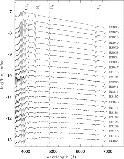
Observed SEDs of the 24 BSs in our sample. The spectra are roughly ordered in a temperature sequence, decreasing from top to bottom. Vertical dotted lines indicate the loci of four major spectral features, H 6562 Å, H
 4860 Å, H
 4340 Å and Ca K 3933 Å.
Qualitatively, the spectra in Fig. 1 are roughly ordered as a temperature sequence, based on visual inspection of the slope of the SED. It is interesting to note that the sequence of Balmer features, distinguishable down to H11 ( Å), from bottom to top, exhibits an increase up to BS025, indicating that BS005 should have a temperature compatible with that expected for a late B star. Similarly, the Ca K line at 3933 Å is nearly absent in the two hottest objects and steadily increases in strength, overcoming the intensity of the blend with Hε and the Ca H line at 3968 Å at the position of BS184. Another interesting feature easily observable in the spectra is the CH G band at 4300 Å. This feature is strongest for the two objects at the bottom. Again, from bottom to top, this feature disappears at the position of BS093. Therefore, this star should correspond roughly to spectral type A5 (about Teff= 8000 K).
We apply an absolute-flux calibration using intermediate-band photometric data (resembling spectrophotometric observations) collected at an earlier time (Deng et al. 1999). In brief, the 24 BSs were observed photometrically using the Beijing–Arizona–Taipei–Connecticut (BATC) intermediate-band filters. These observations included 11 of the 15 filters in this system, covering a range from 3500 to 10 000 Å. The shortest wavelength covered by our data set was obtained using a filter centred on 3890 Å. By convolving the observed BS spectra with the six intermediate-band (b, d, f, g, h and i; central wavelengths at 3890, 4550, 5270, 5795, 6075 and 6660 Å, respectively) transmission curves, six new magnitudes for each object were derived. These magnitudes were compared with those obtained with the BATC photometric observations and permitted the derivation of the scaling factors to transform the spectroscopy-based magnitudes to the absolute BATC system. The accurate intermediate-band photometry in the BATC system secures (recalibrates) the overall shape of the observed spectra for all programme stars.
To assess the quality of the overall SED shapes and to check the precision of the calibration, the spectrophotometrically calibrated spectra were used to construct broad-band photometry, which can then be compared with standard broad-band observations. Two sets of V, (B−V) observations from Sandquist & Shetrone (2003)– who provided photometric data of BSs in M67 for a study of variability in the light curves – and Girard et al. (1989)– who studied the relative proper motions and the stellar velocity dispersion of M67 – are compared with the artificial magnitudes and colours (see Table 2) of the 24 BSs, derived by convolving the B and V filter-response functions with the calibrated spectra. Adopting a distance modulus of DM = 9.97 mag and a colour excess E(B−V) of 0.059 mag for M67 (taken from WEBDA1), the observations (both the location with respect to the cluster's MS turn-off and the magnitudes and colours of the programme stars) can very well be reproduced using the artificial CMD photometry, as shown in Fig. 2. The artificial photometry was also compared with direct broad-band photometry (magnitudes and colours). A perfect match was found, as shown in Fig. 3, in which the residuals in V magnitude, δV=V−Vthiswork, and (B−V) colour index δ(B−V) = (B−V) − (B−V)thiswork are displayed. No systematic differences were found, whereas the random difference between the data derived from our spectra and from direct photometry is compatible with observational errors of a few per cent of a magnitude. Fig. 3 independently shows that our spectral observations and calibration are accurate to a satisfactory degree.
Artificial colours and magnitudes of our sample BSs.
| Name | V |  |
| BS005 | 10.02 |  0.064 0.064 |
| BS018 | 10.68 | 0.083 |
| BS025 | 10.95 | 0.107 |
| BS029 | 10.93 | 0.200 |
| BS034 | 10.95 | 0.232 |
| BS038 | 11.10 | 0.190 |
| BS040 | 11.29 | 0.118 |
| BS043 | 10.94 | 0.437 |
| BS046 | 11.22 | 0.405 |
| BS047 | 11.34 | 0.301 |
| BS065 | 11.32 | 0.613 |
| BS093 | 12.27 | 0.247 |
| BS111 | 12.16 | 0.447 |
| BS115 | 12.33 | 0.375 |
| BS116 | 11.99 | 0.576 |
| BS126 | 12.22 | 0.492 |
| BS131 | 12.60 | 0.385 |
| BS139 | 12.28 | 0.538 |
| BS143 | 12.30 | 0.556 |
| BS182 | 12.71 | 0.474 |
| BS184 | 12.72 | 0.482 |
| BS185 | 12.82 | 0.423 |
| BS206 | 12.92 | 0.396 |
| BS216 | 12.92 | 0.430 |
| Name | V | |
| BS005 | 10.02 | 0.064 |
| BS018 | 10.68 | 0.083 |
| BS025 | 10.95 | 0.107 |
| BS029 | 10.93 | 0.200 |
| BS034 | 10.95 | 0.232 |
| BS038 | 11.10 | 0.190 |
| BS040 | 11.29 | 0.118 |
| BS043 | 10.94 | 0.437 |
| BS046 | 11.22 | 0.405 |
| BS047 | 11.34 | 0.301 |
| BS065 | 11.32 | 0.613 |
| BS093 | 12.27 | 0.247 |
| BS111 | 12.16 | 0.447 |
| BS115 | 12.33 | 0.375 |
| BS116 | 11.99 | 0.576 |
| BS126 | 12.22 | 0.492 |
| BS131 | 12.60 | 0.385 |
| BS139 | 12.28 | 0.538 |
| BS143 | 12.30 | 0.556 |
| BS182 | 12.71 | 0.474 |
| BS184 | 12.72 | 0.482 |
| BS185 | 12.82 | 0.423 |
| BS206 | 12.92 | 0.396 |
| BS216 | 12.92 | 0.430 |
Artificial colours and magnitudes of our sample BSs.
| Name | V | |
| BS005 | 10.02 | 0.064 |
| BS018 | 10.68 | 0.083 |
| BS025 | 10.95 | 0.107 |
| BS029 | 10.93 | 0.200 |
| BS034 | 10.95 | 0.232 |
| BS038 | 11.10 | 0.190 |
| BS040 | 11.29 | 0.118 |
| BS043 | 10.94 | 0.437 |
| BS046 | 11.22 | 0.405 |
| BS047 | 11.34 | 0.301 |
| BS065 | 11.32 | 0.613 |
| BS093 | 12.27 | 0.247 |
| BS111 | 12.16 | 0.447 |
| BS115 | 12.33 | 0.375 |
| BS116 | 11.99 | 0.576 |
| BS126 | 12.22 | 0.492 |
| BS131 | 12.60 | 0.385 |
| BS139 | 12.28 | 0.538 |
| BS143 | 12.30 | 0.556 |
| BS182 | 12.71 | 0.474 |
| BS184 | 12.72 | 0.482 |
| BS185 | 12.82 | 0.423 |
| BS206 | 12.92 | 0.396 |
| BS216 | 12.92 | 0.430 |
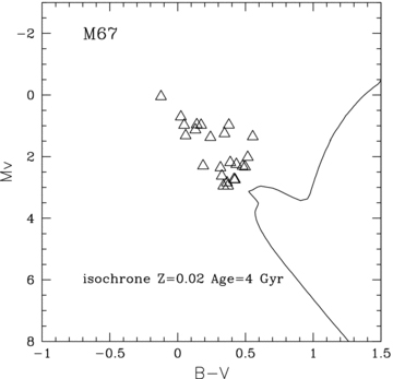
Artificial CMD for the BSs in M67. The full sample of 24 BSs is marked with open triangles. The solid line is the 4-Gyr isochrone of solar metallicity from Bertelli et al. (1994).
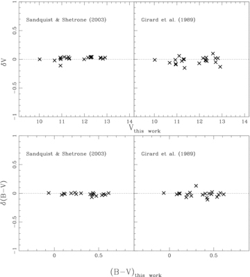
A comparison of visual magnitudes (top panels) and  colour indices (bottom panels) of our programme stars between the present paper and those of Sandquist & Shetrone (2003) and Girard et al. (1989).
3 SPECTRAL FITTING AND ANALYSIS
In order to study the spectral properties of BSs and to determine the effective temperature and surface gravity of our sample stars, we applied simple flux-fitting methods, using three different libraries of reference stellar spectra, both observed and synthetic. In all cases we assume a solar chemical composition for M67 stars, which is in agreement with observational determinations (Hobbs & Thorburn 1991; Bressan & Tautvais̃iene 1996).
Each calibrated spectrum was compared with every entry in the spectral atlas of Pickles (1998). The comparison was carried out after normalizing our spectra and those in the reference atlas to the flux at
 5556 Å. The algorithm we have implemented finds the spectrum (and its associated parameters) in the atlas that produces the minimum standard deviation, σ, of the residual flux,
  , computed for each λ.
Because of the marked decrease in sensitivity of the CCD at the shortest wavelengths, the spectral regime considered for the flux fitting excludes the region at
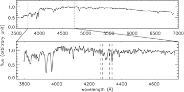
 Å. Fig. 4 displays the best fit and residuals for BS018 and BS126 (top panels). The solid and dashed lines are, respectively, the BSs' calibrated spectra and the best-fitting flux from the Pickles library. The labels at the top indicate the star ID, its temperature and spectral type designation.
A similar procedure was followed by using the spectral grids of Lejeune, Cuisinier & Buser (1997, 1998) which are, for the segment of the parameter space under consideration, mostly based on Kurucz (1993) low-resolution theoretical fluxes. In this case, both sets of spectra (BSs and model fluxes) were normalized to the flux at
 Å. A set of best-fitting parameters is found by directly comparing the observed spectra with each of the model fluxes. It is important to note that in this way, as well as in the previous point, the best fit always corresponds to a grid point. In Fig. 4 we show the best fit for the stars BS018 and BS126 (bottom panels). The solid and dashed lines are, respectively, the BSs' calibrated spectra and the best-fitting theoretical flux. The label on the right gives the parameters of the best-fitting model atmosphere.
In this case we made use of the bluered library (Bertone et al. 2003, 2008). bluered is a high-resolution (
 ) grid of over 800 synthetic stellar spectra, covering SEDs in the optical range (
 Å). The library is based on the atlas9 model atmospheres and has been computed with the synthe code developed by Kurucz (1993). The grid spans a large volume in the fundamental parameter space, accounting for virtually any stellar type from O to M stars and from dwarfs to supergiants. An important aspect of this grid, although of marginal relevance for the parameters associated with our programme stars, is that its calculation includes the effect of diatomic molecules, in particular TiO. A best-fitting spectrum was found in the two-dimensional space covering (
 ), after minimizing the statistical variance in the relative-flux domain as a measure of the similarity between target spectrum and theoretical SEDs across bluered (Bertone et al. 2004). As in the comparisons above, we have assumed a solar chemical composition for M67. It is worth noting that the grid of theoretical spectra has been properly modified to simulate the instrumental set-up. The results are shown in columns (6) and (7) of Table 3, whereas contour plots for BS018 and BS126 are shown in Fig. 5.
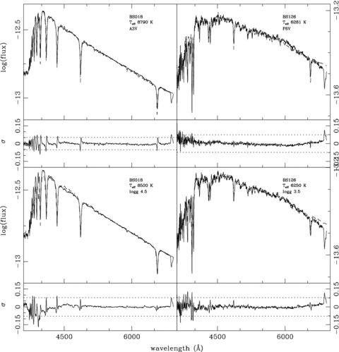
Best fits for two representative BSs, BS018 and BS126. The solid and dashed lines show, respectively, the observed spectra and the best-fitting Pickles (top panels) and Kurucz low-resolution spectra (bottom panels). The smaller panels below each spectrum correspond to the residuals, as explained in the text, and the dotted lines indicate the 3σ boundaries.
Best-fitting parameters.
| Namea | BATC-Pickles | BATC-Lejeune | BATC-bluered |  | |||
| Teff (K) | Spectral type | Teff (K) |  (dex) (dex) | Teff (K) |  (dex) (dex) | ||
| BS005 | 12 589 | B6IV | 12 625 | 5.00 | 11 050 | 3.1 | 977 |
| BS018 | 8790 | A3V | 8500 | 4.50 | 8500 | 4.0 | 1434 |
| BS025 | 8492 | A5V | 8500 | 4.25 | 8950 | 5.0 | 1066 |
| BS029c | 8054 | A7V | 7813 | 4.38 | 8100 | 5.0 | 1267 |
| BS034c | 8054 | A7III | 7688 | 4.38 | 7900 | 5.0 | 1284 |
| BS038 | 8054 | A7III | 7750 | 4.00 | 8050 | 5.0 | 1263 |
| BS040 | 8790 | A3V | 8625 | 4.75 | 8450 | 4.2 | 968 |
| BS043c | 6469 | F5V | 6500 | 3.50 | 6700 | 4.7 | 975 |
| BS046c | 6776 | F2V | 6625 | 3.88 | 6850 | 4.7 | 1082 |
| BS047c | 7586 | F0III | 7250 | 4.00 | 7500 | 4.8 | 752 |
| BS065 | 5636 | G2V | 5750 | 3.50 | 6000 | 4.2 | 1072 |
| BS093 | 7586 | F0III | 7625 | 4.25 | 7800 | 5.0 | 1280 |
| BS111c | 6281 | F6V | 6500 | 3.50 | 6600 | 4.6 | 997 |
| BS115c | 6776 | F2V | 7000 | 4.25 | 7050 | 4.7 | 1195 |
| BS116 | 6039 | F8V | 5938 | 3.75 | 6150 | 4.5 | 792 |
| BS126 | 6281 | F6V | 6250 | 3.50 | 6450 | 4.8 | 277 |
| BS131 | 6776 | F2V | 6875 | 4.75 | 6950 | 4.7 | 1273 |
| BS139 | 6039 | F8V | 6000 | 3.50 | 6200 | 4.6 | 984 |
| BS143 | 6039 | F8V | 6000 | 3.50 | 6100 | 4.1 | 1005 |
| BS182 | 6281 | F6V | 6250 | 4.00 | 6500 | 4.7 | 751 |
| BS184c | 6281 | F6V | 6375 | 4.25 | 6500 | 4.6 | 1036 |
| BS185 | 6531 | F5V | 6438 | 4.00 | 6700 | 4.7 | 145 |
| BS206 | 6776 | F2V | 6750 | 4.50 | 6900 | 4.7 | 2204 |
| BS216 | 6531 | F5V | 6500 | 4.50 | 6700 | 4.7 | 2226 |
| Namea | BATC-Pickles | BATC-Lejeune | BATC-bluered | | |||
| Teff (K) | Spectral type | Teff (K) | (dex) | Teff (K) | (dex) | ||
| BS005 | 12 589 | B6IV | 12 625 | 5.00 | 11 050 | 3.1 | 977 |
| BS018 | 8790 | A3V | 8500 | 4.50 | 8500 | 4.0 | 1434 |
| BS025 | 8492 | A5V | 8500 | 4.25 | 8950 | 5.0 | 1066 |
| BS029c | 8054 | A7V | 7813 | 4.38 | 8100 | 5.0 | 1267 |
| BS034c | 8054 | A7III | 7688 | 4.38 | 7900 | 5.0 | 1284 |
| BS038 | 8054 | A7III | 7750 | 4.00 | 8050 | 5.0 | 1263 |
| BS040 | 8790 | A3V | 8625 | 4.75 | 8450 | 4.2 | 968 |
| BS043c | 6469 | F5V | 6500 | 3.50 | 6700 | 4.7 | 975 |
| BS046c | 6776 | F2V | 6625 | 3.88 | 6850 | 4.7 | 1082 |
| BS047c | 7586 | F0III | 7250 | 4.00 | 7500 | 4.8 | 752 |
| BS065 | 5636 | G2V | 5750 | 3.50 | 6000 | 4.2 | 1072 |
| BS093 | 7586 | F0III | 7625 | 4.25 | 7800 | 5.0 | 1280 |
| BS111c | 6281 | F6V | 6500 | 3.50 | 6600 | 4.6 | 997 |
| BS115c | 6776 | F2V | 7000 | 4.25 | 7050 | 4.7 | 1195 |
| BS116 | 6039 | F8V | 5938 | 3.75 | 6150 | 4.5 | 792 |
| BS126 | 6281 | F6V | 6250 | 3.50 | 6450 | 4.8 | 277 |
| BS131 | 6776 | F2V | 6875 | 4.75 | 6950 | 4.7 | 1273 |
| BS139 | 6039 | F8V | 6000 | 3.50 | 6200 | 4.6 | 984 |
| BS143 | 6039 | F8V | 6000 | 3.50 | 6100 | 4.1 | 1005 |
| BS182 | 6281 | F6V | 6250 | 4.00 | 6500 | 4.7 | 751 |
| BS184c | 6281 | F6V | 6375 | 4.25 | 6500 | 4.6 | 1036 |
| BS185 | 6531 | F5V | 6438 | 4.00 | 6700 | 4.7 | 145 |
| BS206 | 6776 | F2V | 6750 | 4.50 | 6900 | 4.7 | 2204 |
| BS216 | 6531 | F5V | 6500 | 4.50 | 6700 | 4.7 | 2226 |
a Stellar identification from Fan et al. (1996); bsanders number (Sanders 1977); cbinary population.
Best-fitting parameters.
| Namea | BATC-Pickles | BATC-Lejeune | BATC-bluered | | |||
| Teff (K) | Spectral type | Teff (K) | (dex) | Teff (K) | (dex) | ||
| BS005 | 12 589 | B6IV | 12 625 | 5.00 | 11 050 | 3.1 | 977 |
| BS018 | 8790 | A3V | 8500 | 4.50 | 8500 | 4.0 | 1434 |
| BS025 | 8492 | A5V | 8500 | 4.25 | 8950 | 5.0 | 1066 |
| BS029c | 8054 | A7V | 7813 | 4.38 | 8100 | 5.0 | 1267 |
| BS034c | 8054 | A7III | 7688 | 4.38 | 7900 | 5.0 | 1284 |
| BS038 | 8054 | A7III | 7750 | 4.00 | 8050 | 5.0 | 1263 |
| BS040 | 8790 | A3V | 8625 | 4.75 | 8450 | 4.2 | 968 |
| BS043c | 6469 | F5V | 6500 | 3.50 | 6700 | 4.7 | 975 |
| BS046c | 6776 | F2V | 6625 | 3.88 | 6850 | 4.7 | 1082 |
| BS047c | 7586 | F0III | 7250 | 4.00 | 7500 | 4.8 | 752 |
| BS065 | 5636 | G2V | 5750 | 3.50 | 6000 | 4.2 | 1072 |
| BS093 | 7586 | F0III | 7625 | 4.25 | 7800 | 5.0 | 1280 |
| BS111c | 6281 | F6V | 6500 | 3.50 | 6600 | 4.6 | 997 |
| BS115c | 6776 | F2V | 7000 | 4.25 | 7050 | 4.7 | 1195 |
| BS116 | 6039 | F8V | 5938 | 3.75 | 6150 | 4.5 | 792 |
| BS126 | 6281 | F6V | 6250 | 3.50 | 6450 | 4.8 | 277 |
| BS131 | 6776 | F2V | 6875 | 4.75 | 6950 | 4.7 | 1273 |
| BS139 | 6039 | F8V | 6000 | 3.50 | 6200 | 4.6 | 984 |
| BS143 | 6039 | F8V | 6000 | 3.50 | 6100 | 4.1 | 1005 |
| BS182 | 6281 | F6V | 6250 | 4.00 | 6500 | 4.7 | 751 |
| BS184c | 6281 | F6V | 6375 | 4.25 | 6500 | 4.6 | 1036 |
| BS185 | 6531 | F5V | 6438 | 4.00 | 6700 | 4.7 | 145 |
| BS206 | 6776 | F2V | 6750 | 4.50 | 6900 | 4.7 | 2204 |
| BS216 | 6531 | F5V | 6500 | 4.50 | 6700 | 4.7 | 2226 |
a Stellar identification from Fan et al. (1996); bsanders number (Sanders 1977); cbinary population.
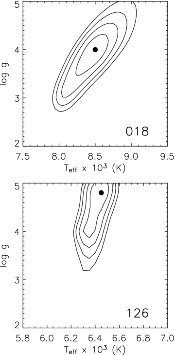
Contour plots for BS018 (top panel) and BS126 (bottom panel). The solid dot corresponds to the best parameter estimate; the contour levels indicate the 1, 2, 3 and 4σ uncertainties.
The results from the three methods are listed in Table 3, where columns (1)–(8) include, respectively, the object ID, the parameter pairs ( or spectral type) and the identification numbers following Sanders (1977), for ease of cross-identification.
The agreement among the effective temperature estimates provided by the three methods is on the order of 2–6 per cent and, in general, the best-fitting Teff values based on the bluered library are the highest, apart from the case of the hottest star, BS005, where the best fit is about 1550 K lower. The discrepancy in this case arises from the associated low log g value, which is about 2 dex lower than the corresponding result from the Lejeune library, since the flux-fitting method, applied to intermediate-resolution spectra, is affected by a  degeneracy, where a lower surface gravity implies a cooler temperature (Buzzoni et al. 2001).
A larger discrepancy affects the derived surface gravities of our sample stars, for which the highest values are most often provided by the bluered library. These latter results are, however, affected by an average 1σ error of  dex (see Fig. 5.) The systematically higher parameter values of the bluered spectra can be understood as in Bertone et al. (2008), who show that the Teff and log g values that are obtained from comparing the Sun with the bluered spectra (at very high spectral resolution) are a few per cent higher than those commonly accepted because the physical parameters of the absorption lines included in the spectral synthesis generate deeper features – which are counterbalanced by raising both the effective temperature and the surface gravity. In general, the current determinations of gravity for the programme stars are limited by the low resolution.
4 FINE-TUNING OF THE GRAVITY DETERMINATION
Complementary to the analysis presented in the previous section, we obtained observations at OAGH of the BS sample with an alternative set-up that allows, in principle, the separation of potentially fiducial gravity indicators. In particular, we will make use of the indicators defined by Rose (1984, 1994), which consist of line ratios of several pairs of features and the corresponding index–index diagnostic diagrams, and the hydrogen-absorption indices defined by Worthey et al. (1994) as part of the Lick system. These two approaches are necessary in view of the large effective temperature interval covered by the BSs.
New observations were carried out on 2008 February 24–27 using the Boller & Chivens spectrograph and the Versarray  1300 CCD detector optimized for the blue spectral interval. We used the
  mm−1 grating and a slit width of
  m, which yielded a nominal dispersion of 0.7 Å pixel−1 and a resolution of 2.6 Å FWHM. The grating was positioned to obtain spectra in the interval 3800–4700 Å where all of the gravity indicators cited above are defined.
The sample consisted of two stellar sets. The first corresponds to the full sample of BSs, whereas the other contains nearly 50 objects that served as gravity templates. The latter set was selected from the catalogues of Cayrel de Strobel et al. (1997); Cayrel de Strobel, Soubiran & Ralite (2001). Data reduction up to the standard flux calibration was performed using the conventional procedures of iraf and utilizing a set of standard stars observed each night. We considered it very important to secure calibrated fluxes to provide reproducible results when analysing data collected with other instruments. In Table 4 we list the control sample, showing in columns (1)–(5) the stellar identification, the spectral type and the associated stellar parameters collected from Cayrel de Strobel et al. (1997, 2001). For the stars with multiple determinations we provide the average values.
Stars used as gravity templates.
| Name | Spectral type | Teff (K) |  (dex) (dex) | [Fe/H] (dex) |
| HD025621 | F6IV | 6251 | 3.95 | 0.01 |
| HD027962 | A2IV | 9000 | 4.00 | 0.40 |
| HD028271 | F7V | 6160 | 3.85 |  0.10 0.10 |
| HD028978 | A2V | 9164 | 3.70 | 0.14 |
| HD031295 | A0V | 8860 | 4.12 |  1.08 1.08 |
| HD032537 | F0V | 6904 | 4.00 |  0.30 0.30 |
| HD033256 | F2V | 6219 | 3.94 |  0.31 0.31 |
| HD033608 | F5V | 6526 | 4.09 | 0.23 |
| HD033959 | A9IV | 7670 | 3.55 | 0.00 |
| HD034578 | A5II | 8300 | 1.85 | 0.16 |
| HD035497 | B7III | 13 622 | 3.80 |  0.10 0.10 |
| HD035984 | F6III | 6175 | 3.68 |  0.07 0.07 |
| HD038899 | B9IV | 10 903 | 4.00 | 0.01 |
| HD043386 | F5IV-V | 6480 | 4.27 |  0.06 0.06 |
| HD061295 | F6II | 6925 | 3.00 | 0.25 |
| HD076292 | F3III | 6866 | 3.77 |  0.22 0.22 |
| HD085235 | A3IV | 11 200 | 3.55 |  0.40 0.40 |
| HD087822 | F4V | 6597 | 4.10 | 0.17 |
| HD091752 | F3V | 6352 | 3.94 |  0.27 0.27 |
| HD094028 | F4V | 5960 | 4.23 |  1.46 1.46 |
| HD095418 | A1V | 9953 | 4.10 | 0.47 |
| HD097633 | A2V | 9395 | 3.57 | 0.04 |
| HD099028 | F4IV | 6739 | 3.98 | 0.06 |
| HD099285 | F2V | 6599 | 3.84 |  0.22 0.22 |
| HD100563 | F5V | 6401 | 4.31 | 0.05 |
| HD101606 | F4V | 6105 | 4.10 |  0.78 0.78 |
| HD102574 | F7V | 6030 | 3.92 | 0.16 |
| HD110411 | A0V | 8970 | 4.36 |  1.00 1.00 |
| HD117361 | F0IV | 6789 | 3.95 |  0.27 0.27 |
| HD120136 | F6IV | 6430 | 4.19 | 0.25 |
| HD126660 | F7V | 6338 | 4.29 |  0.05 0.05 |
| HD128167 | F2V | 6708 | 4.32 |  0.38 0.38 |
| HD130945 | F7IV | 6431 | 4.06 | 0.06 |
| HD132375 | F8V | 6344 | 4.25 |  0.05 0.05 |
| HD134083 | F5V | 6632 | 4.50 | 0.10 |
| HD136064 | F9IV | 6140 | 4.02 |  0.05 0.05 |
| HD137052 | F5IV | 6385 | 3.91 |  0.12 0.12 |
| HD139457 | F8V | 5941 | 4.06 |  0.52 0.52 |
| HD142357 | F5II-III | 6450 | 3.30 | 0.20 |
| HD142860 | F6IV | 6280 | 4.10 |  0.18 0.18 |
| HD144206 | B9III | 11 833 | 3.67 | 0.01 |
| HD144284 | F8IV | 6309 | 4.13 | 0.20 |
| HD145976 | F3V | 6720 | 4.10 | 0.01 |
| HD150012 | F5IV | 6380 | 3.80 | 0.05 |
| HD155646 | F5IV | 6179 | 3.92 |  0.14 0.14 |
| HD157373 | F4V | 6420 | 4.07 |  0.48 0.48 |
| HD157856 | F3V | 6309 | 3.93 |  0.18 0.18 |
| HD159332 | F6V | 6184 | 3.85 |  0.23 0.23 |
| HD161149 | F5II | 6600 | 2.95 | 0.55 |
| Name | Spectral type | Teff (K) | (dex) | [Fe/H] (dex) |
| HD025621 | F6IV | 6251 | 3.95 | 0.01 |
| HD027962 | A2IV | 9000 | 4.00 | 0.40 |
| HD028271 | F7V | 6160 | 3.85 | 0.10 |
| HD028978 | A2V | 9164 | 3.70 | 0.14 |
| HD031295 | A0V | 8860 | 4.12 | 1.08 |
| HD032537 | F0V | 6904 | 4.00 | 0.30 |
| HD033256 | F2V | 6219 | 3.94 | 0.31 |
| HD033608 | F5V | 6526 | 4.09 | 0.23 |
| HD033959 | A9IV | 7670 | 3.55 | 0.00 |
| HD034578 | A5II | 8300 | 1.85 | 0.16 |
| HD035497 | B7III | 13 622 | 3.80 | 0.10 |
| HD035984 | F6III | 6175 | 3.68 | 0.07 |
| HD038899 | B9IV | 10 903 | 4.00 | 0.01 |
| HD043386 | F5IV-V | 6480 | 4.27 | 0.06 |
| HD061295 | F6II | 6925 | 3.00 | 0.25 |
| HD076292 | F3III | 6866 | 3.77 | 0.22 |
| HD085235 | A3IV | 11 200 | 3.55 | 0.40 |
| HD087822 | F4V | 6597 | 4.10 | 0.17 |
| HD091752 | F3V | 6352 | 3.94 | 0.27 |
| HD094028 | F4V | 5960 | 4.23 | 1.46 |
| HD095418 | A1V | 9953 | 4.10 | 0.47 |
| HD097633 | A2V | 9395 | 3.57 | 0.04 |
| HD099028 | F4IV | 6739 | 3.98 | 0.06 |
| HD099285 | F2V | 6599 | 3.84 | 0.22 |
| HD100563 | F5V | 6401 | 4.31 | 0.05 |
| HD101606 | F4V | 6105 | 4.10 | 0.78 |
| HD102574 | F7V | 6030 | 3.92 | 0.16 |
| HD110411 | A0V | 8970 | 4.36 | 1.00 |
| HD117361 | F0IV | 6789 | 3.95 | 0.27 |
| HD120136 | F6IV | 6430 | 4.19 | 0.25 |
| HD126660 | F7V | 6338 | 4.29 | 0.05 |
| HD128167 | F2V | 6708 | 4.32 | 0.38 |
| HD130945 | F7IV | 6431 | 4.06 | 0.06 |
| HD132375 | F8V | 6344 | 4.25 | 0.05 |
| HD134083 | F5V | 6632 | 4.50 | 0.10 |
| HD136064 | F9IV | 6140 | 4.02 | 0.05 |
| HD137052 | F5IV | 6385 | 3.91 | 0.12 |
| HD139457 | F8V | 5941 | 4.06 | 0.52 |
| HD142357 | F5II-III | 6450 | 3.30 | 0.20 |
| HD142860 | F6IV | 6280 | 4.10 | 0.18 |
| HD144206 | B9III | 11 833 | 3.67 | 0.01 |
| HD144284 | F8IV | 6309 | 4.13 | 0.20 |
| HD145976 | F3V | 6720 | 4.10 | 0.01 |
| HD150012 | F5IV | 6380 | 3.80 | 0.05 |
| HD155646 | F5IV | 6179 | 3.92 | 0.14 |
| HD157373 | F4V | 6420 | 4.07 | 0.48 |
| HD157856 | F3V | 6309 | 3.93 | 0.18 |
| HD159332 | F6V | 6184 | 3.85 | 0.23 |
| HD161149 | F5II | 6600 | 2.95 | 0.55 |
Stars used as gravity templates.
| Name | Spectral type | Teff (K) | (dex) | [Fe/H] (dex) |
| HD025621 | F6IV | 6251 | 3.95 | 0.01 |
| HD027962 | A2IV | 9000 | 4.00 | 0.40 |
| HD028271 | F7V | 6160 | 3.85 | 0.10 |
| HD028978 | A2V | 9164 | 3.70 | 0.14 |
| HD031295 | A0V | 8860 | 4.12 | 1.08 |
| HD032537 | F0V | 6904 | 4.00 | 0.30 |
| HD033256 | F2V | 6219 | 3.94 | 0.31 |
| HD033608 | F5V | 6526 | 4.09 | 0.23 |
| HD033959 | A9IV | 7670 | 3.55 | 0.00 |
| HD034578 | A5II | 8300 | 1.85 | 0.16 |
| HD035497 | B7III | 13 622 | 3.80 | 0.10 |
| HD035984 | F6III | 6175 | 3.68 | 0.07 |
| HD038899 | B9IV | 10 903 | 4.00 | 0.01 |
| HD043386 | F5IV-V | 6480 | 4.27 | 0.06 |
| HD061295 | F6II | 6925 | 3.00 | 0.25 |
| HD076292 | F3III | 6866 | 3.77 | 0.22 |
| HD085235 | A3IV | 11 200 | 3.55 | 0.40 |
| HD087822 | F4V | 6597 | 4.10 | 0.17 |
| HD091752 | F3V | 6352 | 3.94 | 0.27 |
| HD094028 | F4V | 5960 | 4.23 | 1.46 |
| HD095418 | A1V | 9953 | 4.10 | 0.47 |
| HD097633 | A2V | 9395 | 3.57 | 0.04 |
| HD099028 | F4IV | 6739 | 3.98 | 0.06 |
| HD099285 | F2V | 6599 | 3.84 | 0.22 |
| HD100563 | F5V | 6401 | 4.31 | 0.05 |
| HD101606 | F4V | 6105 | 4.10 | 0.78 |
| HD102574 | F7V | 6030 | 3.92 | 0.16 |
| HD110411 | A0V | 8970 | 4.36 | 1.00 |
| HD117361 | F0IV | 6789 | 3.95 | 0.27 |
| HD120136 | F6IV | 6430 | 4.19 | 0.25 |
| HD126660 | F7V | 6338 | 4.29 | 0.05 |
| HD128167 | F2V | 6708 | 4.32 | 0.38 |
| HD130945 | F7IV | 6431 | 4.06 | 0.06 |
| HD132375 | F8V | 6344 | 4.25 | 0.05 |
| HD134083 | F5V | 6632 | 4.50 | 0.10 |
| HD136064 | F9IV | 6140 | 4.02 | 0.05 |
| HD137052 | F5IV | 6385 | 3.91 | 0.12 |
| HD139457 | F8V | 5941 | 4.06 | 0.52 |
| HD142357 | F5II-III | 6450 | 3.30 | 0.20 |
| HD142860 | F6IV | 6280 | 4.10 | 0.18 |
| HD144206 | B9III | 11 833 | 3.67 | 0.01 |
| HD144284 | F8IV | 6309 | 4.13 | 0.20 |
| HD145976 | F3V | 6720 | 4.10 | 0.01 |
| HD150012 | F5IV | 6380 | 3.80 | 0.05 |
| HD155646 | F5IV | 6179 | 3.92 | 0.14 |
| HD157373 | F4V | 6420 | 4.07 | 0.48 |
| HD157856 | F3V | 6309 | 3.93 | 0.18 |
| HD159332 | F6V | 6184 | 3.85 | 0.23 |
| HD161149 | F5II | 6600 | 2.95 | 0.55 |
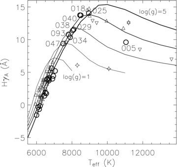
As an example of the flux-calibrated spectra we display, in Fig. 6, the lower resolution spectra of BS065 and a zoomed-in region at higher resolution. The vertical dashed lines indicate the position of several of the features used as gravity indicators, as described below.
Low-resolution (top panel) and intermediate-resolution (bottom panel) spectra of BS065. The dotted vertical lines indicate the positions of the Rose (1994) features used to define the gravity-sensitive line-depth index used in this paper.
4.1 The wavelength sequence, line ratios and Lick-like indices
We explored all possible combinations of the indices defined by Rose (1994), which are in the form of flux ratios at the central wavelengths of absorption lines or at pseudo-continuum loci, and the Lick/IDS indices (e.g. Worthey et al. 1994; Trager et al. 1998). We visually inspected the spectra of the template stars in search of additional pairs of features that could display a trend with gravity. At the end of the process, the indices that emerged as best gravity diagnostics are (1) the combination 4289/4271 versus Hγ/4325 from Rose's indices, for stars with  and (2) the Lick index
  , for stars hotter than 8000 K.
4.2 Analysis of line-depth ratios
As an important preliminary step, we theoretically verified the sensitivity of all of Rose's spectral features to surface gravity, in particular those that he identified as discriminators of gravity.
In spite of the similar spectral resolutions, this verification process is needed because Rose's spectra were not flux calibrated and, therefore, subject to effects inherent to the particular instrumental set-up he used. In other words, we have corroborated that the selected indices indeed separate the effects of effective temperature from those of gravity.
We calculated the line-depth ratios in a subsample of solar chemical composition synthetic spectra of bluered, after properly degrading the grid to match the working resolution of 2.6 Å. As mentioned previously, after exploring the full set of line ratios, we identified the diagnostic diagram including 4289/4271 versus Hγ/4325 as the best fiducial combination for differentiating amongst stellar luminosity classes.
Once we have confirmed their sensitivity to gravity, the next step is to transform the theoretical indices to our observational system. For this calibration we compare the theoretical indices with those measured from observed spectra. Note that theoretical values were obtained from bluered spectra after linearly interpolating the set of parameters of the template stars (Table 4). As an example of this comparison we show in Fig. 7 the correlations between the theoretical and the empirical indices for Hγ/4325 and H . This figure indicates that a linear transformation of the form
  suffices to properly match the theoretical and empirical indices.
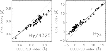
Comparisons between the theoretical and empirical indices for the sample of template stars. The empty circle in the right-hand panel corresponds to an object deviating more than 3σ. This object was not taken into account for the calibration. The dotted lines show the one-to-one correlations whereas the solid lines denote the best fits.
The comparison resulted in the transformation coefficients listed in Table 5, along with the rms error.
Linear transformation parameters.
| Index | a | b | rms |
| 4289/4271 | 0.385 | 0.605 | 0.017 |
| Hγ/4325 | 0.120 | 0.713 | 0.026 |
H | 2.21 | 0.80 | 0.74 |
| Index | a | b | rms |
| 4289/4271 | 0.385 | 0.605 | 0.017 |
| Hγ/4325 | 0.120 | 0.713 | 0.026 |
| H | 2.21 | 0.80 | 0.74 |
Linear transformation parameters.
| Index | a | b | rms |
| 4289/4271 | 0.385 | 0.605 | 0.017 |
| Hγ/4325 | 0.120 | 0.713 | 0.026 |
| H | 2.21 | 0.80 | 0.74 |
| Index | a | b | rms |
| 4289/4271 | 0.385 | 0.605 | 0.017 |
| Hγ/4325 | 0.120 | 0.713 | 0.026 |
| H | 2.21 | 0.80 | 0.74 |
In Fig. 8 we display the theoretical diagram (for solar metallicity) for a set of different effective temperatures and gravities, after application of the transformation described above. The dashed and solid lines illustrate, respectively, the iso-Teff and isogravity curves. In the top panel we overplot the loci of the template stars with  [Fe/H]
 dex. In the bottom panel we show the same diagram and the positions of the BSs.
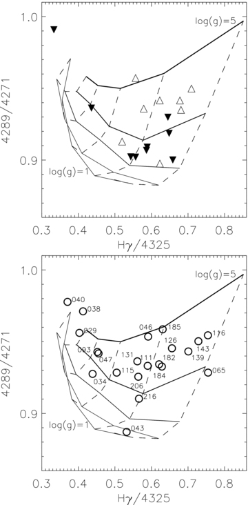
Diagnostic diagram for Rose's indices 4289/4271 versus H /4325. Dashed lines indicate the iso-Teff curves at 6000, 6500, 7000, 7500, 8000 and 8500 K (from right- to left-hand side), while the solid lines show isogravity trends at
  , 4, 3, 2 and 1 dex for the theoretically calculated indices. In the top panel the upward and downward triangles indicate, respectively, reference stars with gravities in the intervals
  4.5 dex and
  dex. In the bottom panel the positions of the BSs are marked with open circles, along with their identifications.
From inspection of the panels in Fig. 8 we note the following characteristics: up to an effective temperature of 7500 K, the indices can clearly be used to separate among stars of the three higher gravity bins, a sensitivity which appears enhanced for dwarfs and subgiants. Most of the BSs show up in the interval  . The only exceptions are BS034, BS043, BS065 and BS216, for which their loci in the diagrams indicate gravities lower than
  dex. Interestingly, in the work of Mathys (1991) two of these stars, BS034 and BS043, also turned out to be the lowest gravity objects, with
  and 3.44, respectively, although the latter star might require a more detailed analysis since it is part of a close pair (Girard et al. 1989).
Importantly, we note at this point that we have not (yet) attempted to use these diagrams to derive values for the atmospheric parameters, but instead we only provide an overall assessment of the gravity of the objects. For a more quantitative evaluation, a detailed analysis regarding the adequacy of the model spectra is necessary and still beyond the scope of the present paper. At any rate, it is important to mention that in spite of the potential problems associated with theoretical spectra (see Bertone et al. 2008) the diagrams clearly exhibit (even without prior knowledge of the atmospheric parameters) that most stars with  have surface gravities compatible with stars on the MS.
4.3 The Hγ Lick-like index
For the BS stars of higher temperatures we have measured absorption indices of the hydrogen Balmer lines, as defined by Trager et al. (1998). We have termed these indices ‘Lick-like’ since they have not been transformed to the Lick system. The overall behaviour of the indices associated with the Hγ and Hδ lines in empirical data has demonstrated that the indices barely depend on metallicity and are very sensitive to gravity for stars with  . We have constructed a theoretical diagnostic diagram of H
 versus Teff using bluered. In a similar fashion to the line-depth indices, we have calibrated theoretical indices by comparing them to the indices measured in the template stars. The results are included in Table 5. In Fig. 9 we display the theoretical trends for solar chemical composition, with the stars represented as in Fig. 8. In Fig. 9 we include the full sample of template stars regardless of their chemical composition. Note that the index values degenerate at low temperatures, whereas stars are well separated at high temperatures, in particular BS005 (our hottest object). According to this diagram, the three hottest stars have surface gravities in excess of
  , although – because of their temperature – their loci in the diagram do not allow us to precisely establish this parameter. The hot object BS005 appears to have a gravity of about
  , which is compatible with our determination using the bluered grid.
Lick-like index H as a function of effective temperature. The solid lines show the theoretical isogravity curves from
  to 1 dex from solar metallicity spectra. Observed stars are marked with the same symbols as in Fig. 8 with the addition of squares marking objects with log
  dex and starred symbols denoting stars with log
  dex.
dex.
There are two objects, BS029 and BS038, which do not lie within the physically expected regions in the two diagrams. For these stars, Mathys (1991) determined effective temperatures consistent with our determination, and gravities of  and 4.14 for BS029 and BS038, respectively.
Therefore, the spectral properties of BSs can be represented by MS stars with the same photometric properties when modelling a simple stellar population based on (photometric) observations of star clusters.
5 COMPARISON WITH PREVIOUS WORK
Previous studies of BSs in M67 include, for instance, Bruntt et al. (2007) for BS018, BS025, BS034, BS038, BS040, BS047 and BS093, based on asteroseismic analysis for δ Scuti pulsations, and Shetrone & Sandquist (2000) for BS043, BS046, BS139 and BS206, based on abundance analysis. Mathys (1991) analysed 11 BSs in M67 and studies on binarity are also available (see below). However, a homogeneous survey of the full sample of BSs in M67 and complete atmospheric parameter determinations have not yet been carried out. Mathys (1991) presented a spectroscopic study of 11 BSs in M67, and performed a detailed abundance analysis for F 153 and F 185. He concluded that the effective temperatures and surface gravities of the BSs in M67 were quite similar to those of normal MS stars of the same spectral type.
There is an obvious difference between his method and ours. Based on the photometric data from Mermilliod (1988), Mathys (1991) derived the atmospheric parameters from the photometric measurements of the BSs in the Strömgren system, applying the relevant calibration to determine the effective temperatures and surface gravities of B-, A- and F-type stars using  photometry (Moon & Dworetsky 1985).
The effective temperatures derived from this paper (from bluered) for the 11 BSs in common are consistent with Mathys (1991), as shown in Fig. 10(a), and the surface-gravity determinations are less conclusive for most of the BSs compared with Mathys (1991), as shown in Fig. 10(b). The error bars (horizontal axes) in Fig. 10 were obtained based on bluered spectral fits, whereas the vertical error bars are from Mathys (1991).
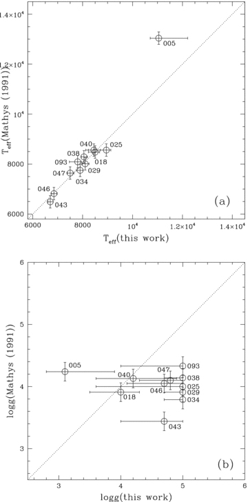
Comparison between our results and those of Mathys (1991): (a) effective temperature; (b) surface gravity. The dotted lines are the one-to-one correlations. The open circles are the 11 BSs (labelled by star IDs) in common between this paper and Mathys (1991).
For the 11 BSs in common, the surface gravities of BS005, BS018, BS025, BS038, BS040, BS046, BS047 and BS093 in both papers are in fairly good agreement, considering the error bars. Large deviations in surface gravities are found for the remaining three BSs in common (BS029, BS034, BS043), as shown in Fig. 10(b). Very likely, the undoubted binary nature of these three objects is responsible for the deviations between the two methods.
Indeed, there are eight objects in the list of BSs in M67 which are likely binary candidates, based on previous observations. The BSs identified as binaries are marked by asterisks in Table 3. The BS BS034 (S1284), for instance, is thought to be a binary system in the final stages of mass transfer (Milone & Latham 1992; Zhang, Zhang & Li 2005). Milone & Latham (1992) considered the dominant light contributor in BS034 to be the original primary (now the secondary) with an orbital period of 4.182 84 d and an eccentricity of  . Based on high-precision radial velocity measurements, they obtained a spectroscopic orbital solution for the BS binary system. They supposed that the mass transfer began fairly recently and that this BS was formed through stable mass transfer with nearly 100 per cent efficiency. BS046 (S1082) was found to be a complex unusual eclipsing binary system, or even a triple system of which the SED could be explained by the sum of a close binary and another MS star (van den Berg et al. 2001; Zhang et al. 2005). BS029 (S1267), BS043 (S975), BS047 (S752), BS111 (S997) and BS115 (S1195) were all identified as spectroscopic binaries with long periods ranging from 800 to 5000 d (Latham & Milone 1996). BS184 (S1036) was detected as a W UMa-type binary with a small amplitude of light variations, and a strong but stable O'Connell effect (Sandquist & Shetrone 2003).
In this paper, these binaries were easily fitted using model spectra of single stars. Although we cannot corroborate their binary nature, to within the limited resolution of the observations, we can nevertheless provide constraints on the BSs' spectral properties.
6 SUMMARY AND DISCUSSION
This study represents the first attempt to derive the parameters of the full sample of BSs in the old Galactic open cluster M67 (NGC 2682) in a homogeneous way. Low-resolution spectra of the sample of 24 BSs in M67 were collected using the 2.12-m telescope of the Guillermo Haro Observatory (Mexico). The entire data set was recalibrated using the BATC intermediate-band photometric system, in addition to the usual relative calibration using standard stars, and was subsequently used for a comparison with three different stellar data bases aimed at studying their spectral properties in a systematic way. We found that all objects have gravity values in agreement with the expected values for objects in the hydrogen-burning stage.
Considering the original goal of our paper, we conclude that, in terms of spectroscopic properties at low resolution, the BSs can indeed be represented by empirical or theoretical data of (or compatible with) MS stars, at least in a low-density environment as in M67.
As a natural extension to this, it is further concluded that when building up the empirical SEDs of SSPs based on stellar clusters, the contributions due to BSs can be accounted for using photometry and stellar spectral libraries. This conclusion holds at least at low and intermediate spectral resolution.
Limited by the spectral resolution of the current observational data set, it is not possible to assess binarity and the formation mechanism of the sample of BSs in M67. We anticipate that a detailed chemical abundance analysis at high resolution will show signatures of these dynamical and physical processes. Therefore, the current work serves as a valuable starting point.
We thank the anonymous referee for rapid and useful comments. We would like to thank the National Science Foundation of China (NSFC) for support through grants 10573022, and the Ministry of Science and Technology of China through grant 2007CB815406. MC and EB would like to thank CONACYT through grants SEP-2005-49231 and SEP-2004-47904. We would like to thank Richard de Grijs for language proof reading the paper.
REFERENCES
