‘Orphan’ afterglows in the Universal structured jet model for γ-ray bursts Free

Abstract

1 INTRODUCTION

Surveys for transient sources may detect γ-ray burst (GRB) afterglows. In this paper, we call an ‘orphan’ afterglow any afterglow associated with such serendipitous searches, as opposed to ‘triggered’ GRB afterglows, localized through the preceding prompt γ-ray emission. Rhodes (1997) suggested that these surveys could be used to put constraints on the geometrical beaming angle of the GRB jets in the ‘top-hat’ (TH) model. In this model, GRBs are assumed to be uniformly emitting within a cone of angle θ_jet with sharp edges, where the luminosity drops suddenly to an undetectable level.

The suggestion by Rhodes (1997) is based on the fact that the prompt γ-ray emission is relativistically beamed within an angle θ_jet+ 1/Γ, where 1/Γ≪θ_jet. Thus, if the line of sight lies outside this angle, the GRB is unlikely to be detected. However, as the outflow slows down in the afterglow phase, the visible region increases to eventually encompass the observer's line of sight. At late times, Γ∼ 1 and the emission are roughly isotropic. This behaviour would suggest that more long-wavelength transients than γ-ray ones may be expected. Detections of transients at different wavelengths may thus be used to constrain the beaming factor of b∝θ⁻²_jet. A measure of this quantity would be of great importance as it would allow one to calibrate θ_jet and then estimate the true GRB rates (∝b) and energetics (∝b⁻¹).

Searches for OAs have been performed at various wavelengths, but none of them has yielded a firm detection. Several authors have used observations in the radio band to constrain the GRB rate and energetics (e.g. Perna & Loeb 1998; Woods & Loeb 1999; Paczyński 2001; Levinson et al. 2002; Gal-Yam et al. 2006), since late time (i.e. nearly isotropic) afterglow emission peaks in this band. The simplest and most common assumption is that the predicted number of OAs in a snapshot observation is proportional to the beaming factor. Perna & Loeb (1998) used the lack of detections to set an upper limit of b≲ 10³. More recently, Levinson et al. (2002) and Gal-Yam et al. (2006) compared their data with a more detailed model for radio afterglows. They showed that the number of expected OAs in a flux-limited survey is inversely proportional to b and they place a lower limit of b≳ 60.

X-ray survey data have been used to search for OAs by Grindlay (1999) and Greiner et al. (2000), while optical searches have been more numerous (Schaefer 2002; Vanden Berk et al. 2002; Becker et al. 2004; Rykoff et al. 2005; Rau, Greiner & Schwarz 2006; Malacrino et al. 2007a). Using shorter wavelengths than radio to constrain the beaming factor necessarily requires a careful comparison with theoretical predictions (e.g. Nakar, Piran & Granot 2002, hereafter N02; Totani & Panaitescu 2002, hereafter TP02), since the emission is likely to be still relativistically beamed when OAs are detected in those bands. Malacrino et al. (2007a,b) put the tightest optical constraints so far (see their fig. 3). Their non-detection resulted in an upper limit for the number of OAs on the sky that is marginally consistent with the predictions of TP02 and consistent with N02 and (hereafter Z07 Zou, Wu & Dai 2007).

The purpose of this paper is to predict results for searches of afterglows in surveys, for a different GRB jet structure. Currently, OA surveys generally aim at constraining the jet angle. However, if GRB outflows are not geometrically beamed but they rather have an anisotropic luminosity distribution, the interpretation of data within the TH scenario would be misleading.

Numerical simulations of collapsing massive stars (e.g. MacFadyen & Woosley 1999) show that the jet emerges from the star with an energy distribution E(θ) and Lorentz factor Γ(θ) that vary as a function of the angle θ from the jet axis. It has been shown (Rossi, Lazzati & Rees 2002; Zhang & Mészáros 2002) that, if E(θ) ∝θ⁻² the diversity of afterglow light curves can be ascribed to different viewing angles within the context of an universal structured jet (USJ). In the USJ model, the outflow is geometrically wide. In this paper, we will postulate that for each GRB two simultaneous and opposite jets with θ_jet= 90° are produced. In this model b= 1. The feature of having emission into 4π solid angle is attractive since it can explain the lack of OA detections, while the non-uniform energy distribution allows one to avoid the huge energy requirement, demanded by GRBs with an isotropic equivalent energy ≳10⁵⁴ erg (e.g. GRB 990123). An important consequence of the energy distribution law E(θ) ∝θ⁻² is that it establishes a unique relation between the viewing angle and the observed luminosity, once a radiation efficiency law with an angle is assumed. Thus, unlike in the TH model, the observed luminosity function is not a free parameter. Consequently, the uncertainties in the predicted OA rates in the USJ scenario are smaller than in the TH model (see Section 4).

In this paper, we use the USJ framework to compute the expected number of transients in an all-sky snapshot and their rate as a function of the survey sensitivity. The aim is pursued by the means of Monte Carlo simulations of the afterglow properties, as observed by X-ray, optical and radio surveys. The procedure is described in Section 2. We show prospects for OA detections with current and future surveys in Section 3. This allows us to identify the best survey characteristics to increase the chance of detection and single out the most promising future missions. A comparison of our results with the TH predictions is performed in Section 4. Finally, we discuss and conclude our work in Section 5.

Throughout the paper, we assume a flat Universe with and Ω_Λ= 0.7.

2 SIMULATING THE POPULATION OF ORPHAN AFTERGLOWS

We use Monte Carlo methods to simulate the population of GRB orphan afterglows in the USJ. GRBs are randomly generated on the sky with a probability distribution in redshift that traces the star formation rate (SFR) (Section 2.1). We use the external shock model to compute the afterglow luminosity curve (Section 2.2). The probability function for the viewing angle θ is given by the fraction of the solid angle associated with that angle, P(θ) ∝ sin (θ). Our simulation yields for radio, optical and X-ray bands the distribution of afterglow fluxes and the total number of afterglows on the sky for a snapshot observation, together with the average time T_th that an afterglow remains detectable in the sky, as a function of the detection threshold. Finally, we compute the OA detection rate for any flux-limited survey where the observation time is much greater than T_th.

2.1 Formation rate and γ-ray luminosity function

We assume that the GRB population in the universe is described by a redshift independent luminosity function, a redshift distribution and a distribution of the spectral parameters.

In the USJ, the isotropic equivalent kinetic energy in the afterglow phase has the angular dependence:

1

where the bright central spine with angular size θ_c has a maximum kinetic energy E_c=E(0). The expected luminosity function follows from (Rossi et al. 2002),

2

where L (erg s⁻¹) is the isotropic equivalent bolometric peak luminosity and L_c is proportional to E_c (see equation 4). In equation (2), we assume that the γ-ray emission efficiency and the ratio of mean luminosity to peak luminosity is independent of the angle.

The GRB comoving rate R_GRB(z) (yr⁻¹ Mpc⁻³) is assumed to follow the comoving rate R_SN(z) (yr⁻¹ Mpc⁻³) of type II supernovae R_GRB(z) =k×R_SN(z), where k≡R_GRB/R_SN is a free parameter of the model. We assume that these arise from the stars with masses above 8 M_⊙ and that the initial mass function has a Salpeter form (e.g. Porciani & Madau 2001). Daigne, Rossi & Mochkovitch (2006 hereafter DRM06) found that the above prescription is dubious for redshift greater than 2. However, most of the OAs that are detected in a survey are located at lower redshifts, where this assumption appears to hold. In our analysis, we find, in fact, that the mean OA redshift for any reasonable flux threshold is never greater than z= 2. The SFR we adopt to derive R_SN (dubbed SFR₂) and its comparison with data (Hopkins 2004) are shown in fig. 1 of DRM06. This SFR saturates beyond z∼ 2 at a level of 0.2 M_⊙ yr⁻¹Mpc⁻³. Even though this behaviour is consistent with data at the 1σ level, the flat extrapolation of our SFR after the peak remains questionable, since high-z data are plagued by uncertainty on the amount of dust extinction. However, as discussed above, we do not expect that uncertainties in the high-z behaviour of R_GRB(z) appreciably affect our results. The GRB redshift probability function is thus given by

3

where the comoving volume equals

and D_L(z) is the standard luminosity distance.

The spectral properties of GRBs are described by the distribution of their peak energy E_p and their low- and high-energy slopes α and β. For the peak energy, we assume a lognormal distribution with a mean value E_p,0 and a dispersion 0.3 dex. For the slopes, we adopt the observed distribution by Preece et al. (2000).

With these assumptions, the GRB population is entirely described by four free parameters: L_c and θ_c for the luminosity function, k for the comoving rate and E_p,0 for the spectral properties. Following the method described in DRM06, we constrained them by fitting simultaneously: (i) the log N − log P distribution of GRBs [where P(ph cm⁻² s⁻¹) is the peak flux] detected by the Burst and Transient Source experiment (BATSE; Kommers et al. 2000; Stern et al. 2000; Stern, Atteia & Hurley 2002); (ii) the peak energy distribution of bright BATSE bursts (Preece et al. 2000) and (iii) the HETE2 fraction of X-ray rich GRBs and X-ray flashes (Sakamoto et al. 2005). For a given set of parameters (L_c, θ_c, k, E_p,0), a population of ∼10⁵ GRBs is randomly generated, with a redshift z, a luminosity L and a spectrum characterized by a peak energy E_p and a low- and high-energy slope α and β. The four free parameters are then adjusted to minimize the χ² obtained when comparing the simulated data with the three observations listed above. More details about the procedure can be found in DRM06. The results for the best fit are log [L_c(erg s⁻¹)]= 53.7 ± 0.6 and for the luminosity function, log (k) =−5.99 ± 0.06 for the comoving rate and log [E_p,0 (keV)]= 2.8 ± 0.1 for the spectrum. The reduced χ²= 1.53 for 37 degrees of freedom. We note here that DRM06, assuming a power-law luminosity function, found approximately −1.6 as the best-fitting value for the slope when this is free to vary, as opposed to the slope ∼−2 predicted by the USJ model (equation 2). However, an acceptable χ² is also obtained in our case.

2.2 Physical description of afterglow light curves

The afterglow emission is modelled as synchrotron radiation from a relativistic blast-wave propagating in a constant density external medium (e.g. Mészáros & Rees 1997). We ignore the contribution from the reverse shock, although it dominates the afterglow emission in the first few tens of seconds after the GRB (Sari & Piran 1999), since OA observations occur much later. For the same reason, our results are largely independent of the choice of the initial Lorentz factor (which we fix at Γ₀= 300), since the deceleration time is unlikely to exceed 10³ s (e.g. Panaitescu & Kumar 2000). Similar considerations of timing allow us to neglect the modelling of the early afterglow features (flares, plateau, etc., e.g. Nousek 2006), which are not reproduced by the standard external shock model.

The code we use for the calculation is described in Rossi et al. (2004). For each light curve, L_a(erg s⁻¹Hz⁻¹), the input parameters are: the angular distribution of kinetic energy, the viewing angle, the shock parameters, the external density and the rest-frame frequency.

The luminosity function parameters, L_c and θ_c, constrained by the prompt emission data (Section 2.1) allow us to determine the kinetic energy distribution within the jet (equation 1), since

4

Inspection of current data suggests that the proportionality constant is of the order of 1 s. The γ-ray efficiency η_γ that is inferred from modelling data in the standard external–internal shock scenario is rather high, between ∼50 and ∼90 per cent (Panaitescu & Kumar 2002). This uncertainty together with the 1σ range of L_c implies 10⁵²≲E_c erg ≲ 2 × 10⁵⁴. We adopt E_c= 1.3 × 10⁵³ erg. Since the core angle is not strongly constrained by prompt emission data (see Section 2.1), we adopt a value at the low end of the 1σ range, θ_c= 4°, to account for the observed breaks in the light curves on day time-scales. The external shock and density parameters are chosen from the ranges of values inferred from afterglow modelling (e.g. Panaitescu & Kumar 2001; Panaitescu 2005).1 The fraction of energy at the shock that goes into accelerated electrons and magnetic field is ε_e= 0.05 and ε_B= 0.005, respectively; the electrons are accelerated into a power law with exponent p= 2.2. The external number density is taken to be n= 1 cm⁻³. The whole set of parameters (E_c, θ_c, ε_e, ε_B, p and n) yield results consistent with the observed afterglow flux distributions (Berger et al. 2005). Our flux distributions are shown in Figs 1–3. In the right-hand panels, we plot the histogram of fluxes in a given band for all afterglows detected in a snapshot observation of the sky. In the left-hand panels, we show the flux histogram of the same afterglows evaluated at a common observed time. These latter distributions compare favourably with figs 4–6 of Berger et al. (2005).2

Figure 1

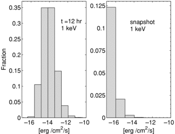
Flux distribution in the X-ray band at 1 keV energy; these distributions are intrinsic, i.e. no selection criteria have been applied. We choose the minimum flux, so that the arbitrary cut-off at 10 yr for the age of an afterglow in our simulations does not affect the shown distributions. Left-hand panel: the distribution of fluxes at 12 h after the trigger. This may be compared with fig. 5 of Berger et al. (2005), taking into account that their observed distribution suffers from selection effects. Right-hand panel: the flux distribution as it appears in a snapshot observation of the sky.

Open in new tabDownload slide

Figure 2

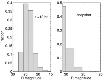
As Fig. 1 but for magnitude distributions in the R band. Our left-hand panel may be compared with fig. 4 of Berger et al. (2005).

Open in new tabDownload slide

Figure 3

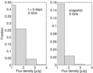
As Fig. 1 but for flux distributions in the radio band at 5 GHz frequency. Our left-hand panel may be compared with fig. 6 of Berger et al. (2005).

Open in new tabDownload slide

We compute afterglow light curves L_a[ν× (1 +z), θ, t′] for three observed frequencies, ν= 2.42 × 10¹⁷ Hz (1 keV), ν= 4 × 10¹⁴ Hz (R band) and ν= 5 × 10⁹ Hz; six redshifts, 0 ≤ z ≤ 20; 10 viewing angles, 0°≤θ≤ 90° and 57 comoving times t′, spanning 10 yr. We arrange those data in the form of a matrix that can be easily interpolated in order to assign a luminosity L_a to each simulated burst. The flux observed on the Earth is calculated from L_a with F=L_a(1 +z)/(4πD²_L). Examples of light curves are shown in Fig. 4: in this example, the GRB is situated at z= 1 and viewed under different angles, in our three bands of observation.

Figure 4

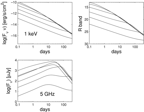
Afterglow light curves for a GRB at z= 1 in X-rays (upper left-hand panel), optical (upper right-hand panel) and radio (lower left-hand panel) bands. For each band, the different curves correspond to different viewing angles. From top to bottom panel, and 90°.

Open in new tabDownload slide

2.3 Monte Carlo code for ‘orphan’ afterglows

OAs are generated with a flat probability distribution in age, t_a (i.e. the time lag as observed on the Earth between the GRB explosion and the snapshot observation epoch), in an interval of 10 yr, at a rate of R_obs≃ 2195 yr⁻¹.3 For the sensitivities of interest in this paper, afterglows of 10 yr or older are undetectable. Their mean duration above threshold is indeed shorter than our total simulated time (see Figs 5–7). Therefore, the arbitrary cut-off at 10 yr does not influence our results.

Figure 5

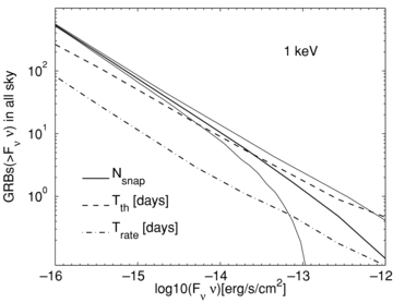
Expected number of afterglows in an all-sky snapshot observations in the X-ray band, as a function of the flux threshold (solid thick line). The thin solid lines are the 1σ contours. We also plot T_th (thick dashed line) and T_rate (thick dot–dashed line) in days.

Open in new tabDownload slide

Figure 6

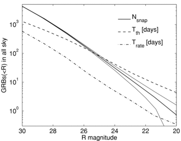
The same as Fig. 5, but for the R band.

Open in new tabDownload slide

Figure 7

The same as Fig. 5, but for the radio band.

Open in new tabDownload slide

We generate each GRB redshift, z, according to the probability distribution discussed in Section 2.1 and its viewing angle θ according to

5

with 0°≤θ≤ 90°. From the matrix of the afterglow luminosities interpolated at t_a/(1 +z), θ and ν(1 +z), we calculate the OA flux and compare it with a given flux threshold, F_th. We can, thus, compute the expected number of afterglows above F_th in a given band ν: N_snap(>F_th, ν). This is the number that would be seen in a snapshot observation of the entire sky.

Model predictions for a flux-limited survey require the calculations of two other quantities. First, the mean of the time interval t_th spent by an afterglow above the flux limit,

6

where we actually compute the geometric mean of t_th to avoid being biased by the extreme values. Secondly, the mean rate at which afterglows appear in the sky over the survey flux threshold,

7

We performed 160 simulations of flux-limited all-sky snapshots in radio and optical bands and 400 in X-rays, where we needed more statistic. We then computed the average N_snap, T_rate and T_th. The results are shown in Figs 5–7 (thick lines). They can be used to estimate the number of OAs expected in a given survey. If the observing time of a survey T_obs is shorter than the time T_th for which an afterglow is detectable, then we can consider it a snapshot observation and the total expected number of detected OAs is

8

where Ω_obs is the solid angle of the sky covered by the snapshot. Vice versa, the total expected number of OAs is computed as

9

3 RESULTS

Our results show that, as expected, the probability of detection and the mean duration above threshold increases with the survey sensitivity (Figs 5–7). A chance of detection in an all-sky snapshot (N_snap≳ 10) requires: a flux limit of νF_ν≲ 10⁻¹⁴ erg cm⁻² s⁻¹ at 1 keV; a limit magnitude of R≳ 23 in R band and a flux density threshold of F_ν≲ 1 mJy at 5 GHz.

3.1 Specific surveys predictions

In this section, we provide illustrative predictions for various current and planned surveys. We use here the results shown in Figs 5–7 and equations (8) and (9). We note that the following numbers should be taken as upper limits when compared with observations, since we did not consider detection limitations (e.g. host galaxy, dust absorption etc.) other than instrumental.

We also note that a detailed comparison between observation and theory requires knowledge of the specific survey strategies. However, generic conclusions can be drawn from the following examples.

3.2 X-rays

The two most sensitive X-ray surveys (∼1 × 10⁻¹⁵ erg s⁻¹ cm⁻² in the 0.5–2 keV band) performed by Chandra and XMM–Newton are the 2-Ms Chandra Deep Field-North and the 0.8-Ms XMM–Newton Lockman Hole field. They cover, respectively, an area of 0.13 and 0.43 deg². Since T_th≃ 52 d, these surveys are equivalent to two snapshot observations. The small coverage of the sky results in a very small detection probability of a few 10⁻⁴. Larger surveys, as the XMM–Newton Bright Serendipitous Source Sample (Della Ceca et al. 2004) or The Chandra Multi-wavelength Project (ChaMP; e.g. Kim et al. 2007), are less sensitive (νF_th≳ 10⁻¹⁴ erg s⁻¹ cm⁻²) and the increase in area is not sufficient to yield more than N_oa≲ 10⁻².

The ROSAT All-Sky Survey (RASS; e.g. Voges 1999) covers the full sky. The RASS exposure is 76 435 deg² d, with a sensitivity of 10⁻¹² erg s⁻¹ cm⁻². Therefore, the survey is equivalent to an all-sky observation with T_obs= 1.85 d. At this flux threshold, OAs are fast X-ray transients, lasting for T_th≃ 0.5 d and R_oa≃ 0.1 d⁻¹. Therefore, despite the large coverage of the sky, we predict that the survey should have found only N_oa≃ 0.2. Greiner et al. (2002) found 23 OA candidates. After spectroscopic follow-up, however, they concluded that most, if not all events, are stellar flares. This is in agreement with our predictions.

The prospects for detection are not exciting even for the future mission extended ROentgen Survey with an Imaging Telescope Array (eROSITA). It will perform the first imaging all-sky survey up to 10 keV with a sensitivity of 5.7 × 10⁻¹⁴ erg⁻¹ cm⁻² in the 0.5–2 keV band. We predict ∼2.3 OAs.

These dispiriting results can be understood from Figs 1 and 5: the flux limit should be ≲10⁻¹⁴ erg s⁻¹ cm⁻² in order to have a good chance of detection in one all-sky snapshot. To achieve such a sensitivity, a long exposure time is needed (e.g. ∼50 ksec for Chandra). Given the small field of view of the current instruments, a full sky scan is unfeasible. We conclude that X-ray surveys are a poor tool for OA searches if jets are described by the USJ model.

3.3 Optical

The most recent optical OA searches are the ones by Rau et al. (2006) and Malacrino et al. (2007a). Rau et al. observed 12 deg² of sky for 25 nights, separated by one or two nights. They used the MPI/European Southern Observatory (MPI/ESO) Telescope at La Silla, reaching R= 23. Since at that sensitivity T_th≃ 22 d and T_rate≃ 2 d, we compute the expected OAs through an average rate of R_oa= 6.3 d⁻¹. We find N_oa= 0.02, considering an actual observing time of 12.5 d. Malacrino et al. used images from the CFHTLS very wide survey. They searched 490 deg² down to R= 22.5. They observed 25–30 deg² every month over a period of two to three nights (Malacrino et al. 2006). Since T_th≃ 17 d, we can consider their survey a snapshot observation and we predict N_oa= 0.1. Recently, Malacrino et al. (2007b) have rejected the only candidate they had identified in their first work.

The most recent Sloan Digital Sky Survey (SDSS) data release (Adelman-McCarthy et al. 2007) includes imaging of 9583 deg², with a R magnitude limit of 22.2. We expect N_oa≃ 1.5. If we take a more conservative magnitude limit of 19 to account for the need for spectroscopic identification, the detection probability drops to ∼0.05.

The previous meagre results are due to the fact that a very large detection area is essential for these sensitivities (Fig. 2, right-hand panel and Fig. 6). Only with the flux limit of the Subaru Prime Focus Camera (R≃ 26 in 10 min of exposure), we could restrict ourselves to 5 per cent of the sky and get a snapshot with N_oa≃ 10. This, however, would require a total observing time of T_obs≃ 57 d.

Future larger surveys include GAIA (Perryman et al. 2001) and the Panoramic Survey Telescope and Rapid Response System (Pan-Starrs; e.g. Kaiser et al. 2002). The first is an all-sky survey with a magnitude limit of R∼ 20. It will observe each part of the sky 60 times separated by 1 m (Lattanzi et al. 2000). At this sensitivity, an OA stays in the sky on average for ∼3.8 d; thus, GAIA will perform 60 independent snapshots of the sky, with a prediction of N_oa≃ 44. Pan-STARRS is expected to scan three-quarters of the entire sky in about a week, down to an apparent magnitude of 24. Since T_th≃ 43 d, this can be considered a snapshot observation and we expect ≃ 23 OAs. Finally, the Large Synoptic Survey Telescope (LSST) is planned to cover 10 000 deg² every three nights down to a depth of R≃ 24.5 (Ivezic et al. 2008). This would yield ∼13 afterglows every three nights. Both Pan-STARR and LSST will be able to repeatedly observe an afterglow source, thus monitoring its variability and enhancing the chances of identification.

Thus, future optical surveys could be powerful tools for OA searches.

3.4 Radio

Levinson et al. (2002) searched for transients by comparing the Faint Images of the Radio Sky at Twenty-cm (FIRST) and NRAO VLA Sky Survey (NVSS) radio catalogues and found nine candidates. Gal-Yam et al. (2006) rejected all candidates by means of follow-up radio and optical observations and placed an upper limit (95 per cent confidence) of 65 radio transients for the entire sky above 6 mJy at 1.5 GHz. This may be translated to a sensitivity threshold of 3.3 mJy at 5 GHz, using a typical late-time spectral shape in radio of F∝ν^−0.5 (TP02). We predict ≃ 1.4 radio afterglows.

Recently, Bower et al. (2007) published an archival survey with data from the Very Large Array, spanning 22 yr. For an effective area of 10 deg², we get a rate of ≃4 × 10⁻²yr⁻¹ for OAs brighter than 370 μJy. This rate is too low to account for the 10 detected transients. In addition, the observed transient duration of approximately a week suggests that those sources are not indeed afterglows, which are expected to last above that threshold for approximately half a year.

Figs 3 and 7 and the above examples show that the OA search would greatly benefit from lowering the survey sensitivity below 1 mJy, with an area of ≳10 000 deg².

FIRST Becker, White & Helfand (1995) has covered over 10⁴deg² of the North Galactic Cap. The survey area has been chosen to coincide with that of the SDSS. The sensitivity is F_th∼ 1 mJy at 1.4 GHz. This may be translated into a flux limit of 0.5 mJy at 5 GHz. If we consider, as for the SDSS, an area of 9583 deg², we expect ≃7 OAs.

The plan is for the Allen Telescope Array (ATA)4 to observe 10⁴deg² at mJy sensitivity and later to go as deep as ∼0.1 mJy at 5 GHz. The expected number of OAs would then rise from a few to 50.

4 COMPARISON WITH THE ‘TOP-HAT’ MODEL

In Fig. 8, we compare our results for N_snap (solid line) with published predictions for the TH model in R band (dashed lines). From bottom to top panel, we plot the ‘standard’ model by Z07; the ‘preferred’ and the ‘optimistic’ models by N02 and the model by TP02. The curves from these works have similar slopes but they vary in normalization by several orders of magnitude. The main difference is the assumed afterglow luminosity function.

Figure 8

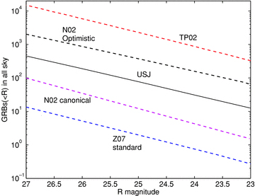
Comparison between the predicted number of OAs in the TH and USJ model in R band. From bottom to top panel, we plot for the TH model, the ‘standard’ model by Z07; the preferred and the optimistic models by N02 and the model by TP02. The solid line is the prediction of the USJ model.

Open in new tabDownload slide

This is the result of different choices for the opening angle and total jet energy distributions and the afterglow radiation efficiency. Z07 assume constant total (beamed corrected) energy E_tot= 10⁵¹ erg and a power-law distribution of opening angles P(θ_jet) ∝θ⁻¹_jet. N02 assume constant peak flux at θ_obs=θ_jet and a fixed average opening angle θ_jet= 0.1 rad (‘canonical’ model) and θ_jet= 0.05 rad (‘optimistic’ model). Finally, TP02 assume that the whole GRB population is represented by 10 well-studied events. We also note that within each model there is an order of magnitude uncertainty. For example, Zou et al. results differ by an order of magnitude between E_tot= 5 × 10⁵⁰ and 5 × 10⁵¹ erg (their fig. 4).

These uncertainties in the TH model are due to the fact that neither the opening angle distribution nor the total jet energy distribution is uniquely defined by the model or unbiasely determined by observations (e.g. through the observed luminosity function). The USJ model, instead, has more predictive power, since it has less degrees of freedom.

From the comparison in Fig. 8, one concludes that our model predictions fall roughly in the middle of the range of published results for the TH model. The differences in the predictions between our model and any individual TH model are large enough to be significant, but there is a sufficiently wide class of plausible TH models to encompass almost any luminosity function of OA that might be observed in the future. In principle, therefore, OA observations could rule out the USJ model (noting, of course, that there is a similar level of uncertainty to our predictions as individual TH models), but the same cannot be said for the TH model. The TH model could be tested by a combination of orphan afterglow observations and independent constraints on the parameters of the model.

5 DISCUSSION AND CONCLUSIONS

The realization that GRBs may be jetted has triggered studies of orphan afterglows. Early studies assumed that the prompt GRB emission comes from a sharp jet, in which case the ratio of afterglows to that of GRBs yields a constraint on the GRB beaming fraction (or equivalently the opening angle of the GRB jet). This parameter is of importance for a proper assessment of GRB rates and energetics.

The structured jet model has offered an equivalent explanation for afterglow phenomenology. However, its interpretation of the light curve breaks is different: they would arise from viewing angle effects and not from geometrical collimation. In fact, if GRB jets are indeed structured, most, if not all, afterglows should be generally preceded by a prompt emission pointing towards the observer. Therefore, even if, in practice, the relative number of detections in various bands depends on the survey strategy, the ratio should tend to unity (b= 1) if events are detectable at arbitrarily low fluxes.

In this paper, we have investigated the detection prospects of afterglows for flux-limited surveys, in the USJ framework. We conclude that large sky coverage is essential in all bands. In addition, X-ray and radio instruments should push their flux limit below 10⁻¹⁴ erg s⁻¹ cm⁻² (at 1 keV) and ∼1 mJy (at 5 GHz), respectively. Current and planned X-ray surveys are thus not suited for OAs searches, if the jet is structured. The FIRST and the future ATA projects could be successful in detecting radio OAs. The potential is even better for future optical all-sky surveys, such as GAIA and Pan-Starrs. We also note that it would be worthwhile to exploit the great sensitivity of the Suprime-Cam, for which 5–10 per cent of the whole sky is sufficient for positive detections. Certainly, a combination of X-ray, optical and radio observations would yield the most of information and will help understanding whether the USJ describes correctly the structure of the jet.

We are very grateful to T. Totani and A. Panaitescu for providing us with their data for the TH predictions. We also acknowledge very useful discussions with G. Bower and E. Nakar. EMR acknowledges support from NASA though Chandra Postdoctoral Fellowship grant number PF5-60040 awarded by the Chandra X-ray Center, which is operated by the Smithsonian Astrophysical Observatory for NASA under contract NASA8-03060.

REFERENCES

Author notes