Multisite campaign on the open cluster M67 – I. Observations and photometric reductions Free

Abstract

1 INTRODUCTION

Asteroseismology of stellar clusters is potentially a powerful tool. The assumption of a common age, distance and chemical composition provides stringent constraints on each cluster member, which significantly improves the asteroseismic output (Gough & Novotny 1993). Hence, detecting oscillations in cluster stars in a range of evolutionary states holds promise of providing new tests of stellar evolution theory. Driven by this great potential, several studies have been aimed at detecting solar-like oscillations in the open cluster M67 (Gilliland & Brown 1988; Gilliland et al. 1991, 1993; Gilliland & Brown 1992a) and in the globular cluster M4 (Frandsen et al., in preparation). The most ambitious campaign was reported by Gilliland et al. (1993), who used seven 2.5-m to 5-m class telescopes during one week in a global photometric network to target 11 turn-off stars in M67. Despite these efforts, they did not claim unambiguous detection of oscillations. However, one of their conclusions was that oscillations should be detectable in the more evolved red giant stars due to higher expected oscillation amplitudes. However, the oscillation periods of up to several hours and expected frequency separations of a few 10⁻⁶ Hz would require a time base of roughly one month on these stars. Recent month-long studies using single- or dual-site high-precision radial velocity measurements (σ∼ 2 m s⁻¹) on bright field stars have clearly demonstrated that solar-like oscillations are present in red giant stars (Frandsen et al. 2002; Barban et al. 2004; de Ridder et al. 2006). However, due to non-continuous coverage these data suffered badly from aliasing in the Fourier spectrum, which complicated the detailed frequency analysis. Multisite or space observations are therefore required (Stello et al. 2006). Such observations will hopefully soon become available for red giant stars in the field from the MOST, COROT and Kepler missions. However, after the cancellation of the ESA Eddington mission, no current or planned space project will measure stellar oscillations in cluster stars. Using high-precision spectrographs from ground to measure radial velocities in red giants is not possible due to the lack of a global network that can achieve high-precision velocities on an ensemble of relatively faint cluster stars. Hence, the only feasible approach is ground-based photometry.

In this investigation, we again target M67 using multisite photometric observations. Unlike the previous studies on this cluster, our primary targets are the red giant stars (see Fig. 1). Extrapolating the L/M-scaling relation (Kjeldsen & Bedding 1995) predicts the amplitude of these stars to be in the range 50–500 μmag. Although very low, these amplitudes are significantly higher than that for the turn-off stars targeted by, e.g. Gilliland et al. (1993). In addition to the red giants, more than 300 cluster stars were observed during the campaign. Many are high-amplitude variables such as W UMa systems, δ Scuti stars and eclipsing binaries, some of which are already known. This campaign provides a unique data set to investigate these stars as well (Bruntt et al., in preparation). With emphasis on the low-amplitude red giant stars, the main purpose of this paper is to describe the optimization of time series data towards achieving the highest possible signal-to-noise ratio in the Fourier spectrum (in amplitude). Further discussion on the extraction of p modes from the Fourier spectra of these stars will be presented by Stello et al. (in preparation).

Figure 1

Colour–magnitude diagram of the open cluster M67 (photometry by Montgomery, Marschall & Janes 1993). The red giant target stars are indicated with filled symbols. The numbers correspond to those indicated in Fig. 3. The solid line is an isochrone [(m−M) = 9.7  mag,   age = 4.0  Gyr,  Z= 0.0198 and Y= 0.2734] from the BaSTI data base (Pietrinferni et al. 2004).

Open in new tabDownload slide

2 OBSERVATIONS

We observed the open cluster M67 from 2004 January 6 to February 17 using nine telescopes (0.6-m to 2.1-m class) in a global multisite network. The sites were distributed in longitude to allow continuous time series photometry during the six-week observing programme. We were allocated 164 nights of telescope time which, due to bad weather, yielded about 100 clear nights (see Fig. 2 and Table 1). In the first 18 d we observed 34 per cent of the time and in the following three weeks the coverage was 80 per cent. For the entire campaign (43 d) the coverage was 56 per cent.

Figure 2

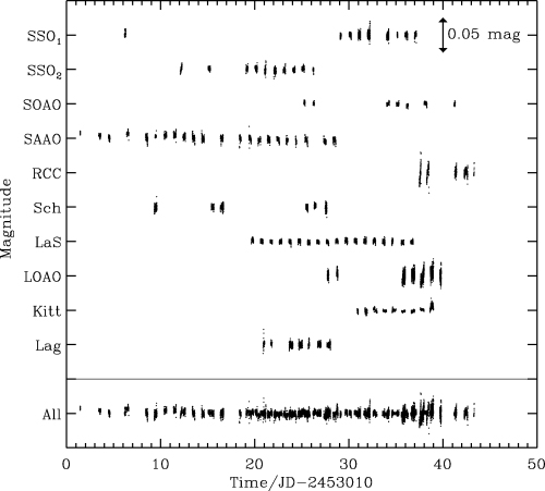
Time series of star no. 10 for all sites (after removing outliers and correcting for colour-dependent extinction; see Section 5.2). The site abbreviations are explained in Table 1.

Open in new tabDownload slide

The participating telescopes and detectors had different properties and the data sets are therefore rather diverse in terms of field of view (FOV), cadence and noise properties. A summary of the observations and the instrument characteristics for each site is given in Table 1. We indicate the smallest and largest FOV in Fig. 3. The red giant stars are indicated as well. Observations at each telescope were planned to optimize the signal-to-noise ratio for solar-like oscillations in the red giant stars. We did that by calculating both the noise and the expected oscillation amplitudes (the signal) in different photometric filters. The amplitudes were estimated from Kjeldsen & Bedding (1995, equation 5) and the noise was estimated by photon counting statistics. These calculations showed that the Johnson B and V filters were favourable, but an on-site test was required to establish which of these was superior at each telescope. The observers therefore chose filters based on an initial test at the beginning of the first night. All sites except Kitt Peak chose the V filter. No phase change is seen in the solar oscillations between observations obtained in different filters over the range 400–700 nm (Jiménez et al. 1999). We therefore expect the same adiabatic behaviour for high-order solar-like oscillations in other stars as well. Hence, combining data based on different filters can be done after a simple rescaling of the amplitude, and corresponding adjustment of the weights to preserve the signal-to-noise ratio.

Figure 3

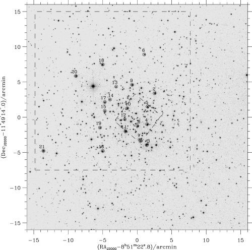
M67 FOV. SAAO with the smallest FOV and LOAO with the largest are indicated with dashed squares. The red giant stars are marked with circles. Source: STScI Digitized Sky Survey.

Open in new tabDownload slide

To obtain a noise level which was essentially limited by scintillation and photon noise, it was important to avoid drift on the CCD of the stellar field. The aim was to have each star confined within a few pixels. Not all sites had autoguiding systems and as a result we found very different drift characteristics from site to site (see Fig. 4). The images were defocused to obtain a higher duty cycle, but we avoided crowding.

Figure 4

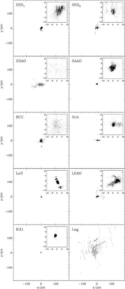
The position on the CCD of star no. 10 relative to a reference frame. The insets show the inner 20 by 20 pixels. Although autoguiding is good at LaS, instrument rotation introduced drift during the observing run for stars far from the rotation axis.

Open in new tabDownload slide

The exposure time at each site was adjusted to have star no. 4 just below the saturation limit, which provided a safety margin for the large group of clump stars that were 0.3-mag fainter (see Fig. 1). However, the two brighter stars (Nos 3 and 11) were therefore often saturated. Due to their expected long oscillation periods (Stello et al., in preparation), on time-scales similar to typical instrumental drift, the results on these stars were likely to provide only limited scientific output. Keeping these two stars above the saturation limit resulted in lower noise for the stars at the base of the red giant branch (stars 6, 13, 12 and 14) which were more likely to produce useful results.

3 CALIBRATION

We calibrated each CCD image using four steps:

• overscan subtraction (not all CCDs had an overscan region),

• subtraction of bias (the bias levels were stable enough to use a single master bias image for each CCD),

• correction for non-linearity (see Section 3.1),

• flat-fielding to correct for pixel-to-pixel variations in the quantum efficiency (we used one master flat-field for each CCD; for Kitt Peak and the RCC this was based on dome flats, while we used sky flats for all other sites).

We found that the dark current was negligible compared to the readout noise for all sites and it was therefore ignored. These four steps were standard except the non-linearity correction, which is described in more detail in the following section.

3.1 CCD linearity calibrations

In this project, a few target stars were relatively close to the CCD saturation limit, at flux levels for which the non-linear response of the CCD gain could be significant. It is important to correct for these gain variations to attain the high photometric precision required by this project.

Linearity at high flux levels was investigated for all CCDs using a ‘classical’ linearity test. We used an approach similar to that described by Gilliland et al. (1993). The method measures relative variations in the CCD amplifier gain, rather than absolute calibration in terms of e⁻/ADU. Flat-field images were taken sequentially with increasing exposure time, interleaved with reference images; e.g. 3 s, 10 s, 3 s, 10 s, … , 3 s, then followed by 3 s, 20 s, 3 s, 20 s, … , 3 s, until the final series, in which the longer exposures were almost saturated. The reference images allowed instabilities of the light source to be measured and removed. In some cases, however, the flat-field lamp varied on time-scales too short to be sampled and a correction could therefore not be made. The mean counts in the flat-field image, scaled according to the exposure time, were plotted versus the mean counts. Images with the same exposure time were grouped to form a single point, with an uncertainty equal to the group rms. In Fig. 5, we show the results of the linearity tests for all CCDs. Saturation occurred at 65 536 ADU except for the Schmidt, where it was at 16 384 ADU. From Fig. 5 (upper right-hand panel), we see that non-linearity can introduce variability in the stellar time series up to several per cent in non-photometric conditions (variable atmospheric transparency). Using ensemble photometry (Section 4) will, however, reduce this effect if the ensemble stars are roughly of equal colour and luminosity. We decided to correct for non-linearity for all sites except the Schmidt, which did not show measurable non-linear effects, and Laguna, where we only had measurements of the gain variations up to approximately 30 000 ADU, which was significantly lower than the intensity levels of most target stars. For LOAO, the data did not justify a description of the gain variation to be higher than a first-order polynomial fit, although a few points could indicate that higher-order features were present. The linearity calibration of the data from La Silla was based on a method described in Section 3.1.1, hence no fit was applied to the data shown in Fig. 5.

Figure 5

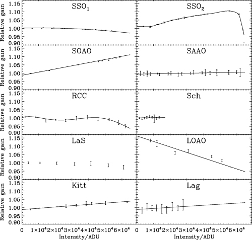
Classical linearity tests for all CCDs. For SSO₁, SSO₂ and SAAO, two separate tests have been merged. Error bars are plotted as 3 × rms to make them visible. The solid lines are polynomial fits used to correct the data for non-linearity.

Open in new tabDownload slide

We obtained calibration images at La Silla for a new and more elegant method for determining the linearity properties. This method provides a much more precise determination of the CCD gain variations, which we will compare with the classical method in the next section.

3.1.1 Ultrahigh precision method

The basic concept of the method described in this section was first outlined by Baldry (1999) and Knudsen (2000), and was developed into a fully applicable method by Stello (2002). Like the classical method, this method measures relative variations in the CCD amplifier gain using flat-field images of different exposure times, but it differs by using flat-fields that have a strong gradient e.g. by using a grism. Each flat-field showed a large smooth variation in light level from approximately the bias level to a significant fraction of the saturation limit, with the longest exposure reaching saturation (see Fig. 6). The advantage of this method is that the effect from instabilities in the light source used to obtain the flat-fields is very small, because we are sampling a large range (in the longest exposures the entire range) of the CCD gain response in a single exposure. The resulting measurement precision of the gain variations is several orders of magnitude better than the classical method. Further, this method requires relatively few images to achieve high precision, making it very efficient.

Figure 6

Linearity flat-field of the longest exposure, 410 s (see the text). The flat plateau at high row numbers is due to the digital saturation of the CCD.

Open in new tabDownload slide

We obtained spectral flats using the DFOSC spectrograph on the Danish 1.54-m telescope (La Silla). Light variation in one direction across the CCD was achieved using a grism to disperse the light from the slit illuminated by an internal telescope calibration lamp (Fig. 6). A series of images were acquired in the following way: 3 × 30 s, 3 × 130 s, 3 × 30 s, 3 × 250 s, 3 × 30 s, 3 × 370 s, 3 × 30 s, 3 × 390 s, 3 × 30 s, 3 × 410 s, 3 × 30 s. The control exposures of 30 s enabled long-term drift in the flat-field lamp to be removed. Although this improves the precision, it is not critical. After subtraction of overscan and bias, we corrected for the long-term drift of the flat-field lamp and made an average (master) flat-field for each exposure time. We then collapsed each master flat-field by averaging in one direction to obtain one-dimensional intensity curves, as shown in Fig. 7.

Figure 7

Two intensity curves of different exposure times, 410 s and 130 s (see the text). The flat part of the 410-s exposure at high row number is due to saturation of the CCD.

Open in new tabDownload slide

Due to non-linear effects in the CCD, the intensity we measure in the nth row is

1

where T_exp is the effective exposure time in seconds (after correcting for dead time of the shutter and short-term fluctuations in the light source), g(I(n)) is the CCD amplifier gain as a function of the measured intensity and S defines the shape of the intensity curves, hence S(n) expresses the intensity in the nth row from a 1-s exposure. Although the actual gain variations are a function of the received flux, we assume the CCD amplifier has a well-defined output signal for every input signal.

From two intensity curves with different exposure times, say 410 s and 130 s, we constructed the relative curve

2

where we have corrected for shutter dead time and verified that the shape S was stable. In Fig. 8 (top panel), we show the curve I_410s(n)/I_130s(n) versus I_410s(n), which we call a gain-ratio curve. At each intensity, I₁, this curve shows the gain ratio, g(I₁)/g(I₂), where I₂=I₁ 130 s/410  s. Thus, finding g(I) for any intensity level requires inversion of the gain-ratio curve in an iterative process.

Figure 8

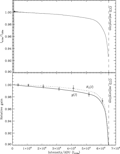
Top panel: gain-ratio curve based on two intensity curves of different exposure time (410 and 130 s). Bottom panel: inversion from smoothed gain-ratio curve R₁(I) (dotted) to final gain-curve g(I) (solid). For comparison, the measurements from the classical method (Fig. 5, LaS) and their error bars (1× rms) are indicated. The uncertainty on g(I) is of the order of 10 ppm. The smoothing of R₁(I) introduces a systematic error in g(I) of roughly 1 per cent near the saturation limit because the curve is steep.

Open in new tabDownload slide

We started out using a smoothed version of the measured gain-ratio curve, which we denoted R₁(I), as a first estimate for the actual underlying gain curve g(I) (see Fig. 8, bottom panel). Then, assuming g₁(I) =R₁(I), we computed a new gain-ratio curve, R₂(I) =g₁(I)/g₁(I  130 s/410 s) for all I. The new estimate for the gain was then corrected by the relative deviation between R₁ and R₂ according to g₂(I) = (R₁/R₂)g₁(I), etc. This iterative process stopped when R_i matched the measured R₁ and the corresponding g_i(I) was the desired gain curve. Before smoothing the measured gain-ratio curve (Fig. 8, top panel) we removed the noise at low intensities (0–1000 ADU) by replacing it with a linear fit to the data points from 1000 to 10 000 ADU. In the example shown, the gain-ratio curve is very similar to the final gain curve. However, this is not a feature of the method, but is due to the gain characteristics of the particular CCD amplifier. To ensure that all features in the gain were detected, we examined gain-ratio curves based on different exposure-time ratios. If a feature, say a bump in the CCD gain, is periodic for increasing intensity and hence repeated at all pairs of intensities (I₁, I₂) related as I₂=I₁  410 s/130 s, it will not show up in the gain-ratio curve based on 410 s and 130 s exposures (or any combination with the same exposure-time ratio). Our gain curves based on flat-fields with different exposure-time ratios, all showed an excellent match within the errors.

In Fig. 8 (bottom panel), we compare our new method with results from the classical method for La Silla (Fig. 5). The two methods are in agreement with each other, but the series of flat-field images for our new method is significantly faster to obtain, provides the relative gain for all intensities and has a precision more than 100 times better. However, it requires temporally stable but spatially variable illumination of the CCD (e.g. spectral flat-fields) which is not possible at every telescope.

4 ENSEMBLE PHOTOMETRY

The goal of this project is to measure relative light variations with very high precision. Hence, our approach is to obtain differential photometry taking advantage of the ensemble of stars in the FOV. Using an ensemble allows the effects from atmospheric variations, common to all stars, to be removed from the time series. The number of stars in the ensemble ranged from 116 (in the small FOV of SAAO) to 358 (for LOAO). We used the momf photometry package (Kjeldsen & Frandsen 1992) to extract the photometry from the reduced images. It calculates differential photometric time series by subtracting a reference time series which is a weighted average based on all ensemble stars. The weight given to each star is 1/rms³, which ensures that stars with a high rms in their time series, such as faint stars and high-amplitude variables, are strongly suppressed. momf was developed especially to produce time series photometry from large numbers of images (in particular defocused images) of semicrowded fields, similar to those obtained in this campaign. It combines point spread function (PSF) and aperture photometry. We chose 10 stars, not necessarily the same for each site, to define the shape of the PSF. These were all non-crowded bright stars, i.e. mostly red giant stars and a few bluer stars of the same luminosity (see Fig. 1). momf allows multiple apertures and calculates the total rms, σ_total, and the internal rms, σ_internal, of the time series based on each aperture. The first is just the rms of the time series while the latter is calculated as

3

where N is the number of points in the time series and m_i is the magnitude of the ith point in the series. For each site and each star we chose the aperture with the lowest σ_total in the time series.

5 IMPROVING THE PHOTOMETRY

5.1 Iterative sigma clipping

To improve the overall quality of the data, we first removed outliers. We calculated the point-to-point deviation of each data point, i, relative to its neighbouring points as

4

where m is the magnitude. We then removed data points, m_i, for which d_i > 3.0σ_i, where σ_i is the rms of d within a 3-h interval around data point i. This was done in an iterative loop until no more points were removed, which converged after a few iterations. We illustrate the underlying statistics of this process in Fig. 9, which shows that the cumulative distribution of d/σ has a significant non-white tail of deviating data points. Choosing the threshold is a trade-off between removing outliers and keeping statistically valid points. The threshold was chosen so that roughly 85 per cent of the removed points were real outliers and 15 per cent were valid points. We tested our sigma clipping method on generated random noise to verify that it was not too drastic in terms of removing extreme points from pure Gaussian noise. It removed less than 0.2 per cent, corresponding to about 35 points of the time series from the entire campaign. This should be compared to the approximately 250 data points removed in total from the real time series for each star. Results of the sigma clipping on the real data were further verified by visual inspection of diagrams similar to what is shown in Fig. 10.

Figure 9

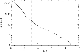
Cumulative distribution of d/σ (solid line) for the entire data set of star no. 10. The dotted line is an analytical Gaussian distribution for comparison, and the dashed line indicates the threshold for our sigma clipping process.

Open in new tabDownload slide

Figure 10

Photometric time series of star no. 10 for single nights from four sites. Outliers found by iterative sigma clipping are indicated with asterisks. The strong trend in the Kitt Peak data (curved time series) is due to colour-dependent extinction not removed by the ensemble normalization of momf. The corrected time series, has been shifted upwards by 0.02 mag for clarity (see Section 5.2).

Open in new tabDownload slide

5.2 Colour extinction

The data from Kitt Peak, which were the only ones obtained in the Johnson B filter, showed clear residual trends. This arises from an uncorrected wavelength dependence in the extinction (see Fig. 10). These trends were visible in the red giant stars because the reference time series calculated by momf was dominated by bluer stars. Decorrelating the differential photometry against airmass still left a lot of variation in the time series. Including more parameters, such as sky background, in the decorrelation process would affect the expected stellar signals significantly, which we verified with simulations. Subtracting a smoothed version of the individual time series was also too harsh on the stellar signal. Instead we tried using only the red giant stars themselves in the ensemble. For some targets this provided good results but for most it did not. Adding the much fainter main-sequence stars of similar colour to increase the sample size did not improve the results. We finally chose to correct the colour term from the momf differential photometry in a similar way to Gilliland & Brown (1988). For each image we fitted a linear relation to the target stars:

5

where m_k is the magnitude of star k, (B−V)_k is its colour and 〈m_k〉 is the average of the time series. To correct star j, we subtracted a fit that did not include the star itself

6

This was to prevent stellar signal being removed by the process, which we have confirmed with simulations. There were 12 red giant target stars with low noise levels, hence 11 stars were used in each fit, with a typical range of 1.00–1.25 mag in B−V colour. In Fig. 10 (bottom right-hand panel), we show the time series of one night of star no. 10 before and after correction of the colour term. The other sites showed weak effects from extinction, but these trends were not consistent from star to star or night by night, and the noise levels in the Fourier spectra did not improve if we performed the same correction as in the case of Kitt Peak. We therefore decided not to correct for residual extinction in the differential photometry at any other site.

5.3 Weight calculation

To be able to detect solar-like oscillations in the red giant stars, it is crucial that we obtain noise levels as low as possible in the frequency range where the oscillations are expected to appear in the Fourier spectra of the time series. It is known that weighting time series of inhomogeneous data can significantly improve the final signal-to-noise ratio level (Handler 2003). The important thing is that the final weights represent the true variance of the noise on time-scales similar to the stellar signal one wants to detect. We will use a weighting scheme similar to that used by Butler et al. (2004) and Kjeldsen et al. (2005) to minimize the noise in amplitude, which includes the following two steps.

• Calculate weights from the point-to-point variance (w_i= 1/σ²_i).

• Adjust the weights to obtain agreement between the noise at the relevant frequencies in the Fourier spectrum and the weights as being represented by w_i= 1/σ²_i.

• The point-to-point variance was not supplied by the photometric reduction package and these values had to be estimated from the local variance of the time series. We estimated the local scatter σ_i (=⁠) for each data point i as the rms of the d array (equation 4) using a moving boxcar. The width of the boxcar (5 h) was chosen to minimize the noise (in amplitude) in the weighted Fourier spectrum. The spectrum was calculated as a weighted discrete Fourier transform following the description of Frandsen et al. (1995). Having first removed outliers, we prevented good data from being down weighted by bad neighbouring points during this process.

• We then adjusted the weights night by night to be consistent with the noise level (in amplitude), σ_amp, between 300–900 μHz in the Fourier spectrum, requiring that (equation 3 in Butler et al. 2004). The idea is that noise in this frequency range would have components that affect the noise at slightly lower frequency as well where we expect the stellar signal to be for the red giant stars. Choosing a frequency range within the expected range of the stellar signal would effectively down-weight stellar signal, which is not desired.

In Fig. 11, we plot our final estimates of σ_i, including the adjustment multipliers for each night shown in the insets. The maximum adjustment was a factor of ∼2. For some sites, the noise in the final Fourier spectra in the range 300–900 μHz decreased by up to 20 per cent after adjusting weights on a night-by-night basis, but in most cases it was a 5–10 per cent decrease. We see that σ_i vary significantly during the observing run at many sites. For example, the range at Kitt Peak is 0.54–3.61 mmag (see Fig. 11).

Figure 11

Scatter for each site for star no. 10. The insets show the multiplication factor used to adjust σ_i for each night (see Section 5.3). The horizontal axes are the same as in the main panels.

Open in new tabDownload slide

6 ERROR BUDGET

To establish whether the noise in the final time series was at the irreducible lower limit dominated by photon noise and atmospheric scintillation, we estimated each noise component and compared with the measured noise in the time series in a similar way as in previous investigations by Gilliland & Brown (1988, 1992a) and Gilliland et al. (1993).

Our total error budget comprised scintillation and counting statistics within the aperture; the latter included stellar light, sky background, level in the flat-field, and CCD readout noise. The contribution from scintillation was estimated as

7

(Kjeldsen & Frandsen 1992, equation 3) using the factor of proportionality from Young (1967), D is the telescope diameter in centimetres, χ is the airmass, h is the elevation of the telescope in metres and T_exp is the exposure time in seconds per image. For the counting statistics, we used the expression from Kjeldsen & Frandsen (1992, equation 31):

8

where W is the full width at half-maximum of the stellar PSF in pixels, e_ff is the number of electrons per pixel in the flat-field, e_star is the number of electrons from the star within the aperture, r_AP is the radius in pixels of the aperture, e_sky is the number of electrons per pixel in the sky background and σ_RON is the CCD readout noise (per pixel) in electrons. Combining σ_scint and σ_count finally gives the estimated scatter

9

The estimated scatter was dominated by scintillation for the brighter stars and by photon noise for the fainter stars. The magnitude at which the noise changed from being scintillation dominated to photon noise dominated was in the range V= 10.5–12.0 mag but different from site to site. At a few sites, the contribution to the counting statistics from the flat-field was similar to the scintillation and hence significant for the brighter stars. In general, the readout noise and sky background could be neglected.

In Table 2, we give the measured internal scatter (equation 3) for each red giant star based on the full time series, which shows the overall quality of the data from star to star and from site to site. In general, star no. 10 had the lowest noise except for SAAO and LOAO. To compare with the estimated scatter (equation 9) we have, for each star and each site, measured the internal scatter (equation 3) for the best night, and the results are shown in Fig. 12. There are other sources of noise not included in our error budget, which can explain why some stars fall significantly above the line of proportionality. Saturation of the CCD will increase the noise significantly. For several sites, stars Nos 3, 4 and 11 were affected by saturation, which explains their higher noise levels. Close neighbouring stars can introduce higher noise in the photometry. Star no. 12 has three close neighbouring stars and at most sites it suffers from excess noise. If a star is located close to a bad column on the CCD the noise will also increase, which we see in some cases.

Figure 12

Measured scatter versus estimated scatter for the red giant stars. The measured scatter is σ_internal (equation 3) of the relative photometry based on the best night for each star. The estimated scatter is calculated from equation (9), which gives relative errors, and is scaled by a factor of 1.086 ppm/μmag to put it on the magnitude scale.

Open in new tabDownload slide

In summary, for stars that are not affected by crowding, saturation or bad columns, we generally see noise levels limited by photon and scintillation noise on the best nights. At one site (RCC) the noise is larger than estimated by a factor of 2, which is unexplained.

6.1 Noise comparison with previous campaigns

The first campaign aimed at detecting solar-like oscillations in M67 was carried out by Gilliland & Brown (1988), who used a 0.9-m telescope on two nights. Noise levels to ∼1.5 mmag per minute integration were attained for non-saturated stars (m_V≳ 12 mag). Later, Gilliland et al. (1991) observed M67 for two weeks from five sites using 0.6-m to 1.1-m class telescopes. The lowest rms in the time series of the non-saturated stars (m_V≳ 12.5) was 0.88 mmag per minute integration after high-pass filtering the data. For comparison, our best 0.6-m site (SOAO) showed an internal scatter (comparable to the rms of high-pass filtered data) down to ∼1.6 mmag per minute integration, and the best 1.0-m site (SAAO) showed ∼1.2 mmag per minute integration. A final, but direct, comparison can be made between our Kitt Peak observations of the red giant no. 10 with those obtained by Gilliland & Brown (1992a) using the same telescope in a similar campaign. Star no. 10 (no. 7 in Gilliland et al. 1991) was one of their targets with the lowest noise, which was 0.43 mmag per minute integration after high-pass filtering and decorrelating the data. In comparison, we obtained 0.50 mmag (based on the internal scatter, but without any high-pass filtering or decorrelation).

To summarize, we find noise levels as good as in previous studies based on similar size telescopes. However, this campaign has provided significantly longer time series (six weeks compared to a maximum of two weeks) with better coverage than earlier comparable campaigns, which implies lower noise levels in the final Fourier spectra.

6.2 Noise in the Fourier spectra

The noise levels in the Fourier spectra obtained by our weighting scheme were 20–30 μmag for the red giant stars that were not affected by excess noise from crowding, saturation or bad pixels. We therefore expect to be able to detect oscillations in the Fourier spectrum with ⁠. However, the detection threshold depends very much on the mode lifetime, which is unknown for these stars (Stello et al. 2006), and will require extensive simulations to quantify. This analysis will be published in a subsequent paper.

In Fig. 13, we show the Fourier spectrum of star no. 10, which is one of the best, to illustrate the noise level we have obtained. The noise level, indicated with the white line, is the average in the range 300–900 μHz. The detailed pulsation analysis of all red giants will be presented by Stello et al. (in preparation).

Figure 13

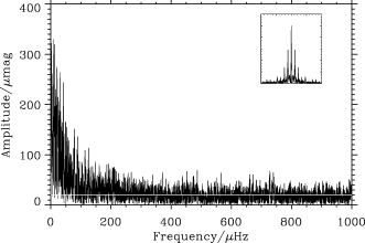
Fourier spectrum of star no. 10 (in amplitude). The white line indicates the noise level in the range 300–900 μHz. The inset shows the spectral window, which is on the same frequency scale as the main panel. Each data point has been weighted according to the weighting scheme described in Section 5.3.

Open in new tabDownload slide

7 CONCLUSIONS

We have collected 100 telescope nights of photometric multisite data of the open stellar cluster M67 over a six-week period. The focus of this paper was the discussion of our approach towards achieving the highest signal-to-noise ratio for the very low-amplitude (50–500 μmag) solar-like oscillations in the red giant stars. This included our careful reduction of the CCD images to obtain the lowest possible noise in the time series data, and our weighting scheme to reduce the noise level in the Fourier spectrum.

We have obtained a point-to-point scatter in the time series photometry down to about 1 mmag for most sites, while the largest participating telescope reached 0.5 mmag (Fig. 12). These values are similar to those from previous campaigns on M67 by Gilliland & Brown (1988), Gilliland et al. (1991) and Gilliland & Brown (1992b) which all used telescopes of similar size but for shorter time spans (maximum two weeks). Comparison of our best nights with known noise terms demonstrates that the attained point-to-point scatter is consistent with irreducible terms dominated by photon and scintillation noise for all sites but one (RCC), which shows extra noise of unknown origin (Fig. 12). With these scatter values, our weighting scheme provided a mean noise level in the Fourier spectra of approximately 20 μmag (in amplitude), which would allow us to detect solar-like oscillations in the red giant stars with assuming L/M-scaling.

This work was partly supported by the IAP P5/36 Interuniversity Attraction Poles Programme of the Belgian Federal Office of Scientific, Technical and Cultural Affairs. This paper uses observations made from the South African Astronomical Observatory (SAAO), Siding Spring Observatory (SSO) and the Danish 1.5-m telescope at ESO, La Silla, Chile. This research was supported by the Danish Natural Science Research Council through its centre for Ground-Based Observational Astronomy, IJAF.

REFERENCES