


Abstract
We obtain a robust, non-parametric, estimate of the Hubble constant from the linear diameters and rotation velocities of galaxies in the recent KLUN sample, calibrated using Cepheid distances to Hubble Space Telescope Key Project galaxies. There are two key features that make our analysis considerably more robust than previous work. First, the method is independent of the spatial distribution of galaxies and is insensitive to Malmquist bias. It may, therefore, be applied to more distant samples than so-called ‘plateau’ methods — making it much less vulnerable to the impact of peculiar motions in the Local Supercluster. Secondly, we include information on the galaxy rotation velocities in a fully non-parametric manner: unlike the conventional Tully–Fisher relation we reconstruct a robust estimate of the cumulative distribution function of galaxy diameter at given rotation velocity, without requiring the assumption of, for example, a linear Tully–Fisher relation with symmetric Gaussian residuals.
Using this robust method we find H0=65±6 km s−1 Mpc−1 from our analysis — in excellent agreement with many recent determinations of the Hubble parameter, although somewhat larger than previous results using galaxy diameters.
1 Introduction
The past few years have seen enormous progress in the calibration of the extragalactic distance scale and the measurement of the Hubble parameter, chiefly as a result of the extension of the Cepheid distance scale by the Hubble Space Telescope (HST) Key Project to galaxies well beyond the Local Group (cf. Kennicutt, Freedman & Mould 1995). A review of recent determinations of H0 reveals that a value in the range 60-70 km s−1 Mpc−1 has been consistently obtained by a variety of different distance indicators, despite being based on very different physical principles and being subject to different sources of possible systematic error (cf. Hendry 1997; Madore & Freedman 1998). Recently, the HST Key Project team have published their ‘final’ value of H0 (namely 71±6 km s−1 Mpc−1) from a careful analysis combining estimates from various different secondary distance indicators, calibrated via Cepheids in the Local Supercluster (Mould et al. 2000).
Notwithstanding the consensus that has recently emerged, the impact of observational selection effects on estimates of H0 remains an important issue. Various ‘recipes’ exist for eliminating or reducing the effects of Malmquist bias, ranging from the mainly graphical approach based on Spanhauer diagrams (cf. Sandage 1994; Sandage, Tammann & Federspiel 1995) to more detailed parametric statistical models of the distance indicator and selection function (cf. Hendry & Simmons 1994; Triay, Lachièze-Rey & Rauzy 1994; Goodwin, Gribbin & Hendry 1997, hereafter GGH97; Giovanelli et al. 1997; Theureau et al. 1997). All of these methods involve either implicitly or explicitly a number of parametric model assumptions concerning the distribution function of the distance indicator and the observational selection, and the spatial distribution of the observed galaxies. While some of these assumptions may be independently checked, there is clearly an advantage in developing more robust techniques in which only minimal model assumptions are required. In this paper we present such a robust technique and apply it to estimate H0 using galaxy linear diameters.
2 Method
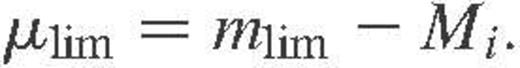 . (In other words, μlim is the maximum distance modulus at which a galaxy of absolute magnitude Mi would be observable.) The logarithm of the cumulative luminosity function F(M) can afterwards be estimated from the equation
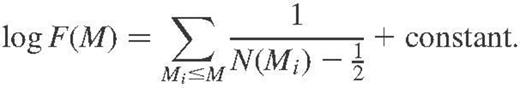
For further details, see for example Efron & Petrosian (1992).
Note that the C− method may be applied to data of arbitrary spatial distribution — i.e. no assumption concerning spatial homogeneity is required. Thus, the C− method provides an estimate of the luminosity function — or, in the present context, the diameter function — that requires no correction for Malmquist bias. In both respects, therefore, it is considerably more robust than existing techniques for calibrating H0. The method is, however, applicable only to samples that are strictly complete to a given apparent magnitude or isophotal diameter — i.e. where the selection function in angular diameter is well described by a sharp cut-off. We have also, therefore, developed an objective test of the validity of this assumption, based on the statistical technique proposed by Efron & Petrosian (1992). (See Section 4 below and Rauzy 2001 for more details.)
The only remaining assumptions to which our method is subject are as follows:
- (i)
the distribution function reconstructed from the distant sample is not significantly affected by peculiar motions;
- (ii)
the local calibrating galaxies represent an unbiased sample from the distribution function reconstructed from the distant sample.
We note that both of these assumptions are, of course, inherent in all other H0 determinations using galaxy distance indicators. Note also that the method may be used as a robust test of specific peculiar velocity field models, and to estimate the linear bias parameter β (Rauzy & Hendry 2000).
3 Application using galaxy linear diameters: systematic bias in the calibrating sample?

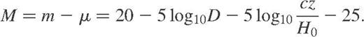
We compared the CDF of M reconstructed from the LEDA galaxies with the sample CDF of M obtained from a set of 14 local calibrating galaxies with Cepheid distances determined by HST. Table 1, based on data from Theureau et al. (1997), summarizes the data for the local calibrators. We then varied H0 in equation (3) for the reconstructed LEDA CDF and, for each value of H0, determined the Kolmogorov–Smirnoff (KS) distance Δ, defined as the maximum vertical deviation between the two CDFs as a function of M.
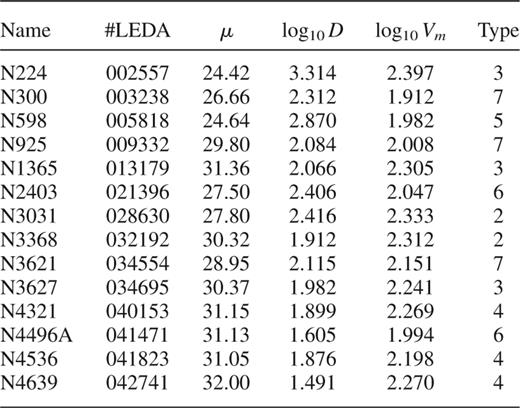
Local calibrating galaxies, from Theureau et al. (1997). Distance moduli, μ, were determined from HST observations of Cepheid variables. Following GGH97, linear diameters, D, are corrected for galactic extinction, but not for inclination.
We obtained a ‘best-fitting’ value of H0 (namely 42 km s−1 Mpc−1), which gave the minimum KS distance, Δmin. This value agreed well with those reported by Sandage (1993a,b), who used linear diameter as a ‘standard ruler’ distance indicator calibrated by M31 and M101, respectively. It was also consistent with the analysis of GGH97, who obtained H0=52±6±8 km s−1 Mpc−1 using galaxy linear diameters from the RC3 catalogue (de Vaucouleurs et al. 1991), calibrated by a sample — very similar to that used here — of 12 spirals with HST Cepheid distances.
The second uncertainty quoted by GGH97, however, was an estimate of the possible error in H0 due to a systematic difference in the mean intrinsic diameter of the local calibrating galaxies compared with the distant sample (even after correction for Malmquist bias). In particular, GGH97 suggested that the mean diameter of the local calibrators might be systematically larger than that of the distant sample, given the strategy of the HST Key Project to observe ‘Grand Design’ spirals (Kennicutt et al. 1995). This would lead to a systematic underestimation of H0 from galaxy diameters, bringing the value reported by GGH97 into closer line with most other recent estimates.
We found evidence in Hendry & Rauzy (2000) for such a systematic bias in the mean diameter of the calibrators, since it appeared that galaxies of small diameter are relatively under-represented in the CDF of the local calibrating sample. Hence our remaining assumption — that the local calibrating galaxies fairly sample the reconstructed LEDA diameter function — would seem to be questionable. Little further progress could be made using only galaxy diameter information, however, because of the large intrinsic spread of the diameter distribution function.
4 Including Tully–Fisher information
In this paper we improve our analysis by introducing the galaxy rotation velocity as a second parameter, to reduce the dispersion of the galaxy diameter distance indicator. This is, of course, analogous to the conventional Tully–Fisher relation but — crucially — retains completely the robustness of our previous analysis. We applied our analysis to the KLUN sample of spiral galaxies (cf. Theureau et al. 1997). In a similar manner to the recent application of the ‘Sosie’ method (cf. Paturel et al. 1998), we proceed by selecting, for each local calibrator, the subset of galaxies from the distant sample with similar log rotation velocity (within the range ±0.05) and morphological type (within the range ±1) as the calibrator. For each subset we then reconstruct the diameter function (again, in terms of the transformed variable, M) for the distant galaxies, assuming initially a fiducial value of H0=100 km s−1 Mpc−1.
4.1 A robust statistical test of completeness
In order to apply our reconstruction method to the subset of the KLUN sample with log rotation velocity and morphological type similar to each of the local calibrators, we require first to identify the diameter limit (or equivalently the magnitude limit, in terms of the transformed variable, m) up to which the selection function of the sample may be reasonably approximated by a Heaviside function.
Rauzy (2001) describes a robust statistical test for completeness, closely based on the method first proposed by Efron & Petrosian (1992) for analysing truncated data sets. The test is based on constructing a statistic, TC, that has expectation zero and variance unity under the null hypothesis of a complete sample (and independent of any assumption about the spatial distribution and the luminosity or diameter function of the galaxies). Beyond the limiting magnitude or limiting diameter, on the other hand, TC becomes systematically more negative. One can, therefore, estimate the completness limit for each subset of the KLUN sample by determining the value of the test statistic, TC, as a function of apparent magnitude and identifying the magnitude at which TC becomes significantly negative.
Note that, in defining the completeness limit and reconstructing the galaxy diameter or luminosity function, it is important to consider the possible effects of extinction. The ‘raw’ apparent magnitudes and (to a lesser extent) isophotal diameters of the distant sample will be affected by a Galactic extinction term that varies with direction, and — in principle — by an internal extinction term that depends on the axis ratio (i.e. the inclination) of the galaxy. Strictly, therefore, the ‘sosies’ of a given local calibrating galaxy should be selected to have similar galactic extinction and axis ratio as the calibrator, otherwise the comparison between the diameter of the calibrator and the reconstructed ‘sosie’ diameter function could lead to a biased estimate of H0. An extended ‘sosie’ definition along these lines was adopted in Paturel et al. (1997). The effect of Galactic extinction can more easily be dealt with, however, by simply using corrected apparent magnitudes and isophotal diameters in applying the completeness test and reconstruction procedure, although in so doing we will, of course, reduce slightly the number of galaxies in each ‘sosie’ sample. We adopt this approach throughout this paper. Following GGH97 and references therein, however, we do not apply an (inclination-dependent) correction for internal extinction. We discuss in Section 6 the possible bias in H0 that could arise owing to (uncorrected) internal extinction.
Fig. 1 illustrates the application of the completeness test to the sample of ‘sosies’ of the calibrator N4536. The upper panel shows a standard plot of the number of galaxies as a function of apparent magnitude — the method that has generally been used in the past to estimate the completeness limit subject to the assumption of an underlying galaxy distribution that is homogeneous. Note, however, that the predicted variation in number counts with magnitude — shown by the grey line in this case (i.e. a slope of 0.6 in log N) — is a poor fit to the real data, indicating that the assumption of homogeneity is not justified, or that selection effects in distance (i.e. redshift) are present in the sample. The lower panel, on the other hand, shows the value of the test statistic as a function of limiting apparent magnitude; also shown are lines indicating the expectation value, T¯C, and  . It can clearly be seen that the test statistic is consistent with zero (i.e. within 1 σ) for m*<13.9 and systematically negative for m*≥13.9, which corresponds (from equation (2) to a diameter limit of Dcor=1.66′. Similar results were obtained when the completeness test was applied to subsets of the KLUN data containing ‘sosies’ of the other calibrators; see Section 5 below.
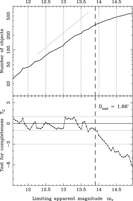
Completeness tests for the N4536 ‘sosies’ sample. Upper panel shows the number counts of galaxies brighter than a given apparent magnitude and the straight line prediction for an underlying homogeneous galaxy distribution. Lower panel shows the value of our robust completeness test statistic as a function of limiting apparent magnitude. The adopted magnitude limit of 13.9 corresponds to a diameter limit of Dcor=1.66′.
4.2 Reconstruction of the cumulative diameter function and the impact of peculiar motions
Having identified an appropriate apparent magnitude limit, the next step in our method is to reconstruct a robust estimate of the cumulative diameter function, expressed in terms of absolute magnitude. We first illustrate this step for the case of the N4536 sosies in the KLUN sample. Fig. 2 shows a histogram of the redshifts of the N4536 sosies, complete in apparent magnitude up to  . The median redshift of this sample of 322 galaxies is cz≃3250 km s−1, suggesting that the first of our two remaining assumptions — that the reconstructed distribution function is not significantly affected by peculiar motions — is reasonable.
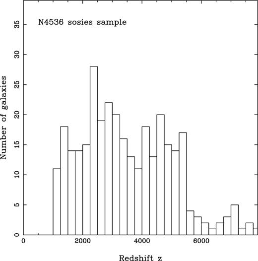
Redshift histogram for the N4536 sosies sample complete to an apparent magnitude limit of mlim=13.9. Median redshift for this sample is cz≃3250 km s−1.
Fig. 3 shows the reconstructed cumulative diameter for the N4536 sosies, after correction for peculiar velocities according to three different schemes:
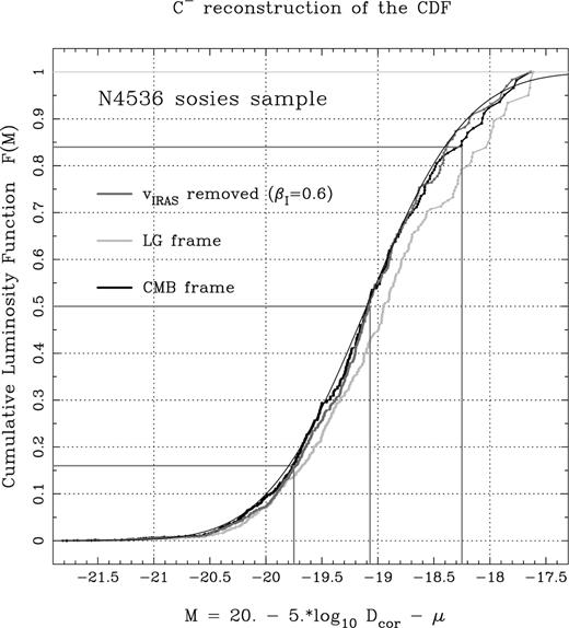
Reconstructed cumulative diameter function for the sosies of N4536 in the KLUN sample. CDFs are shown derived from redshifts first corrected to the CMBR frame (black curve) corrected for the peculiar velocities determined from the IRAS 1.2 Jy predicted velocity field with βI=0.6 (dark-grey curve) and corrected for a model of the Local Group motion (light-grey curve). Also shown are the best-fitting Gaussian curve with median value and 1-σ percentiles indicated.
- (i)
corrected to the CMBR frame, shown as the thick black curve;
- (ii)
after removal of the IRAS 1.2 Jy predicted velocity field, assuming βI=0.6 (Strauss, private communication), shown as the thick dark-grey curve;
- (iii)
corrected for the motion of the Local Group derived by Yahil, Tammann & Sandage (1977), shown as the thick light-grey curve.
Also shown is the best-fitting Gaussian CDF curve, and the median and 1-σ percentiles for the CMBR-corrected case.
We can see from this figure that the scheme adopted to correct for peculiar velocities does have a small impact on the reconstructed CDF. In particular, the results obtained using the Local Group-corrected redshifts show a clear discrepancy from those for the other two cases. Agreement between the CMBR-corrected case and the IRAS-corrected case is excellent, however. Moreover, the Local Group-corrected reconstruction differs in median value from the other two cases by only ∼0.1 mag. This is a consequence of the fact that our method makes use of distant galaxies in the KLUN sample, as was clear from Fig. 2, so that for much of the subsample the impact of different peculiar velocity models (or indeed no peculiar velocity model) is negligible. Similar results were obtained for the other sosie samples. This robustness to the peculiar velocity field marks an important difference between our method and previous similar treatments using galaxy diameters to estimate H0, since they have generally restricted their data sets to nearby samples, as we next discuss.
4.3 Comparison with ‘plateau’ methods
Both the Spanhauer method (Sandage 1994) and the method of normalized distances (Teerikorpi 1984; Bottinelli et al. 1986) are based around the principle of identifying a ‘plateau’ region of galaxies that are not significantly affected by selection bias. (Indeed both of these methods are essentially more sophisticated developments of the ‘bias-free subset’ concept introduced by Sandage & Tammann 1975– see Teerikorpi 1997 for a very clear discussion of the relationship between these different methods.) The drawback with the plateau approach, therefore, is that one is discarding more distant data in favour of nearby galaxies that — although not significantly affected by selection bias — will be more seriously contaminated by peculiar motions.
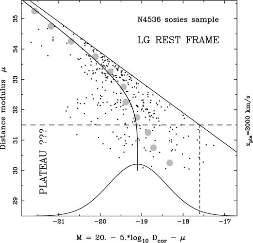
As an illustration of the impact of peculiar motions on plateau methods, Fig. 4 shows a plot of (kinematic) distance modulus, μ, as defined in equation (3) with H0=100 km s−1 Mpc−1, versus absolute magnitude, for the N4536 sosies sample. The diagonal line denotes the adopted apparent magnitude limit, mlim = 13.9. Also shown at the bottom of the diagram is a schematic of the best-fitting Gaussian luminosity function fitted to the data using the C− method, as in Fig. 3 above. The solid curve shows the predicted mean absolute magnitude as a function of distance modulus for observable galaxies, assuming this luminosity function, while the grey circles indicate the sample mean absolute magnitude in distance modulus bins of width Δμ=0.5. We can see from the solid curve that one can indeed define a plateau, at cz≃2000 km s−1 below which the absolute magnitudes are not significantly affected by selection bias. Note, however, that the sample mean absolute magnitudes of galaxies in this redshift range are in relatively poor agreement with the predicted values — a discrepancy due in part to the small number of galaxies and in part to the likely impact of peculiar velocities. On the other hand, for more distant galaxies — which would be excluded in the plateau methods — the agreement between the predicted and sample mean absolute magnitude is much better.
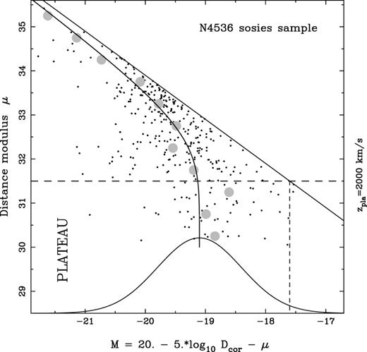
Illustration of the impact of peculiar velocities for nearby galaxies identified in plateau-based methods. For the N4536 sosies sample the solid curve shows the predicted mean absolute magnitude as a function of (kinematic) distance modulus assuming a Gaussian luminosity function and a sharp apparent magnitude limit. The grey circles indicate the sample mean absolute magnitude in a series of distance modulus bins. Note the relatively poor agreement between the predicted and sample mean values within the plateau region of the diagram.
An alternative approach to the problem of peculiar motions and their impact on estimates of H0 is to restrict attention only to nearby galaxies and correct their observed redshifts according to a detailed parametric model of the velocity field in the Local Supercluster. Willick & Batra (2001) adopt this approach and derive H0=92±5 km s−1 Mpc−1. This method is still vulnerable, however, to systematic errors in the modelled peculiar velocity field: in other words, applying the wrong peculiar velocity correction to nearby galaxies may be worse than applying no correction at all. Fig. 5 illustrates this point, showing a similar plot to Fig. 4 but now with the distance moduli computed after first correcting for the Local Group motion of Yahil et al. (1977). Note that, in this case, the sample mean absolute magnitude values within the putative plateau region are in even poorer agreement with the predicted mean values, although again the agreement is very good for more distant galaxies. More specifically, the sample and predicted mean values differ by more than 0.5 mag — i.e. a discrepancy at least five times larger than the difference in median values shown in Fig. 3 for different velocity field models. Thus, the inclusion of more distant data in the application of our robust method substantially reduces the impact of peculiar motions on our results.
As for Fig. 4 but now with distance moduli computed after first correcting observed redshifts by the Local Group model of Yahil et al. (1977). Note that the agreement of the predicted and sample mean absolute magnitudes within the (putative) plateau region is now even more questionable.
5 Results: the value of H0
The completeness test described in Section 4.1 was applied to the KLUN sosies samples of all 14 local calibrators. Note that two pairs of calibrators possess common sosie samples: N4321 and N4639, and N4496A and N925. The value of the test statistic TC is shown as a function of adopted apparent magnitude limit and is shown in Fig. 6 for each of the 12 sosie samples. A common completeness limit of mlim=13.9 was adopted.
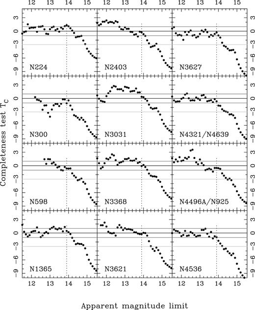
Completeness test for the 12 sosies samples of the 14 local calibrators. A common completeness limit of mlim=13.9 was adopted for all the samples.
Using this apparent magnitude limit, we carried out C− reconstructions of the cumulative diameter function for each sosie sample. We derived absolute magnitudes using CMBR-corrected redshifts. Our results are shown in Fig. 7; in each panel the best-fitting Gaussian distribution, together with the median value and the 1-σ percentiles, are indicated. The CDFs for the sosies of N300 and N598 are shown in grey; for these two samples the evidence is less clear that the CDF has ‘turned over’, so that the sample median is a robust estimate of the true median for galaxies of this sosie class. It is interesting to note that N300 and N598 have the smallest rotation velocities of the 14 calibrators, which suggests — via the Tully–Fisher relation — that they (and hence also their sosies) are among the intrinsically faintest and smallest in the calibrating sample. In other words, the effect of the magnitude cut-off may mean that the selected sosie subsamples for these two galaxies do not completely recover the faint-end tail of the distribution function.
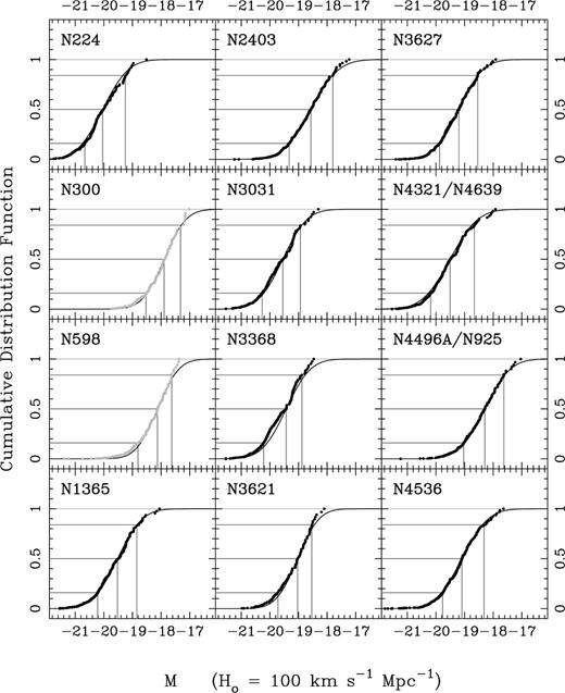
Reconstructed CDFs for the sosie distributions of the 14 local calibrators. Also shown are the best-fitting Gaussian CDF curves, with horizontal lines on each panel indicating the median and 1-σ percentiles.
The final step of our analysis is to determine individual estimates of H0 for each calibrator by determining the value of H0 required to match the median of the reconstructed sosie CDF to the absolute magnitude inferred for that calibrator from its published HST Cepheid distance. Fig. 8 shows a plot of the estimated value of the (natural) logarithm of H0, with the associated 1-σ error computed from the 68 per cent percentiles of the reconstructed CDF, for each calibrator. The estimates for N300 and N598 are shown in grey.
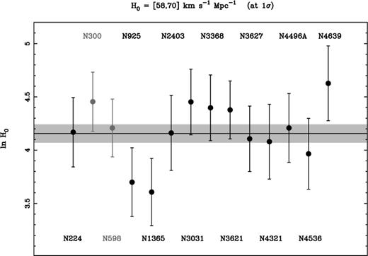
Estimates of (the natural logarithm of) H0 obtained for each of the 14 local calibrators. Errors were determined from the 68 per cent percentile of the reconstructed CDF of the sosies of each calibrator.
Thus, although we choose to adopt the latter value as our estimate of H0, the exclusion of N300 and N598 would clearly have negligible impact on our results.
6 Discussion
When we incorporate information on the rotation velocities of the local calibrators in reconstructing the KLUN diameter functions, our results are in good agreement with recent determinations of H0 from the conventional Tully–Fisher relation (cf. Giovanelli et al. 1997; Sakai et al. 2000) and the HST KP ‘final’ value (Mould et al. 2000). However, our analysis is completely free of assumptions about the form of the galaxy diameter and luminosity function and the conditional distribution function of diameter at a given value of log Vm. We do not, for example, require to assume that this conditional distribution is Gaussian, nor indeed even that it has zero mean or constant dispersion — as is often assumed in calibrating the Tully–Fisher relation. In particular, therefore, we do not require that the Tully–Fisher relation is a straight line, nor that the distribution of residuals is symmetrical. Our method would remain applicable if, for example, the distribution of Tully–Fisher residuals displayed a long ‘tail’ for galaxies of small rotation velocity (which we may see some tentative evidence for in the reconstructed CDFs of the sosies of N300 and N598). Our method is also completely independent of Malmquist bias corrections, so that our results are unaffected by the precise ‘recipe’ adopted to correct for Malmquist bias.
As we remarked in Section 4.1, we have not applied a correction for internal extinction to the local calibrators or distant galaxies. Following GGH97, we have preferred to adopt the conclusion of the authors of RC3 (de Vaucouleurs et al. 1991), who found the galaxy discs to be ‘substantially optically thick’ at the relevant isophotal level. In this case there would be no inclination dependence on the column depth of luminous material visible at a given point on the disc, so that no inclination correction to the diameter is required. It can be argued, on the other hand, that there is a substantial dependence of optical depth on inclination, so that a failure to correct for internal extinction might lead to a correlation between the axis ratio of the local calibrating galaxies and the estimated value of H0. Fig. 9 shows a scatterplot of the logarithm of the axis ratio at R25 versus the natural logarithm of H0 for each calibrator. It is clear from this figure that no significant correlation between axis ratio and H0 was present, suggesting that the impact of any uncorrected internal extinction on our final estimate of H0 would be negligible.
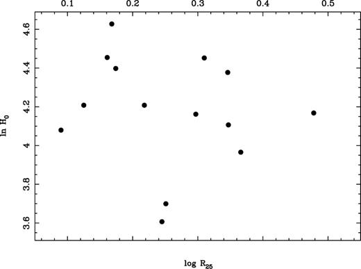
Scatterplot of the logarithmic axis ratio at isophote R25 versus the natural logarithm of H0 obtained for each of the 14 local calibrators. No significant correlation is found.
In summary, the robustness and assumption-free nature of this method has important ramifications for any current debate on the cosmic distance scale. There appears to be little possibility of any remaining systematic error in H0 that is introduced at the stage of linking the primary and secondary distance scales. Improving the calibration of the Cepheid distance scale, via the lowest rungs of the Cosmic Distance Ladder, must now be the main priority for the Distance Scale community.
Acknowledgments
We are thankful to Michael Strauss for providing us with the predicted IRAS peculiar velocity model, and to the anonymous referee for helpful comments. SR acknowledges the support of the PPARC, and SR and MAH acknowledge the use of the Starlink computer node at the University of Glasgow.
References
