A comparison of the anelastic and subseismic approximations for low-frequency gravity modes in stars

Abstract

1 Introduction

Initiated with the work on atmospheric convection by Ogura & Phillips (1962) and Gough (1969), the anelastic approximation has been widely used in astrophysics to describe compressible convection. For example, it has been first applied by Latour et al. (1976) and Toomre et al. (1976) to investigate the non-rotating and non-magnetized convective envelopes. Then, Gilman & Glatzmaier (1981) and Glatzmaier & Gilman (1981a–c) extended these studies to the rotating case, whereas the magnetohydrodynamic (MHD) case has been considered by Glatzmaier (1984, 1985a,b), Lantz & Sudan (1995) and Lantz & Fan (1999).

In all of these studies, this approximation has been preferred to an other famous one in fluid dynamics, the so-called Boussinesq approximation where the velocity is assumed to be solenoidal, i.e. (Spiegel & Veronis 1960). As the density varies over several orders of magnitude in a convection zone, using the anelastic approximation is indeed more relevant and leads to . However, both approximations filter out short-period acoustic oscillations by assuming that the Mach number of the convection is small so that ‘the task of numerical solution will not be complicated by the need to resolve very rapid time variations’ (Latour et al. 1976).

More recently, the anelastic approximation has been used in the field of stellar oscillations. Waves can propagate over long distances in star interiors and large variations of density also need to be taken into account. Thus, as in stellar convection studies, the Boussinesq approximation is too restrictive and not adapted for this problem. However, since acoustic waves are filtered out, only the low-frequency part of the oscillations spectrum is captured. As this part of the spectrum also corresponds to the most perturbed one when rotation acts, this approximation is very attractive when low-frequency modes of a rotating star are considered.

Understanding the spectrum of rotating stars is indeed a difficult problem when the rotation period is of the same order as the oscillation one. In this case, the usual perturbative theory of Ledoux (1951) reaches its limits and the eigenvalue problem needs to be solved non-perturbatively (Dintrans & Rieutord 2000; hereafter referred to as Paper I). However, rotation introduces new computational challenges:

• (i)

  the strong Coriolis coupling between normal modes of different degrees (ℓ, ℓ± 1) leads to a large system of coupled differential equations;

• (ii)

  some singularities owing to the presence of wave attractors emerge in the region σ ≃ 2Ω, where σ is the wave frequency and Ω is the uniform rotation rate of the star.

Applying the anelastic approximation does not remove these singularities but decreases the size of the numerical problem since acoustic quantities disappear (see Paper I). We note that Berthomieu et al. (1978) used the same arguments when considering a hierarchy between the displacement and pressure components, this hierarchy leading to the same result as the direct use of the anelastic approximation.

In contrast to stars, the mass of the Earth is not strongly concentrated near its centre. Only 30 per cent of the whole mass is indeed inside the half radius, whereas this ratio is around 90 per cent for the Sun (see, e.g., Stix 1989). It means that the variations in density in the Earth's outer fluid core generated by the propagation of seismic P-waves may produce non-negligible variations in the gravitational potential φ and explains why geophysicists do not wish to use the Cowling approximation in their description of P-waves. To take into account this effect but to simplify the equations for low-frequency modes Smylie & Rochester (1981) and Smylie, Szeto & Rochester (1984) introduced the ‘subseismic’ approximation where self-gravity is included.

Recently, De Boek, Van Hoolst & Smeyers (1992) applied this approximation to describe the low-frequency g-modes of non-rotating stars. Starting from the same equations as Smylie & Rochester (1981), they found an analytic expression for the asymptotic low frequencies that slightly differs from the standard one deduced by Tassoul (1980) in the Cowling approximation. By applying this expression to the low-frequency oscillations of both homogeneous and polytropic (n = 3) star models, De Boek et al. (1992) concluded that the subseismic approximation is more accurate than the standard one in the polytropic case but less accurate in the homogeneous case.

However, as will be shown below, the subseismic approximation is not a consistent approximation of the equations of motion; indeed, we will show that the proper way to simplify the equations in order to deal with the low-frequency modes is to use the anelastic approximation and that this approximation also implies Cowling's approximation.

Hence, after establishing the complete set of equations describing linear oscillations of a stratified compressible fluid and the appropriate boundary conditions (Section 2), we focus on the similarities and differences of the anelastic and subseismic approximations (Section 3); in particular, we show that both imply Cowling's approximation and demonstrate the inconsistency of the subseismic approximation. Then we compare the two approximations on the test cases used by De Boek et al. (1992), namely, the homogeneous and polytropic star models (Section 4). Comparison of the resulting approximate eigenfrequencies with the exact ones (computed numerically for the polytrope but analytically for the homogeneous model) shows clearly the better efficiency of the anelastic approximation. Finally, we conclude in Section 5 with some outlooks of our results.

2 The basic equations

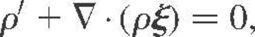
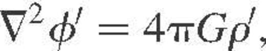
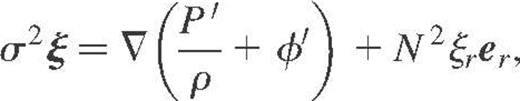
Assuming a time dependence of the form exp(iσt), the governing equations that describe the adiabatic oscillations of a spherically non-rotating star are given by

(1)

(2)

(3)

(4)

where P′, ρ′ and φ′, respectively, denote the Eulerian fluctuations of pressure, density and gravitational potential, whereas δP, δρ and ξ are the Lagrangian fluctuations of pressure, density and displacement such as

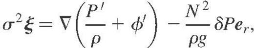
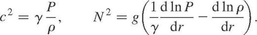
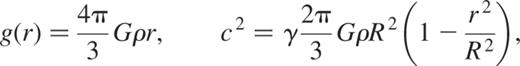
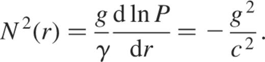
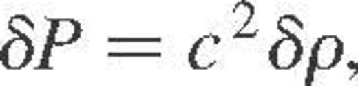
with a pressure gradient satisfying the hydrostatic equilibrium . Also, ρ is the equilibrium density, g the gravity and the first adiabatic exponent. Finally, c² and N², respectively, denote the squares of the velocity of sound and Brunt–Väisälä frequency such as

(5)

In order to obtain a well-posed eigenvalue problem with an eigenvalue σ², boundary conditions should be stipulated at the star centre and surface. At the centre, we impose the regularity of all pulsation quantities such as (see, e.g., Unno et al. 1989)

(6)

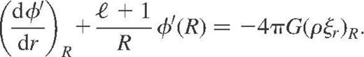
where ℓ denotes the spherical harmonics degree of the eigenmode. At the surface, which is assumed to be free, we impose the following condition coupling ξ_r and φ′ (Ledoux & Walraven 1958)

(7)

Finally, we adopt the classical mechanical outer condition for the pressure which reads

(8)

3 The subseismic and anelastic approximations applied to stellar oscillations

3.1 The common properties

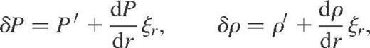
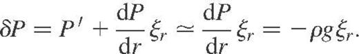
Since the work of Cowling (1941), it has been well known that g-modes are mainly transverse, whereas p-modes are predominantly radial. The Eulerian pressure and density perturbations are thus small for a g-mode and both subseismic and anelastic approximations take advantage of that by assuming that the Lagrangian pressure fluctuation δP is only caused by the radial displacement one; i.e. the Eulerian fluctuation P′ does not contribute and we have

(9)

In this case, equations (2)–(4) now read as

(10)

(11)

(12)

At this stage, two important consequences appear.

• (i)
  As observed by De Boek et al. (1992), the radial Lagrangian displacement necessarily vanishes at the surface. To show this, we take the radial component of equation (10)

  
  The problem arises from the fact that the Brunt–Väisälä frequency diverges as 1/c² at the star surface (see equation 5). Thus, as N² diverges to infinity at , ξ_r must vanish at this point to avoid a singular radial displacement. In the complete case (i.e. when acoustic waves are included), we note that it is the mechanical condition which permits a finite radial displacement at the surface, as shown by the radial component of equation (2)

  

  where the term N²/(ρg) diverges as 1/(ρc²). Thus, the subseismic and anelastic ξ_r-eigenfunctions always have one node less than their corresponding unapproximated eigenfunctions for which ξ_r(R) is finite.
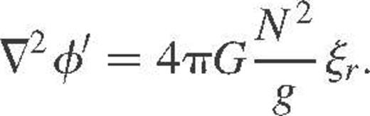
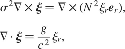
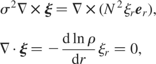
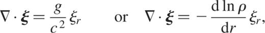
• (ii)
  The second consequence, which is not straightforward, is that the use of the subseismic or anelastic approximation necessarily implies Cowling's approximation where the perturbations φ′ are neglected (Cowling 1941). To show this, we first take the curl of equation (10) and obtain

  

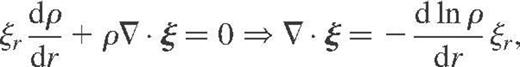
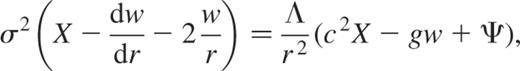
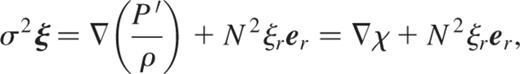
  Furthermore, combining equations (1) and (11) allows us to find the following subseismic form for the equation of mass conservation,

  

  (13)

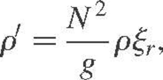
  whereas, as shown in the introduction, the anelastic counterpart of this equation reads

  

  (14)
  The two different forms (13) and (14) may be formally written as , where ℒ denotes a differential operator depending on the approximation we use. We thus have to deal with the following new system:

  

  (15)

  

  (16)

  

  (17)

  whereas the surface boundary conditions now read

  

  It is thus clear that the Poisson equation (17) decouples from equations (15) and (16). In other words, the knowledge of equations (15) and (16) with the boundary condition is sufficient to find the set of eigenfrequencies σ². The gravitational potential perturbation φ′ does not act on the determination of σ² and can be seen as ‘slaved’ to ξ_r via equation (17).¹ We note that Smylie & Rochester (1981) do not clearly emphasize this point and just noticed that the φ′-perturbations can be determined after solving their subseismic equations for velocity and reduced pressure.

3.2 The main difference

As shown above, the subseismic and anelastic approximations do not lead to the same equation of mass conservation since the term stemming from the density perturbations is kept in the subseismic case (see equations 13 and 14). We will now show that the subseismic form of this equation is in fact not correct because it is not consistent with the basic assumption from equation (9).

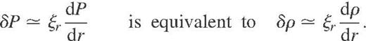
First of all, we recall that both approximations assume that the Eulerian pressure perturbation does not contribute to the Lagrangian one, that is

(18)

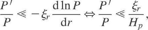
where denotes the pressure scaleheight. Moreover, we can relate the Eulerian pressure and density perturbations using equation (3) as

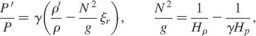
where denotes the density scaleheight and where equation (5) has also been used. Therefore, the basic assumption from equation (18) leads to

(19)

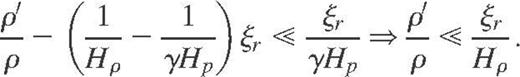
This last equation is important since it shows that we can also neglect the Eulerian contribution ρ′ in the Lagrangian perturbation δρ when equation (9) is assumed, i.e. we have

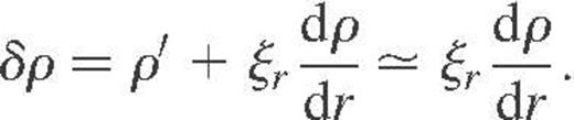
In other words, if we just take into account the contribution stemming from the equilibrium pressure gradient in δP, we should also do the same with the contribution coming from the equilibrium density gradient in δρ. Hence

(20)

We can now easily understand why the subseismic equation of mass conservation is not correct. Equation (1) indeed gives

In order to be consistent with the basic assumption from equation (20), the equation of mass conservation now reads

and we recover the good anelastic form (14).

The subseismic form of mass conservation (13) of Smylie & Rochester (1981) is therefore clearly inconsistent because of its incompatibility with the hypothesis (9). Consequently, the subseismic approximation is necessarily less accurate than the anelastic one as we will now show.

4 Results

In order to test the efficiency of both approximations, we applied the following procedure to the oscillations of the homogeneous compressible star (i.e. a polytrope of the order of 0) and the polytrope n = 3.

• (i)

  We first calculated the exact eigenfrequencies of the full case, that is we solved the set of equations (1)–(4) using boundary conditions (6)–(8). This has been achieved analytically for the polytrope n = 0 (Pekeris 1938) and numerically for the polytrope n = 3.

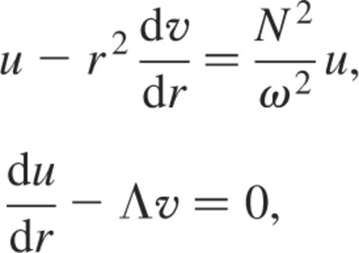
• (ii)

  Next we calculated the subseismic and anelastic eigenfrequencies by solving the system consisting of equation (15), the equation of mass conservation (13) or (14) and finally the boundary condition discussed in Section 3.1. Once again, analytical expressions have been used in the homogeneous case, whereas the polytrope has been computed numerically. The efficiency of both approximations has been deduced by a direct comparison between these approximated eigenfrequencies and the previous exact ones.

4.1 The homogeneous polytrope

As a first example, we concentrate on the unstable second-degree g⁻-modes of the polytrope inline-graphic n = 0. Pekeris (1938) first studied the non-radial oscillations of this model and found the exact g⁻-eigenfrequencies as

where and

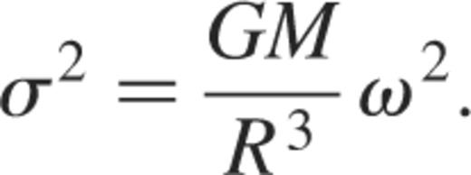
Here ω² denotes the dimensionless eigenfrequencies, which for a star of mass M and radius R, are related to the σ² ones by

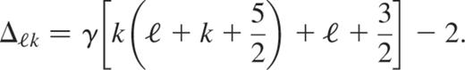
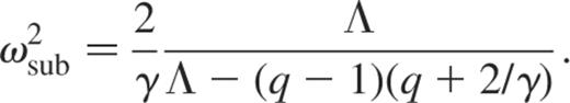
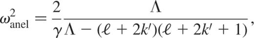
Using an equivalent method to that used by Pekeris (i.e. the search of a power-series solution), we calculated the analytic expressions of the subseismic and anelastic eigenfrequencies of the homogeneous polytrope and found (see appendix A)

(21)

(22)

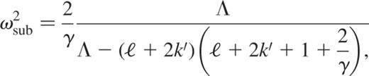
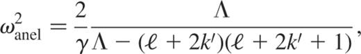
where .

We summarize in Table 1 the exact eigenfrequencies calculated for the homogeneous star with , and various orders k, whereas Fig. 1 gives the relative errors (in per cent) made with both approximations for the first 30 g⁻-modes. The anelastic approximation clearly appears to be more precise than the subseismic one since, for example, the anelastic eigenfrequency at is about 20 times more precise than the subseismic one.

Table 1.

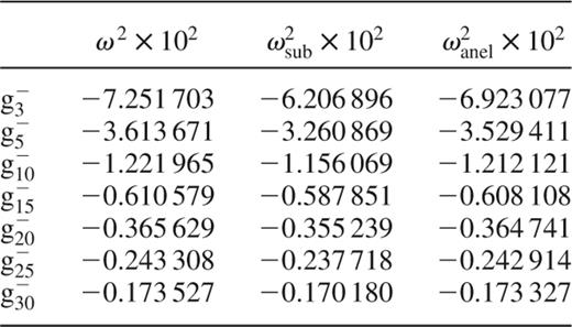
Squares of exact ω², subseismic ω²_sub and anelastic ω²_anel eigenfrequencies of the homogeneous polytrope.

Open in new tabDownload slide

Figure 1.

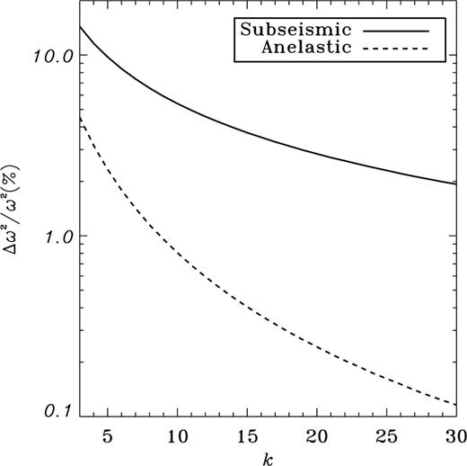
Rates of relative errors of the subseismic (equation 21) and anelastic (equation 22) eigenfrequencies as the order k increases for the homogeneous star model.

Open in new tabDownload slide

4.2 The polytrope n = 3

4.2.1 Numerics

We next calculated the second-degree g⁺-mode of the polytrope . As already mentioned, analytic expressions of eigenfrequencies are not known for this model so we computed numerically the eigenfrequencies of g⁺-modes with the complete set of equations and their approximated subseismic and anelastic counterparts. As in our preceding work (Dintrans, Rieutord & Valdettaro 1999; Paper I), we used an iterative eigenvalue solver based on the incomplete Arnoldi–Chebyshev algorithm. This numerical method differs from the classical ones where eigenfrequencies are determined by a direct integration of the governing equations using either relaxation methods (Osaki 1975) or shooting methods (Hansen & Kawaler 1994). Our eigenvalue formulation is presented in appendix B, with a discussion on the tricky problem of the degeneracy of the eigenvalue equations at the star surface when the subseismic or anelastic approximation are used.

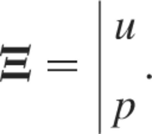
Eigenfrequencies λ² are solutions of a generalized eigenvalue problem

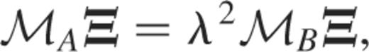
where ℳ_A, ℳ_B denote two differential operators discretized on a Gauss–Lobatto grid associated with Chebyshev polynomials and Ξ is the eigenvector associated with λ². We also note that the regular singularities appearing in the subseismic or anelastic equations at the surface are replaced by the boundary conditions (see appendix B.2).

4.2.2 Results

We summarize in Table 2 the computed eigenfrequencies (in units of 4πGρ_c) for the polytrope with , and various radial orders.² As in the homogeneous case, the anelastic approximation appears to be superior to the subseismic one. This is illustrated by Fig. 2 where we show that the anelastic relative errors are always smaller than the subseismic ones. Still for , the agreement with the true eigenvalue is of about five times better with the anelastic approximation than with the subseismic one.

Table 2.

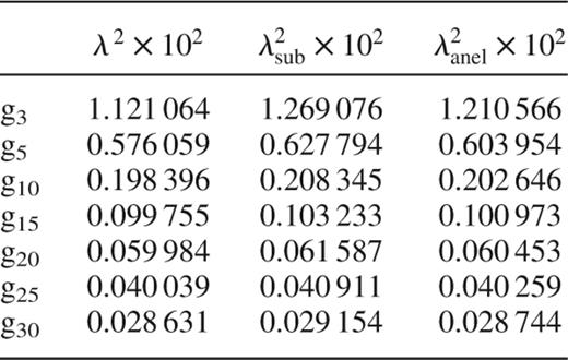
Squares of the true λ², subseismic λ²_sub and anelastic λ²_anel eigenfrequencies of the polytrope n = 3.

Open in new tabDownload slide

Figure 2.

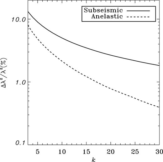
Rates of relative errors of computed eigenfrequencies for the polytrope .

Open in new tabDownload slide

We note, however, that this accuracy difference tends to be less pronounced than for the homogeneous model. In fact, the comparison of Figs 1 and 2 shows that the subseismic relative errors are the same in both cases, whereas the anelastic ones increase in the polytropic case. Therefore, dealing with a model with important density variations attenuates the differences between the two approximations.

5 Conclusion

We studied the properties of the subseismic and anelastic approximations devised for low-frequency g-modes of stars. These approximations both assume that the Eulerian perturbations of pressure do not contribute to their Lagrangian parts. Consequently, acoustic waves are filtered out. However, the equation of mass conservation differs since the subseismic approximation keeps the contribution coming from the Eulerian density fluctuation. We showed that this is incorrect because it is inconsistent with the neglect of the Eulerian pressure perturbation.

As an illustration we first applied both approximations to the low-frequency g⁻-modes of the homogeneous star. In this case, we found an analytic expression for the subseismic and anelastic eigenfrequencies using power-series solutions. We thus showed that the anelastic approximation is more precise than the subseismic one as expected.

As a second test, we considered the low-frequency g⁺-modes of the polytrope . No analytic solutions can be found for this model and eigenfrequencies have been computed numerically using an iterative solver. We thus computed the subseismic and anelastic eigenfrequencies and compared them to the exact ones. As in the homogeneous case, the anelastic approximation is more accurate than the subseismic one.

We also showed that Cowling's approximation is a necessary consequence of the anelastic approximation; it is therefore unnecessary to enforce this approximation since perturbations of self-gravity will automically decouple from the set of equations and will not influence the eigenfrequencies.

As already mentioned in the Introduction, an obvious application of the anelastic approximation concerns the low-frequency oscillations of rapidly rotating stars. Applying this approximation indeed removes the acoustic quantities and dramatically decreases the size of the numerical problem. An example is given in Paper I with the study of the oscillations of a rapidly rotating γ Doradus-type star, for which periods of oscillations are of the same order as that of rotation (i.e. around 1 d).

Acknowledgments

BD has been supported by an ATER position at Université Paul Sabatier and now by the European Commission under Marie-Curie grant no. HPMF-CT-1999-00411 which are gratefully acknowledged.

References

Appendix

Appendix A:Analytic expressions for the homogeneous star model

A.1 The subseismic case

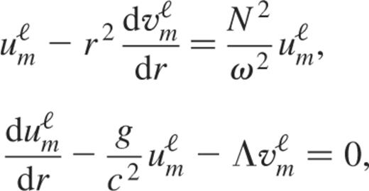
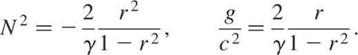
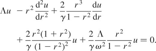
We start from equations (15) and (13)

(A1)

where g, c² and N² are given by

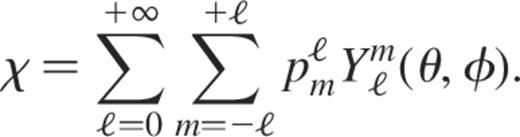
The star radius is the length-scale and the dynamical time is the time-scale. In addition, we expand the spheroidal eigenvectors ξ on spherical harmonics as (Rieutord 1987)

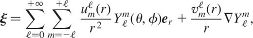
where denotes the normalized spherical harmonics. We thus obtain the same radial equations coupling and as De Boeck, Van Hoolst & Smeyers (1992), namely

(A2)

where and

Eliminating leads to the equation for alone (for clarity, we drop the subscripts ℓ and m)

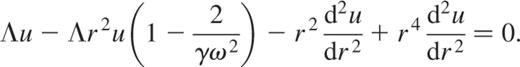
After some algebra, this last equation may be written

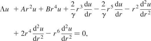
where

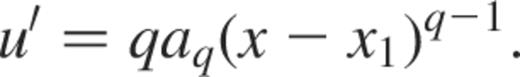
We now expand u(r) in a power-series of r such as

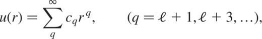
where we took into account that near the centre. We thus obtain the following difference equation for the c_q coefficients

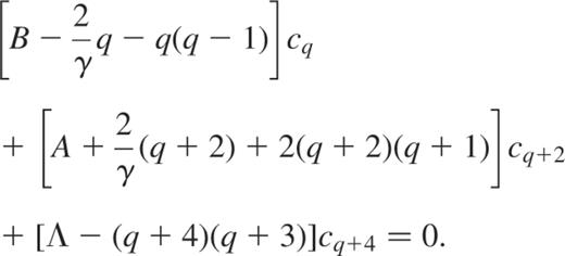
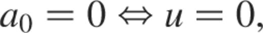
The convergence of the series implies that

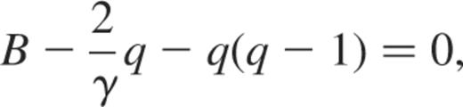
which leads to the following expression of the subseismic eigenfrequencies:

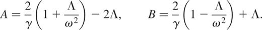
In order to have an easy connection with the eigenfrequencies of the unapproximated case, we adopt and finally obtain

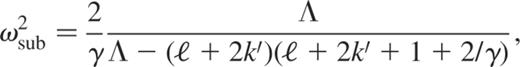
with .

A.2 The anelastic case

We start now from equations (15) and (14)

(A3)

where we used the fact that ρ is a constant for the homogeneous star. Thus, by applying the same formalism as above, we obtain the following anelastic radial equations for u and v

(A4)

and the equation for u alone now reads

As in the subseismic case, we look for a power-series solution which leads to the following difference equation:

The convergence of the series requires that

and we deduce the anelastic eigenfrequencies of the homogeneous star as

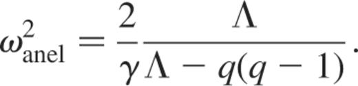
As before, we adopt and obtain

with .

Appendix B: The eigenvalue problem for the polytrope n = 3

In this appendix, we formulate the oscillation equations as a generalized eigenvalue problem and discuss the ‘degeneracy’ of these equations at the star surface when the subseismic or anelastic approximation is applied.

1.B The complete case

The governing equations we need to solve are equations (1)–(4) with boundary conditions (6)–(8). The aim is to derive a generalized eigenvalue problem of the form

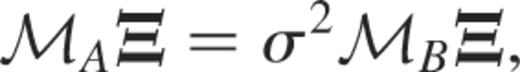
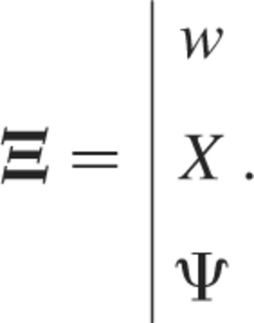
where ℳ_A and ℳ_B denote two differential operators. Here Ξ is the eigenvector associated with the eigenvalue σ²; it may read, for instance,

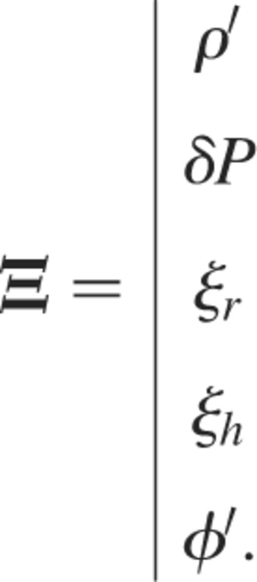
These equations are clearly not well adapted for an eigenvalue problem formulation since equations (1), (3) and (4) lead to three lines of zeros in the matrix ℳ_B making the system not well-conditioned for iterative solvers.

We therefore prefer to use the oscillation equations of Pekeris (1938) who obtained, after judicious substitutions, the following reduced system (its equations 12, 14 and 15; see also Hurley, Roberts & Wright 1966)

(B1)

(B2)

(B3)

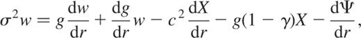
where (should not be confused with the dimensionless eigenfrequencies ω), and , ψ being the gravitational potential perturbation.

In order to obtain the simplest dimensionless polytropic equations, we choose two new length- and time-scales. As length-scale, we take R/x₁, whereas is our time-scale. Here x₁ is related to P_c and ρ_c by (see, e.g., Hansen & Kawaler 1994)

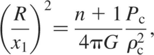
where P_c and ρ_c, respectively, denote the central pressure and density of the polytrope. With these scales, we have for example the following relations:

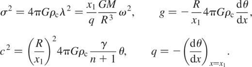
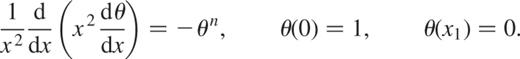
We note that for the polytrope , and . Moreover, we recall that the function θ(x) is solution of the Lane–Emden equation

(B4)

We thus obtain the dimensionless system (the prime denotes the derivative d/dx)

(B5)

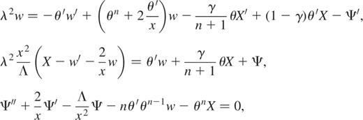
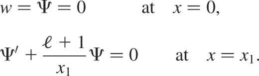
with the following set of boundary conditions:

(B6)

Systems (B5) and (B6) may still be formally written as

(B7)

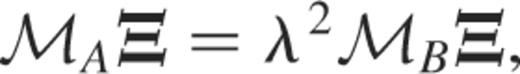
where ℳ_A and ℳ_B denote two differential operators and λ² are the real eigenvalues associated with the eigenvectors Ξ such as

B.2 The subseismic and anelastic cases

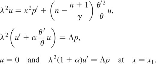
We have shown in Section 3.1 that the Cowling approximation is necessary when the subseismic or anelastic approximation are used; thus we now have to deal with

(B8)

(B9)

where we defined . By using the same scales as above and eliminating v with equation (B9), we obtain the following dimensionless system for u and p:

(B10)

(B11)

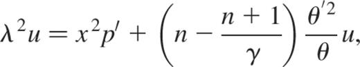
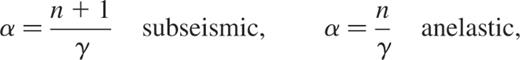
Here the parameter α differs according to the approximation used, namely

whereas is related to the projection of χ on the spherical harmonics as

At the surface, we have thus regular singularities appear in equations (B10) and (B11). To remove them, a solution would consist in multiplying these two equations by θ to obtain the new system

(B12)

(B13)

The singularities indeed disappear but are now replaced by a surface degeneracy since each equation gives the same solution at (which is, however, physically correct when using the subseismic or anelastic approximation; see Section 3.1). This is, however, making the discretized eigenvalue problem singular and this should be avoided.

Following Hurley et al. (1966), we preferred to use the Frobenius method. We first develop θ(x) near as

and, as ,

(B14)

We next expand u(x) and p(x) in series of the form

and obtain, using Einstein's notations,

Thus equation (B11) now reads

Equating the lowest power of , which is here , gives again

whereas the next power of gives

We therefore obtain the second boundary condition and the system we need to solve is

(B15)

which can be rewritten as (B7) with

This paper has been typeset from a tex/latex file prepared by the author.