Fresnel Free Imaging Mode (FFIM) for Transmission Electron Microscopy: A Computationally Mediated Solution using Spatio-Temporal Functionalization of the Illumination Optics Free

Today’s high performance Transmission Electron Microscopes (TEM), especially those equipped with aberration correctors, operate routinely at incident beam accelerating voltages between 30 – 300 kV, employ field emission sources and operate at extremely high-performance levels [1]. Importantly these advanced field emission electron beam lines have both high brightness and highly coherent beams. Due to the location of the illumination / probe forming apertures and their focal planes, Fresnel diffraction effects in the illumination system are virtually always present. This diffraction manifests itself as a series of concentric rings in the illumination of the specimen as illustrated experimentally and theoretically in Fig. 1. In this figure the experimental images were taken using the Analytical PicoProbe instrument (the prototype of the ThermoFisher Spectra UltraX) [2], while the theoretical images were calculated in Python using Fresnel diffraction theory [3, 4]. The systematic variation in spacing and contrast of the fringes at the beam center decreases with larger probes (1a, c) vs the opposite trends for the smaller probes (1b, 1d). The magnitude of which is a function of lens excitation (C1 lens/spot size), condenser aperture size and lens focus. While these interference fringes affect the local illumination intensity by introducing a periodic intensity variation at various radial distances, they do not significantly affect the post specimen scattering/optics, save for introducing an unwanted oscillation in the overall image intensity. Fresnel diffraction is mainly prominent in CTEM vs. STEM experiments in contrast to the latter, which operates closer to Fraunhofer diffraction conditions.

In the past the traditional solution to mitigate/minimize this Fresnel oscillatory illumination, which is superimposed upon the scattered image intensity, is to spread the beam and/or decrease the coherence of the illumination/probe. While this will mitigate the oscillations in the center of the illumination, as illustrated experimentally in Figs 1a and1c, it generally remains at the periphery. The second aspect of spreading the electron beam is a decrease in the overall dose illuminating an area at fixed beam current. To keep the intensity high during imaging, an analyst will frequently increase the beam current and/or exposure time to compensate for the larger area of irradiation resulting from the use of a larger electron probe. For stable non-beam sensitive materials this may not be problematic, however in today’s research environment, particularly in the situation of hard/soft materials or in single particle analysis using cryoEM of biological materials this may not be desirable as it can introduce damage artifacts due to higher dose rates [5].

An alternate solution has been developed which minimizes the Fresnel fringe [6, 7]. This is accomplished by altering the electron optical configuration, bringing into conjunction the condenser aperture instead of the condenser lens plane with the specimen plane. While this is an excellent solution, it entails realignment of the instrument, changes of various focal planes, magnification recalibration, stage/goniometer repositioning as well as numerous other adjustments, it also permits very short exposure times as is under constant low dose illumination as is sometimes required in cryoEM. For a dedicated system, which are encountered in some instruments, such as cryoEM facilities, this is a working solution, however, it is not particularly desirable in physical science multi-user systems where multiple operating modes are employed changed frequently and can be detrimental to functionality in some operating modes. This was the driving factor to devise a third alternative which is now embodied in FFIM.

The solution which was developed, requires no hardware changes or recalibration of the instrument, it is instrument agnostic and is suitable for a large range of experimental configurations. It can be turned ON and OFF, within seconds without noticeable effects on the local scattered image intensities, save for the mitigation of the oscillatory Fresnel fringe intensity superimposed upon the scattered intensity.

An example of FFIM in operation is illustrated in Figure 2, which presents a TEM image of an amorphous carbon support film with nanoscale gold islands in selected area mode (∼290 kX, I_o ∼ 100 pA, 100 um C₂ aperture, no Objective Aperture, CMOS camera). In Fig. 2a, FFIM is not enabled and the Fresnel fringes are broadly spread over the entire field of view. Fig 2b is the identical area taken only seconds later with the FFIM mode operational. Figures 3a and 3b replicate the conditions but at higher magnifications and higher resolution mode (> 550kx I_o ∼ 100 pA, 100 um C₂ aperture, no Objective Aperture, CMOS camera) showing identical effects. The beam current and exposure in all cases is nominally identical, however in the later the condenser lenses were bought closer to focus to preserve the intensity on the camera, thus changing the Fresnel fringe intensities and spacing as can be seen in Figs. 2a and 3a.

The implementation of FFIM mode is realized by dynamically changing the spatio-temporal conditions of the illumination system in real time. As can be seen by inspection of the line scans of Fig. 1e, a change in the illumination conditions will change both the probe diameter, but importantly also the position of the maxima and minima of the Fresnel fringes. This can be observed in real time by adjusting the condenser lens focus during which time the Fresnel fringes will expand and contract with the change in lens setting. Operationally FFIM is accomplished by the analyst first slightly underfocusing the illumination optics, then employ an ancillary program to computationally mediate the illumination lenses (the C2 is generally sufficient), applying a small time-dependent oscillation of the illumination, while in parallel observing/recording an image on an appropriate detector with an exposure time is greater than the oscillation period [8]. Effectively FFIM “averages” the Fresnel fringes over the field of view as they transverse the image. The magnitude of the parameters to enable this functionality varies slightly with magnification and exposure time and for the software implementation created is an operator-controlled input. Computationally this has been implemented using python scripting which allows FFIM to be controlled using an external program.

There are two negative aspects of FFIM, firstly in order to enable computational management this procedure requires access to external control of the illumination system. Today, this is made possible in many commercial systems by procurement of vendor developed API’s but may require purchasing a software license. Secondly, intensity integration over the period of the oscillation is required, thus very short time scales may not be realizable if the instrument hardware/software does not permit the desired frequencies. Using the PicoProbe instrument [2] measurement times as low as 33 msec (30 fps ∼ Video rates) have been used, however, more typically 1-4 seconds is employed as lower dose conditions with 10-100 pA are generally employed. Copies of the protocol and python code are available upon request, however, variation of the implementation will likely be required to adopt to vendor specific API’s implementations [9].

Fig.

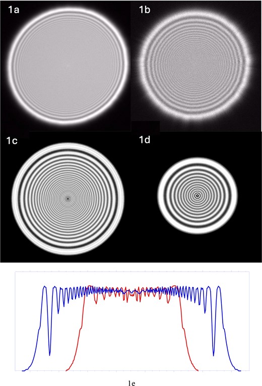
Experimental (a,b) and calculated (c,d) Fresnel Fringe Images of Illumination probe for large (a,c) to small spot sizes (b,d). Note that the magnitude, periodicity and width of the Fresnel fringes changing as shown in the line profiles (1e) across the diameters of Figs. 1c & 1d.

Open in new tabDownload slide

Fig.

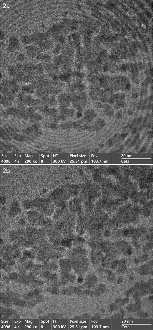
Experimental variation of contrast in CTEM imaging with FFIM mode Off (2a) and On (2b). Note the reduction of the superimposed Fresnel illumination contrast and the negligible effect on the local image contrast. E_o: 300 kV, i_o ∼ 100 pA , C₂ aperture 100 um, Magnifications as indicated.

Open in new tabDownload slide

Fig.

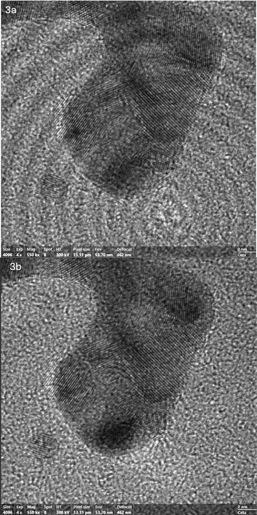
Experimental variation of contrast in HREM imaging with FFIM mode Off (3a) and On (3b). Note the reduction of the superimposed Fresnel illumination contrast and the negligible effect on the local image contrast. E_o: 300 kV, i_o ∼ 100 pA , C₂ aperture 100 um, Magnifications as indicated.

Open in new tabDownload slide

References