


Abstract
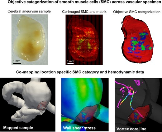
Deviation of blood flow from an optimal range is known to be associated with the initiation and progression of vascular pathologies. Important open questions remain about how the abnormal flow drives specific wall changes in pathologies such as cerebral aneurysms where the flow is highly heterogeneous and complex. This knowledge gap precludes the clinical use of readily available flow data to predict outcomes and improve treatment of these diseases. As both flow and the pathological wall changes are spatially heterogeneous, a crucial requirement for progress in this area is a methodology for acquiring and comapping local vascular wall biology data with local hemodynamic data. Here, we developed an imaging pipeline to address this pressing need. A protocol that employs scanning multiphoton microscopy was developed to obtain three-dimensional (3D) datasets for smooth muscle actin, collagen, and elastin in intact vascular specimens. A cluster analysis was introduced to objectively categorize the smooth muscle cells (SMC) across the vascular specimen based on SMC actin density. Finally, direct quantitative comparison of local flow and wall biology in 3D intact specimens was achieved by comapping both heterogeneous SMC data and wall thickness to patient-specific hemodynamic results.
Introduction
It has been well established that deviations in the quantitative and qualitative features of blood flow from an optimal range are associated with the development and progression of vascular diseases such as atherosclerosis and cerebral aneurysms (Chiu & Chien, 2011; Samady et al., 2011; Gimbrone & García-Cardeña, 2013; Frösen et al., 2019). However, these diseases involve complex changes to multiple wall components and fundamental open questions remain regarding how flow features are directly coupled to even commonly seen pathological changes such as inflammation, apoptosis of smooth muscle cells (SMCs), fibrosis, and formation of atherosclerotic plaques. If the relationship between flow and pathological wall changes were better understood, it would be possible to improve diagnosis and design more effective treatments for numerous diseases. For example, flow metrics for patients with brain aneurysms are readily available from image-based flow studies and are believed to have great potential to improve assessment of rupture risk and to guide endovascular therapies (Chung & Cebral, 2015; Rayz & Cohen-Gadol, 2020). The lack of understanding as to how the abnormal flow in the aneurysm is related to degenerative wall changes precludes the clinical use of this data (Rayz & Cohen-Gadol, 2020).
A central impediment to progress in this area is the lack of methodologies for directly relating local changes in vascular wall pathologies to local flow parameters (Cebral et al., 2019; Rayz & Cohen-Gadol, 2020). Current in vivo clinical imaging technology cannot provide data on cellular content within the wall, nor the state of the extracellular matrix (ECM) (e.g., collagen and elastin fibers). Rather, such data must necessarily be obtained ex vivo from harvested tissue samples (Gade et al., 2019). Diseased tissue is naturally highly spatially heterogenous and one technical challenge, even for such in vitro studies, is to obtain three-dimensional (3D) datasets with sufficient spatial resolution to capture cellular and acelluar wall components over spatial scales large enough to characterize the wall pathologies. In most prior work, “representative sections” were obtained to evaluate pathological samples. While valuable, this approach does not provide spatially comprehensive information about the wall pathology. Recently, Niemann et al. developed an approach to create 3D histological models of entire specimens from stacks of 2D sections (Niemann et al., 2021; Ruusuvuori et al., 2022). However, accurate reconstruction of 3D volumes remains an open area of research due to challenges associated with specimen distortion and loss of tissue during sectioning. Moreover, the discontinuous nature of these datasets limits the possibility of analyzing the 3D network structure the ECM, such as collagen and elastin, important features for biomechanical studies (Watton et al., 2009; Hill et al., 2012; Robertson & Watton, 2013; Teixeira et al., 2020).
In this study, we address this first technical challenge by introducing a new imaging pipeline in which intact samples are stained and imaged without any destructive sectioning. In particular, scanning multiphoton imaging along with immunofluorescent costaining are used to nondestructively coimage cellular content and ECM structure in large 3D sample volumes. Using this combination of scanning immunofluorescent multiphoton microscopy (SI-MPM), it is possible to obtain the spatial distribution of SMC as well as the elastin and collagen organization across entire intact samples, without destructive sectioning. As a result, the 3D architecture and colocalization of wall components can be determined.
A second important technical challenge is to categorize the state of the vascular pathology. For example, a seminal work on cerebral aneurysms categorized each aneurysm tissue based on the SMC density and organization within the tissue in order to rank the state of the aneurysm wall (Frösen et al., 2004). This approach was based on 2D histology and assigned a single ranked type to each specimen based on a sampling of 2D slices. In this work, we provide regional categorization of the SMCs across the entire intact specimen. In particular, we introduce an objective method (based on a cluster analysis) to analyze this distributed SMC data and generate a map of wall type across each specimen, rather than a single wall type for each specimen. Since vasculature pathologies are typically highly heterogeneous and intramural cells such as vascular SMCs have an important role, these advances have important scientific implications.
A third important technical challenge is mapping the histological datasets to the hemodynamic data. In a study of the role of flow dynamics in the early stages of cerebral aneurysm formation, Tremmel et al. introduced a methodology for comapping virtual slices of the hemodynamic flow field at arterial bifurcations to 2D histological datasets in that region (Tremmel et al., 2010). Using this approach, they were able to demonstrate that a combination of elevated wall shear stress (WSS) and WSS gradient led to degradation of the internal elastic lamina (IEL) and medial thinning (Meng et al., 2007; Tremmel et al., 2010; Hoogendoorn et al., 2020). Niemann et al. extended this methodology to 3D setting by mapping their 3D reconstructed histology data to 3D hemodynamic datasets, though the above-mentioned artifacts associated with this destructive approach remain. Our group previously developed a pipeline to comap flow parameters and multiphoton data for intact specimens including collagen fiber architecture, wall thickness, and calcification (Cebral et al., 2016, 2018). Here, we have extended that work to include data on SMC content while also expanding the field of view (FoV) to the order of centimeters using scanning MPM techniques.
Taken together, the methods introduced here make it possible to perform scientific studies to analyze the relationship between local hemodynamics, SMC content, ECM, and wall thickness. The state of the intramural cells and ECM are important as determining factors for the mechanical behavior of the wall, capacity for structural maintenance, and, as a result, resistance to soft tissue failure. Hence, this work has important implications for diseases such as aortic dissection, cerebral aneurysms, and atherosclerosis.
Materials and Methods
Acquisition of Vascular Specimens
For validation studies, a circle of Willis (CoW) was obtained at autopsy from a 65-year-old male (Brain Bank of the University of Pittsburgh). The right middle cerebral artery (MCA) with perforators was resected from the CoW and fixed within 24 h in 4% paraformaldehyde. The CoW had no obvious atherosclerosis. Specimen harvest and handling followed a protocol approved by the Committee for Oversight of Research and Clinical Training Involving Decedents at the University of Pittsburgh.
Specimens from four cerebral aneurysm domes were harvested during open brain surgery following surgical clipping in consented patients being treated for ruptured (n = 1) and unruptured (n = 3) aneurysms at the University of Illinois at Chicago (Chicago, IL) and Allegheny General Hospital (Pittsburgh, PA). Harvested specimens were placed in vials of HypoThermosol (Biolife, Bothell, WA, USA) transported to the University of Pittsburgh in an insulated cooler where they were fixed within 24 h of harvest in 4% paraformaldehyde. Intra-operative videos were also provided. The basic clinical information of age, sex, size, location, comorbidities, and rupture status were collected (Table 1). The average patient age was 66 ± 9 years old and the average specimen size was 5.6 ± 1.5 mm. The protocol for patient consent, handling of patient data, tissue harvest, and analysis were approved by the institutional review boards at the University of Illinois College of Medicine at Chicago, Allegheny General Hospital, and the University of Pittsburgh.
Basic Clinical Information of Aneurysm Cases.
| Case 1 | Case 2 | Case 3 | Case 4 | |
|---|---|---|---|---|
| Age | 56 | 61 | 60 | 44 |
| Sex | Female | Female | Male | Male |
| Size (Clinical) | 12 mm | 7 mm | 8.9 mm | 4 mm |
| Location | Right MCA | Right MCA | ACOM | Left MCA |
| Ruptured/Unruptured | Unruptured | Unruptured | Ruptured | Unruptured |
| Comorbidity | Hypertension | None | Hypertension | Hypertension |
MCA: middle cerebral artery; ACOM: anterior communicating artery.
Sectioned Cadaveric Specimens of Cerebral Artery: Preparation and Staining
After harvest from the CoW, the MCA artery was immersed in optimal cutting temperature (OCT) compound and snap-frozen with liquid nitrogen until OCT compound completely solidified. The embedded sample was then sectioned with cryotome (Microm HM 525 Cryostat, Thermo Scientific, Germany) at 5 μm thickness. Three sectioned slices were placed on each slide with two slices used as negative controls (NCs) for the primary and secondary antibodies, and one for full staining. Sectioned slices were twice washed for 1 min with phosphate buffer solution (PBS). The frozen sections were first thawed at room temperature and then immersed in blocking reagent [5% normal goat serum (NGS)] for 1 h at room temperature. Slides were then washed again with PBS, twice for 1 min each. Monoclonal mouse antihuman smooth muscle actin clone 1A4 IgG2a antibody (Dako, Denmark) was used as the primary antibody and Alexa Fluor 488 goat antimouse IgG2a (Invitrogen, USA) for the secondary antibody. Primary antibody was diluted to a concentration of 1% with a 1% NGS staining buffer. NC and staining samples were stained with primary antibody solution for 45 min at room temperature. Stained slides were washed again with PBS, twice with 1 min each. For secondary antibody, the solution was diluted to 1:100 ratio with 1% NGS. NCs for the secondary antibody and the staining sample were stained for 1 h at room temperature. The slide was then washed with PBS, twice for 1 min each and mounted with a mounting medium.
Whole Mount Specimens: Preparation and Staining
Cerebral artery and aneurysm specimens that were used for whole mount analysis were washed with PBS, twice for 1 min each. The entire sample was then immersed into the same alpha smooth muscle actin (αSMA) primary antibody used for sectioned tissue, for 6 h at room temperature in the dark. The sample was then washed with PBS twice for 4 min each. Secondary antibody staining was performed for 3 h at room temperature in the dark with the same secondary antibody as the sectioned specimens. Between staining, samples were thoroughly washed with PBS for 5 min.
Imaging with Confocal Microscope
Intact specimens of artery were scanned using a confocal microscope (CFM; Nikon A1, Tokyo, Japan) with a lens magnification of 20×, an NA of 0.75 and a FoV of 500 μm × 500 μm. The laser emission wavelengths were 450 nm for channel 1 and 525 nm for channel 2. Excitation frequencies were 405 nm for channel 1 and 488 nm for channel 2. Scanned images were reconstructed with IMARIS 9.5.0 (BitPlane AG, Zurich, Switzerland).
Imaging with Scanning Multiphoton Microscope
A scanning multiphoton microscope (Nikon A1R MP HD, Tokyo, Japan) with the Nikon Ni-E upright motorized system and Chameleon Laser vision was used for large area scans of the artery and aneurysm specimens as well as for 500 μm × 500 μm scans of sectioned artery tissue (scanning feature not used). An APO LWD 25 × water immersion objective lens with NA of 1.10 was used. The laser emission wavelength was set to 830 nm and the excitation frequencies were 400–492 nm for channel 1 and 500–550 nm for channel 2. For aneurysm and perforator artery scans, the large image scanning function was used with resonant scanning mode. A nano-drive system was used to acquire high-speed control of Z-plane selection. Scanned images were reconstructed with IMARIS 9.5.0 (BitPlane AG, Zurich, Switzerland). Virtual slices in the XZ-plane and YZ-plane (orthogonal to XY projected Z stacks) were cut from the 3D reconstruction images with a thickness of 10 μm.
Creation of In Silico (Virtual) Model of Harvested Specimen and Thickness Maps
Micro-computed tomography (micro-CT) scans were conducted on fixed specimens using previously reported methods and the datasets were used to create in silico (virtual) 3D models of the samples and corresponding wall thickness maps (Gade et al., 2019). Briefly, micro-CT scanning was performed using a high-resolution scanner (Skyscan 1272, Bruker Micro-CT, Kontich, Belgium) at a resolution of at least 3 μm. Virtual models of aneurysm samples were reconstructed from the Z stacks of micro-CT data (NRecon, Bruker Micro-CT, Kontich, Belgium). Wall thickness maps for each 3D virtual model were obtained using Materialize 3-matic (Materialize GmbH, Munich, Germany).
Wall Classification based on SMC Actin Density
A cluster analysis was adapted to identify subregions within 2D projections of the 3D SMC actin MPM datasets based on SMC actin density. Here, subregions with high, medium, and low-density SMC actin were defined as Types 1, 2, and 3, respectively (Fig. 1). The raw SMC actin images (Fig. 1a) were scaled down by a factor of 2, to speed up the evaluation. In Step 1, the 2D region occupied by the tissue specimen, Figure 1b (denoted with the symbol R) within the entire projected SMC actin dataset was identified using thresholding (to remove the dark background), shown as the yellow bordered region in Figure 1c. In Step 2, subregions “devoid” of SMC actin were defined by color intensities lower than 20% of the brightest pixel visible within the entire tissue region (Fig. 1d). The union of all such subregions was denoted by R0. Type I subregions were then identified using the DB.Sc.an clustering algorithm (Ester et al., 1996) which we previously implemented in Ramezanpour et al. (2023). In particular, in Step 3, high-density regions within the sample were obtained by applying the clustering algorithm to the remaining region (R–R0) using a density threshold of 12/7 (Fig. 1e). Here, the numerator corresponds to the number of pixels, and the denominator represents the neighborhood radius of the DB.Sc.an algorithm. The black cross markers in Figure 1f show pixels that are identified as noise by the clustering algorithm. 2D surfaces were then fit to the selected pixels in this step by implementing the 2D triangulation algorithm (Fig. 1f). In Step 4, the Type 1 regions (collectively defined as region R1, shown in green in Fig. 1g) were extracted by applying an area threshold of 400 (squared unit of pixels length scale) to these 2D regions (Fig. 1h). The blue regions were excluded by surface area-based filtration (Fig 1i). In Step 5, the same procedure described in Steps 3 and 4 was applied to the remaining region (R–R0–R1) with a density threshold of 7/10 and area threshold of 2,000 (squared unit of pixels length scale) to extract the Type 2 regions, collectively occupying region R2. In Step 6, the Type 3 regions were then defined as the remaining regions (R3 = R–R1–R2), containing the low-density SMC actin and regions identified as devoid of SMC actin (R0). Color maps of the three wall types could then be created for each specimen (Fig. 1j). The relative area of each wall type could then be measured and used for sample quantification purposes.
![Methodology to classify wall regions based on SMC actin clustering. Step 1: The imaging regions from Ch1 and Ch2 [shown in (a) and (b), respectively] were used to define the specimen boundary (yellow) of the specimen—region R (c). Step 2: Identify regions “devoid” of SMC. Implementing the thresholding method, pixels with color intensities less than 20% of the brightest pixel were labeled as R0 [gray in (d)]. Step 3: Using the DBScan clustering algorithm with a density threshold of 12/7 (number of neighborhood pixels/neighborhood radius), the densely distributed pixels within R–R0 were identified (e) and combined into 2D regions (filled) using the triangulation algorithm as depicted in (f). Step 4: An area threshold of 400 was applied to filter out the small 2D “islands” [shown in blue in (g)] and select the large ones (g). The union of large regions represents the high-density SMC actin regions and is defined as R1. Step 5: Using parameter values for moderate density SMC actin (7/10), the clustering algorithm of Step 3 was applied to R–R0–R1 [dots in (h)] to select pixels regions of medium density [all regions in (i) except the large regions specified in (g)]. Then, following Step 4 with an area threshold of 2,000 (squared unit of pixels length scale) the sufficiently large medium-density regions were extracted and defined as R2 in (j). Step 6: The pixels that are neither high-density nor medium-density are categorized as low-density regions [remaining area in (j)], R3 = R–R1–R2.](https://oup.silverchair-cdn.com/oup/backfile/Content_public/Journal/mam/30/2/10.1093_mam_ozae025/1/m_ozae025f1.jpeg?Expires=1750865923&Signature=ysqgRhye7tiM4EXh5zoGda1pro5L7BaqKO-nj00JImlAGbrEadsX1izB-mWZAI5atdGt0w1Sqo1BA-0D6kEtxsxWaD~W-cLPH8llVWOBcyc8T6flw96mT~nPZy5Kd1M4aR1BiYLk6ZGVUR2l0x2oM2pW6Qw~OMY11j0IX2T1RX8TJ8YW7H0ICXFYkIKbubx1IX~yTtO1GeOOqaS~rjRD60ErYkNWW2KsRXOSdLkqMvxIIONz7Y1GQ~d0gFlVGi-EBWHEps1UQYdUqm~VUvcp-7VbZ2hVO62pogC-Bip7HBG9y1o~hXzj06nBayUCq~VK0DkWzPM-1GMtjjjkFlkaig__&Key-Pair-Id=APKAIE5G5CRDK6RD3PGA)
Methodology to classify wall regions based on SMC actin clustering. Step 1: The imaging regions from Ch1 and Ch2 [shown in (a) and (b), respectively] were used to define the specimen boundary (yellow) of the specimen—region R (c). Step 2: Identify regions “devoid” of SMC. Implementing the thresholding method, pixels with color intensities less than 20% of the brightest pixel were labeled as R0 [gray in (d)]. Step 3: Using the DBScan clustering algorithm with a density threshold of 12/7 (number of neighborhood pixels/neighborhood radius), the densely distributed pixels within R–R0 were identified (e) and combined into 2D regions (filled) using the triangulation algorithm as depicted in (f). Step 4: An area threshold of 400 was applied to filter out the small 2D “islands” [shown in blue in (g)] and select the large ones (g). The union of large regions represents the high-density SMC actin regions and is defined as R1. Step 5: Using parameter values for moderate density SMC actin (7/10), the clustering algorithm of Step 3 was applied to R–R0–R1 [dots in (h)] to select pixels regions of medium density [all regions in (i) except the large regions specified in (g)]. Then, following Step 4 with an area threshold of 2,000 (squared unit of pixels length scale) the sufficiently large medium-density regions were extracted and defined as R2 in (j). Step 6: The pixels that are neither high-density nor medium-density are categorized as low-density regions [remaining area in (j)], R3 = R–R1–R2.
Mapping SI-MPM Data to Specimen Model
Prior to comapping the SMC actin and hemodynamic data, it was necessary to map the SMC actin data to a 3D reconstructed virtual model of the harvested specimen (above), for registration purposes (ParaView 5.11.0, Kitware). First, the 2D SMC actin wall type data (png file) was resampled to reduce the resolution by 50% using the ResampleToImage filter in ParaView. A planar surface mesh was created to obtain a 1–1 mapping between mesh location and wall type using the ExtractSurface filter. This mesh and associated data were then projected to the lumen side of the 3D virtual model of the specimen using the PointDatasetInterpolator filter. In Paraview, we used an Ellipsoidal Gaussian Kernel. Radius and sharpness were adjusted depending on the sample until the entire image was projected to the 3D virtual model of the specimen. Normal vectors option was enabled. All three colors were then merged into a single “color” map on the lumen side of the model providing a map between SMC actin wall type and surface position on the lumen of the virtual model of the specimen.
Computational Fluid Dynamics Simulations of Blood Flow and Associated Hemodynamic Parameters
Computational models for the 3D fluid domain were constructed from presurgical 3D rotational angiography images of the lumen of the aneurysm and neighboring vasculature using previously described techniques (Cebral et al., 2005). Blood was modeled as incompressible, constant viscosity (Newtonian) fluid with density ρ = 1.0 g/cm3 and viscosity μ = 0.04 Poise. Wall compliance was neglected, and no-slip boundary conditions were prescribed for the walls (Painter et al., 2006). Pulsatile inflow boundary conditions were prescribed using flow waveforms measured in healthy subjects and scaled with a power law of the area of the inflow vessel. The split of the outflow was chosen to be consistent with Murray's law and prescribed at the outlets. Periodic solutions to the coupled 3D system of nonlinear governing equations for unsteady flow of a Newtonian fluid (Navier–Stokes equations) and associated boundary conditions were solved numerically using finite elements with in-house software. Volumetric meshes composed of tetrahedral elements with a minimum resolution of 0.2 mm are generated filling the intravascular space using an advancing front method. Simulations were performed for two cardiac cycles with a timestep of 0.01 s, and results for pressure and velocity fields from the second cycle were saved for analysis. The velocity fields were used to calculate other previously defined field variables including the vortex core line and swirling flow around the vortex core lines (Greg Byrne, 2013; Byrne et al., 2014). Critical points within the WSS vector field across the cardiac cycle were detected, counted, and averaged over the cardiac cycle. These critical points are defined mathematically as locations on the aneurysm sac where the shear stress vector becomes zero (Seyedeh Fatemeh Salimi et al., 2021). The different types of critical points, such as saddle points, node sources or sinks, and focus sources or sinks, can be differentiated based on the local derivatives around these stationary points (Seyedeh Fatemeh Salimi et al., 2021).
Results
SI-MPM Imaging Captures Autofluorescing and Immunofluorescing Signals More Effectively Than CFM
Capturing the 3D nature of the ECM structure along with cellular contents in arterial tissues requires an appropriate whole mount staining protocol coupled with a 3D imaging modality with the capacity to image large areas with moderate or high imaging depth. To accomplish this, we applied immunofluorescent staining to whole samples and imaged them with the scanning multiphoton microscope. Here, we identify SMC by staining actin filaments within SMCs (αSMA). In addition to the conventional Z moving stage, the scanning multiphoton microscope has an XY moving stage, making it possible to capture immunofluorescent and/or autofluorescent signals over a larger area, equivalent to that possible with a ribbon CFM, while maintaining the imaging depth of MPM.
First, we illustrated the capacity for stacking autofluorescing and immunofluorescing signals obtained from scanning MPM of arterial specimens without interference. A cerebral artery from a cadaver was cryosectioned, immunostained, and scanned to assess the capability of MPM for coimaging collagen, elastin, and SMC in 2D sections (Fig. 2a). Using MPM, it was possible to clearly image the autofluorescing signal from collagen fibers in Channel 1 (i) and from the IEL in Channel 2 (Fig. 2a-ii). The adventitial collagen has a higher signal intensity than the medial collagen (Fig. 2a-i). The immunostained SMC actin was visible in Channel 2 (Fig. 2a-ii). The stacked image (Fig. 2a-iii) confirms both collagen and SMC actin are uniquely fluorescing in each channel and can therefore be distinguished. The thick IEL was present in both channels (white arrow in Fig. 2a-i, ii) and yellow in the stacked image (Fig. 2a-iii).

Multiphoton microscope can stack autofluorescing and immunofluorescing signals without interference. (a) Demonstration of stacking of autofluorescing (collagen, elastin) and immunofluorescing (SMC actin) in 2D sections. Collagen (i) and SMC actin (ii) are also observed independently when stacked using MPM (iii). As expected, IEL (arrows) is present in both Ch 1 (i) and Ch 2 (ii) as well as the combined channels (iii). The stacked image (aiii) confirms both collagen and SMC actin are uniquely fluorescing in each channel and can therefore be distinguished. (b) Demonstration of successful imaging of intact artery (3D) and superior imaging using SI-MPM versus CFM (video displaying 3D nature of data shown in Supplementary Fig. 1). In row 1, 3D rendered model of CFM (i, ii) only displays SMC actin, while SI-MPM images (iii, iv) show both collagen structure and SMC actin. Virtual slice (iv) shows SI-MPM imaging through cross-section with greater depth and clarity compared with CFM (iv versus ii). The Z projection images of each channel are shown in v to xvi. As expected, CFM of NC without SMC actin staining (v, vi, vii) sample does not fluoresce any signals, whereas SI-MPM shows autofluorescing for both the collagen structure (xi), and IEL (xii) in high detail. With staining, the aligned SMC actin in the artery is clearly captured in both CFM (ix) and SI-MPM (xv). However, the depiction of SMC in CFM has less clarity than in SI-MPM. (c) By modifying the threshold and contrast for Ch2, the dimmer elastin signal and SMC actin signal were both visible in an SI-MPM virtual slice (XZ-plane).
Second, we evaluated the ability of MPM to capture both autofluorescing and immunofluorescing signals in 3D with equivalent or higher quality than the conventional CFM. In Figures 2b and 3d, scans using CFM and SI-MPM on neighboring cylindrical sections of a small perforating artery from a MCA were compared. For the CFM, the FoV of CFM was 500 μm × 500 μm and imaging depth was 120 μm. In contrast, for the SI-MPM, the entire surface of the sample could be scanned to cover an imaging area of FoV of 4,340 μm × 1,045 μm with an imaging depth of 914 μm (Fig. 2b-iii). A movie showing the 3D rendered vasculature with a close-up of collagen signals and SMC actin signals are shown in Supplementary Figure 1 (video) to further illustrate the high resolution, comprehensive, and 3D nature of this SI-MPM dataset. To compare a SI-MPM image with similar area and magnification to that of confocal, a virtual slice was taken from a 500 μm × 500 μm region of the SI-MPM data (Fig. 2b-iii, white dotted region). A comparison of Figure 2b-ii and iv shows SI-MPM imaging through cross-section with greater depth and clarity compared with CFM. The Z projection images for both CFM and SI-MPM were also analyzed. As a reference, the NC for αSMA in the first column, showed no SMC actin under CFM for any channel (Fig. 2b-v, vi, vii). Similarly, the NC of SI-MPM in the third column did not show any SMC actin signal, though both the autofluorescing collagen fibers (Fig. 2b-xi) and the undulations of the IEL (Fig. 2b-xii) were visible (not possible under CFM). The autofluorescing collagen signal was still successfully captured by SI-MPM in the stained sample (Fig. 2b-xiv). While the SMC actin were visible in Channel 2 under CFM (Fig. 2b-ix) and SI-MPM (Fig. 2b-xv), the SMC actin in CFM showed less clarity than under SI-MPM (Fig. 2b-ix versus xv). In the SI-MPM images it was even possible to identify the circumferentially aligned SMC actin in the artery (Fig. 2b-xv). Stacked images (Fig. 2b-xvi) show the SI-MPM successfully captured both the immunofluorescent signal of SMC actin (green) and autofluorescent signal for collagen (red) independently, as was possible for the 2D sample. For SI-MPM, by adjusting the threshold and contrast of Ch 2, it was possible to visualize SMC actin and IEL, individually or collectively. In particular, the signal from elastin was clearly visible when the thresholding and contrast were adjusted to include lower intensity signals (Fig. 2c, dim green).
SI-MPM Can Coimage SMC Actin and Collagen in High Detail Throughout the Volume of Thin, Intact Pathological Arterial Specimens
The ECM of pathological tissues can differ from nonpathological arteries affecting, for example, the types and density of collagen fibers, which can in turn influence the quality of MPM imaging (Robertson et al., 2015). We therefore evaluated the SI-MPM protocol in pathological arterial tissues. In particular, we imaged two cerebral aneurysm samples with different wall thicknesses. Case 2 (Fig. 3a) had a maximum wall thickness of 270 μm with an average wall thickness of 97 ± 56 μm (i, sample size ∼2 × 3 mm) based on the 3D reconstruction of micro-CT scan of the tissue sample (Fig. 3-i). SMC actin (Fig. 3a-iii) was found over a majority of the sample, though small regions lacked SMC actin. A virtual slice in the orthogonal plane (region of virtual slice denoted by dashed lines in Fig. 3a-iii) demonstrated MPM was capable of imaging through the entire thickness of this sample (Fig. 3a-iv and v). Further, SI-MPM captured the heterogeneity of the collagen structure and density across 3D volume. In the Z projection (Fig. 3a-ii), the heterogeneity in collagen signal intensity can be seen in the lower half of the image. In the virtual XZ slice, regions of sparse collagen can be seen at the center of the wall (Fig. 3a-iv).
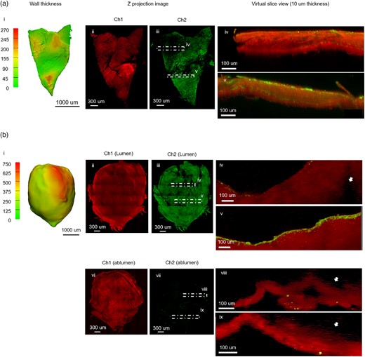
SI-MPM captures the detail of collagen and SMC actin across volume in thin samples Column 1 displays wall thickness maps for each specimen, created from 3D reconstructed micro-CT data. Remaining columns show data from large area MPM scans. (a) For aneurysm Case 2, the maximum wall thickness is 270 μm (i). The Z projection of Ch1 (ii) displays the heterogeneity in collagen signal intensity across the sample. The Z projection image of SMC actin (iii) shows heterogeneity in SMC actin density. Virtual XZ slices for stacked channels (10 μm thickness) are shown for regions of low (iv) and high (v) density SMC actin signal in Ch2. The SMC actin signal can be seen across the thickness in high-density region (v). (b) In contrast, aneurysm Case 4 is a thick sample (i) with regions that exceed the imaging depth of MPM and was therefore scanned from both luminal and abluminal sides. Z projections of both scans display detailed collagen fiber network (ii). In the orthogonal view seen in virtual XY slices (in iii: iv, v) and (in vii: viii, ix) the end of visible region from each imaging direction can be seen (arrows). Lumen is up in all images. Virtual slices from poor (iv) and rich (v) SMC actin regions show that SMC actin localized near the lumen surface in both regions.
The average wall thickness of Case 4 was 549 ± 279 μm and was 750 μm in the thickest region (Fig. 3b-i). Though the entire projected area could be imaged, it was not possible to image through the entire thickness. Therefore, scans were performed from both luminal and abluminal sides. From the lumen side, the collagen appeared amorphous (Fig. 3b-ii) rather than as the distinct collagen fibers that were seen in the thin sample (Fig. 3a-ii). SMC actin was largely present across the entire sample (Fig. 3b-iii) with only a few spots lacking signal. The region-dependent absence of SMC actin was also seen in a virtual slice at location iv (Fig. 3b-iv). As previously noted, the sample thickness exceeded the imaging depth of the microscope and as a consequence the collagen signal was lost within the tissue (Fig. 3b-iv, white arrow). In a virtual slice at location v in Figure 3b-iii, the SMC actin signal was seen to be concentrated just below the lumen (Fig. 3b-v). When imaged from the abluminal side, a complex network of collagen fibers was seen across the sample (Fig. 3b-vi), whereas the SMC actin signal was largely absent (Fig. 3b-vii). Virtual XZ slices at location iii and iv in Figure 3b-vii, both showed loss of signal beyond 100 μm when imaged from the albumen side (Fig. 3b-viii, ix, white arrow).
Use of SI-MPM Images for Computational Pathology
An important consideration in analysis of microscopy data is development of protocols that provide objective quantitative and categorical results, avoiding user bias and speeding analysis. Here, we developed an automated cluster analysis for the Z projection of SMC actin data in order to objectively categorize regions of different SMC actin type across pathological samples. In particular, three wall categories were introduced based on SMC actin density (Fig. 4a). Types 1, 2, and 3 regions had high, moderate, and low density, respectively. The wall typing was illustrated in four aneurysm specimens (Fig. 4b) and the distribution of types across each sample was analyzed from these data (Fig. 4c). SMC actin type was heterogeneous within and between samples. For example, the majority of the aneurysm sample for Case 1 lacked SMC actin signal (Type 3), while the central region was well endowed with SMC actin (Type 1 and Type 2) (Figs. 4b-i, v and 4c-i). Aneurysm tissue for Case 2 was predominantly Type 1, though it displayed all three wall types (Figs. 4b-ii, vi and 4c-ii). The Type 1 region was separated into two subregions by an interface with low or moderate density SMC actin. Case 3 aneurysm sample was dominated by regions with either moderate or low-density SMC actin (Figs. 4b-iii, vii and 4c-iii). In contrast, the aneurysm from Case 4 was endowed with rich levels of SMC actin across 93% of the sample, with small scattered Type 3 areas (Figs. 4b-iv, viii and 4c-iv).
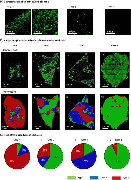
Demonstration of cluster analysis on SI-MPM images to objectively characterize regions of SMC actin density (a) Categories of wall region based on SMC actin density. Types 1, 2, and 3 correspond to high, moderate, and low density of SMC actin signal, respectively. (b) Cluster analysis was used to objectively identify regions of each SMC actin wall type in four cerebral aneurysm samples (Cases 1–4). In row 1 (i, ii, iii, iv), regions of each wall type are outlined in Z projections from Ch2. In row 2 (v, vi, vii, viii), the regions are filled with pseudo colors. (c) Post processing of cluster analysis results shown in (b) enable quantitative comparisons between samples, such as the ratio of area fraction of each SMC actin type for the four cases (ix, x, xi, xii).
Mapping SI-MPM Data to Vascular Models for Studies of the Role of Hemodynamics in Wall Pathology
To determine the possible role of abnormal hemodynamics on pathological changes in the vascular wall, it is essential to comap wall pathology data with hemodynamic data. Here, we introduce a methodology to comap the SI-MPM biological data to flow results obtained from computational fluid dynamics (CFD) simulations, performed using the corresponding patient-specific vasculature. This approach was demonstrated for Cases 1–3 (Figs. 5–7) where sufficient clinical data were available to map the harvested tissue back to the vasculature model. Below, the methodology and corresponding analysis are described in detail for these cases. Briefly, to comap these datasets, we first create a 3D in silico (or virtual) model of the harvested tissue sample for each case using micro-CT data. The SI-MPM data are then mapped to the in silico model which can then be mapped to the 3D vasculature. Using this approach, the wall pathology data (SMC actin type, collagen fiber orientation) can be directly related to patient-specific hemodynamic data (e.g., WSS).

Comparison of hemodynamics and local wall biology for Case 1. (a) Mapping procedure used to determine spatial relationship between harvested specimen and 3D reconstructed aneurysm. Ink mark applied during open brain surgery (i, ii, arrow) and morphological features on the parent aneurysm (triangle), shoulder of bleb (asterisk), and bleb (circle) were used as landmarks for mapping aneurysm specimen to patient-specific geometry of the aneurysm and neighboring blood vessels in Case 1 (iv). (b) Data for SMC actin wall type were mapped onto lumen side of 3D reconstructed specimen (i), shown with wall thickness map for comparison (ii). In (i), three spatial locations are denoted by A, B, C for comparing flow and wall structure in the Results section and Table 2. The virtual sample with SMC actin data is then mapped to 3D vasculature (iii). Abluminal side is outward and mapped sample is transparent to enable wall regions on lumen side to be seen. (c) Local hemodynamic data at diastole and systole were compared with SMC actin data for aneurysm specimen. SMC actin fibers were present in the thick bleb area (A) but not in the bleb shoulder and parent aneurysm (B, C, respectively). Critical points, where the WSS vector value is zero during the cardiac cycle, were all located outside of the specimen region (vii). A critical point on the back wall is projected onto the bleb. The WSS (i, v) was low in diastole and systole, both inside and outside of the bleb at the tissue region. OSI (iv) was also low across the specimen.
Summary of Analyses Results from Each Modality.
| Case 1 (Bleb, Luminal) | ||||
|---|---|---|---|---|
| Region | A | B | C | |
| SMC types | Type 1 | Type 3 | Type 3 | |
| Wall thickness | Thick | Thick | Thick | |
| WSS | Low | Low | Low | |
| OSI | Low | Low | Low | |
| Collagen | Virtual slice | Distinct/diffuse | Distinct/diffuse | Distinct/diffuse |
| Z projection | Dense | Dense | Dense | |
| – | – | – | ||
| Case 2 (Parent dome, complete scan from ablumen) | |||||
|---|---|---|---|---|---|
| Region | A | B | C | D | |
| SMC types | Type 1 | Type 1 | Type 3 | Type 3 | |
| Wall thickness | Moderate/thin | Moderate/thin | Moderate | Thin | |
| WSS | High | Moderate | High | High | |
| OSI | Low | High | Low | Low | |
| Collagen | Virtual slice | Distinct/diffuse | Distinct/diffuse | Distinct | Distinct |
| Z projection | Unidirectional | Unidirectional | Unidirectional | Unidirectional | |
| Tortuous | Straight | Straight | Straight | ||
| Case 3 (Parent dome, complete scan from ablumen) | |||||
|---|---|---|---|---|---|
| Region | A | B | C | D | |
| SMC types | Type 2 | Type 1 | Type 3 | Type 1 | |
| Wall thickness | Thin | Thin | Thin | Thin | |
| WSS | Low/moderate | Low | Low/moderate | Moderate | |
| OSI | Low | Low | Low | Low | |
| Collagen | Virtual slice | Distinct/diffuse | Distinct/diffuse | Distinct | Diffuse |
| Z projection | Bidirectional | Bidirectional | Uni and Bidirectional | Diffuse | |
| Tortuous | Tortuous | Straight/tortuous | - | ||
Case 1
The comapping methodology is first described in detail for Case 1 and other cases follow similarly. Alignment of the harvested specimen to its original position in the 3D vasculature is the most challenging aspect of this process (Fig. 5a). Access to images (for example from a surgical video) before (Fig. 5a-i) and after specimen harvest (Fig. 5a-ii) are necessary. Geometric landmarks on the physical sample that are apparent in the surgical images (A, B, C in Fig. 5a-ii) as well as markings applied to the tissue during surgery using surgical marking pens (Xodus Medical Inc.) (white arrow in Fig. 5a-i, ii) are used to determine the orientation and origin of the harvested specimen on the 3D reconstructed aneurysm. The geometric landmarks are also visible in the dissection scope image of the harvested specimen (Fig. 5a-iii, A, B, C). These markings enable the 3D in silico (or virtual) model of the harvested tissue (orange in Fig. 5a-iv) that was created from the 3D micro-CT data to be aligned on the 3D reconstructed vascular model (Fig. 5a-iv).
The wall pathology data obtained from SI-MPM (here, the 2D dataset for SMC actin density type) are projected onto the lumen face of the in silico 3D specimen model (Fig. 5b-i). Wall thickness maps for the sample (Fig. 5b-ii) can be directly compared with this pathology data either qualitatively or directly based on subregions in the virtual sample. The aneurysm specimen in Case 1, contains a bleb, or outcropping that can be seen as an extended region in Figure 5a, and is the thickest part of the sample (Fig. 5b-ii, up to 1,540 µm). Both the SMC actin data and the wall thickness data can in turn be mapped onto the vasculature (Fig. 5b-iii) based on the prior alignment shown in Figure 5a-iv. In Figure 5b-iii, the abluminal side of the in silico model is outward and made opaque so the colored regions of SMC all types are visible. As seen from a comparison of Figure 5b-i and ii, regions of SMC actin Types 1 and 2, though scattered, are found within the thickened section of the sample, corresponding to the bleb, suggesting the potential for ECM remodeling/maintenance in this region. This is consistent with the rich collagen fibers seen in the bleb region (region bounded by dashed yellow curve in Supplementary Fig. 2a-i). Both SMC and collagen fibers in this region are also apparent in the cross-section from the bleb region (Supplementary Fig. 2a-v). At the shoulder of the bleb, the SMC actin is absent (Type 3), suggesting little capacity for remodeling. Here, the collagen fibers have a diffuse appearance, suggestive of thin, immature collagen fibers (cross-section in Supplementary Fig. 2a-iv).
As a result of the mapping in Figure 5b-iii, the relationship between the mapped pathology data and patient-specific hemodynamic outcomes can be compared within the same 3D vasculature (Fig. 5c). For example, the relationship between SMC actin categories and WSS magnitude, streamlines and vortex corelines for Case 1 can be evaluated (during diastole (Fig. 5c-i, ii, and iii), and during systole (Fig. 5c-v, vi, and vii). Similarly, the effect of Oscillatory Shear Index (OSI) and the wall critical points can be considered (Fig. 5c-iv and vii). Movies of the hemodynamics throughout the cardiac cycle are available in Supplementary Figure 3 for all cases so flow indices at intermediate time points can be considered. Through this mapping, we enable a quantitative comparison of biological and flow data at a pointwise level across the vascular surface.
Case 1 sample is subjected to low OSI (Fig. 5c-iv) and uniformly low WSS (Fig. 5c-i and v) throughout the sample region, with WSS below 15 dyne/cm2, even during systole. A vortex coreline is maintained throughout the cardiac cycle (Fig. 5c-iii, vii, and Supplementary Fig. 3) and corresponding vortex streamlines are evident (Fig. 5c-ii and vi). However, the flow is quite slow in the region of the sample, with low WSS, typical of flow in large aneurysms of this kind. This environment was conducive to the wall thickening within the bleb, as described above. The critical points observed at the bleb (Fig. 5vii) are projections from the posterior aneurysm wall. Consequently, no critical points exist within the sampled region.
Case 2
In Case 2, the aneurysm specimen is derived from a distinct pink-hued tissue adjacent to the red transparent region, as illustrated in Figure 6a-ii (dotted line). Detailed information about the alignment process of the tissue is available in the Supplementary Material. The wall thickness of Case 2 was quite heterogeneous, ranging from 40 to 235 µm (Fig. 6b-ii). It is striking that there is no relationship between wall thickness and SMC type in this specimen. In particular, large expanses of thicker regions seen in Figure 6b-ii coincide with both Types 1 and 3 in the specimen (Fig. 6b-i). Notably, the Type 3 region (devoid of SMC) in the lower left quadrant in Figure 6b-i is relatively thick and well endowed with distinct, highly aligned collagen fibers (Fig. 3a-ii). The fibers are lower in density toward the middle of the sample (see, virtual slice in Fig. 3a-iv).
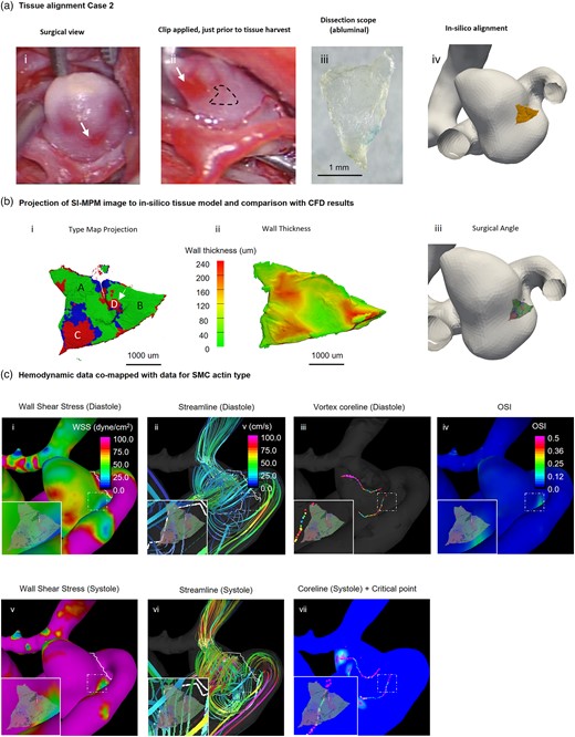
Comparison of hemodynamics and local wall biology of Case 2. Local comparison of SMC actin types and hemodynamic parameters. (a) A mapping procedure similar to that for Case 1 (Fig. 5) was used to determine the spatial relationship between the harvested specimen and the 3D reconstructed aneurysm. The dotted line in (ii) represents the location of the harvested tissue. (b) SMC actin wall type were mapped onto the lumen side of the 3D reconstructed specimen (i) and shown with a wall thickness map for comparison (ii). The sample predominantly featured Type 1 SMC actin, with a few locations of Types 2 and 3. Four regions (A, B, C, D) are denoted in i, with A and B being the left and right regions of Type 1 wall, respectively. C and D are two spatially distinct regions of Type 3 wall. The edges of Region D displayed high gradients of SMC actin and wall thickness (arrow). (c) The WSS in Region B was moderate to high approximately 50 dynes/cm2 during systole and below 20 dynes/cm2 during diastole. Regions A and C were both exposed to very high WSS of over 100 dynes/cm2 during systole (i, v). Additionally, Region B was exposed to high OSI (iv) while other regions had low OSI. A vortex core line existed behind the harvested region in both systole and diastole (iii, vii), but no critical point was observed at the site of the sample.
Case 2 sample is located downstream of a region of maximum WSS (white arrow Fig. 6c-i), as seen from the streamlines presented in Figure 6c-ii and vi. The wall in this location is exposed to supraphysiological WSS, largely in excess of 60 dyne/cm2 (Fig. 6c-i, v). Particularly interesting are the colocalizations in heterogeneities in tissue properties and flow parameters. Namely, a steep gradient in SMC actin type can be seen in Figure 6b-i, appearing as a vertical thin band (Types 2 and 3) within a sea of green (Type 1). It is also easily visible in Figure 3a-iii. This band coincides with a strip of thinner wall (Fig. 6b-ii). In addition, the band is located at the edge of a region of diminished WSS and elevated OSI (Fig. 6c-i, iv and 6c-iv, respectively), corresponding with gradients in these hemodynamic parameters, as well. Although two distinct vortices persist throughout the cardiac cycle within the lumen of the aneurysm (Fig. 6c-iii, vii, and Supplementary Fig. 3), as for Case 1, the critical points do not directly impact the specimen (Fig. 6c-vii).
Case 3
In the surgical images for Case 3, the region of the harvested specimen displays a steep gradient in color, ranging from a white appearing section of the dome (asterisk) toward the red transparent region (triangle) above it, Figure 7a-i (relative position is shifted in Fig. 7a-ii due to clipping). A comprehensive account of the tissue harvest and alignment procedures is provided in the SupplementaryMaterial. In contrast to Cases 1 and 2, the harvested tissue for Case 3 was consistently thin, with a maximum thickness of approximately 150 μm (Fig. 7b-ii). Only a small fraction of the specimen (17%) contains dense SMC actin (Fig. 4).

Comparison of hemodynamics and local wall biology of Case 3. (a) Mapping procedure used to determine spatial relationship between harvested specimen and 3D reconstructed aneurysm. Asterisk indicates the area of whitish wall and triangle indicates the edge of the transparent region in the surgical view, dissection scope view, and in silico alignment (i, ii, iii, iv). (b) Data for SMC actin wall type were mapped onto ablumen side of 3D reconstructed (i) specimen, shown with wall thickness map for comparison (ii). Asterisk and triangle represent the landmark described in a. Four regions (A, B, C, D) are denoted in i, with A being Type 2, B being Type 1 in the center of the specimen, C being Type 3 and D being a Type 1 region at the bottom right. Virtual sample with SMC actin data is then mapped to 3D vasculature (iii). The SMC actin types were directly mapped onto the vasculature to account for differences in the curvature of the vasculature geometry and the harvested sample. (c) The WSS in the sample region was at physiological levels or lower throughout the cardiac cycle. Regions A and C with sparse or nonexistent SMC actin filaments were exposed to high temporal WSS gradient (i, v). No rise in OSI, or critical point was observed in the sample region.
As for Case 2, there seems to be a relationship between gradients in thickness and gradients in SMC type. Moreover, as for Case 1, there is no direct relationship between thickness and SMC type (Fig. 7b-i, ii). Remarkably, for Case 3 we see that even thin walls can be well endowed with SMCs (Type 1, Fig. 7b-i, ii). In fact, one of the thinnest regions of this sample (lower right side of the specimen, Fig. 7b-ii) was rich in SMCs (Type 1, Fig. 7b-i) and had a region of diffuse collagen, suggesting ongoing remodeling to stabilize the wall (Supplementary Fig. 2b-i). As for Case 2, regions of diminished SMC content can display distinct, aligned collagen fibers (Supplementary Fig. 2b-iii, iv). We also see that the regions of moderate SMC coverage contain biaxial fibers (region v in Supplementary Fig. 2b-iv), suitable for bearing biaxial loads, typical of dome-like regions. This collagen structure was maintained under low WSS and low OSI, with some temporal variations in WSS (Fig. 7c-i, iv, v, and Supplementary Fig. 3).
Discussion
Complex patterns of blood flow within the cardiovascular system generate abnormal WSS fields that are known to drive pathological changes to the vascular wall (Warboys et al., 2011; Gimbrone & García-Cardeña, 2013; Cebral et al., 2019). In some diseases, such as cerebral aneurysms, both the flow and the wall pathology can be highly heterogeneous (Chung & Cebral, 2015; Rayz & Cohen-Gadol, 2020) necessitating a methodology to spatially register local cellular content in the wall to flow dynamics. In this work, we addressed this pressing need by designing a pipeline that employs SI-MPM to nondestructively obtain comprehensive 3D images of both ECM and SMC across intact vascular specimens. This framework includes a methodology to objectively analyze this cellular data using a cluster analysis, generating categorical data on SMC density across the specimen. The location-specific data on SMC density, along with wall thickness can then be mapped to patient-specific hemodynamic results enabling direct quantitative comparison of focal flow parameters and wall biology in 3D intact specimens. In this work, we focused on cerebral aneurysm tissue, though the framework can be more generally applied to other vascular tissues.
Nondestructive Analysis of SMC Content Across the Specimen
An important factor in the success of the current approach to comap flow and wall components is the nondestructive comprehensive nature of the SI-MPM imaging. Important prior work introduced a pipeline to reconstruct 3D composite models of vascular wall from serial sectioned histological datasets using machine learning algorithms to differentiate wall regions in each 2D slice (Ruusuvuori et al., 2022). However, a challenge with these datasets is the inherent physical distortion of the sections along with the requirement for fixation. The discontinuous nature of the data means that some localized heterogeneities, including calcification particles and interfaces between wall regions may be lost. Furthermore, it is difficult, if not impossible, to explore the 3D nature of the ECM, such as collagen and elastin, important features for biomechanical studies (Watton et al., 2009; Hill et al., 2012; Robertson & Watton, 2013; Teixeira et al., 2020). An advantage of this more destructive approach is that it does not suffer from limitations in imaging depth, a consideration when using SI-MPM on thicker specimens such as Sample 2 in Figure 2. A variety of optical clearing methods have been developed (Muntifering et al., 2018) that increase the imaging depth by an order of magnitude by changing the refractive index of the sample. Such approaches can be used prior to SI-MPM analysis, though some protocol-dependent tradeoffs can exist due to the clearing process, such as swelling, removal of lipids, and dehydration of the sample.
Objective Semiautomated Categorization of SMCs
A second important contribution of the present study is the introduction of a method to objectively categorize the SMCs across the vascular wall. We used a machine learning-based image segmentation algorithm to identify subregions in the 2D projected SMC actin datasets based on cluster density. This approach goes beyond simply assessing the number of SMCs per unit area. Rather we used a machine learning-based framework (DB.Sc.an clustering algorithm) to categorize SMC density across the wall. In particular, instead of solely measuring the number of bright pixels around a central pixel, our algorithm is capable of identifying discrete islands throughout the imaging dataset with consistent densities. This capability provides users with greater precision in delineating specific criteria for labeling regions as high, moderate, and low (scattered cells) density. This is illustrated in Supplementary Figure 4, where the performance of DB.Sc.an is compared with traditional density measurements.
Given the inherent susceptibility of MPM images to noise and imaging artifacts, the incorporation of a noise-aware clustering algorithm has great importance for quantitative analyses of MPM images. Moreover, unlike traditional clustering algorithms like K-Means, DB.Sc.an does not assume a specific shape for clusters and, in contrast to hierarchical clustering, it does not depend on a predefined number of clusters in the dataset.
Here we chose to use an unsupervised rather than a supervised learning approach. Supervised machine learning segmentation algorithms generally require large labeled datasets as the ground truth for training purposes and also have high computational costs associated with the training process. In contrast, the unsupervised machine learning segmentation algorithms, ranging from very simple image thresholding methods to density-based clustering algorithms such as DB.Sc.an do not require labeled datasets to be trained and are substantially faster than the supervised algorithms. For this work, an unsupervised cluster analysis algorithm was found to be effective for categorizing SMC actin density. The application of machine learning to the field of pathology is an area of growing focus as it provides a fast and repeatable means for objectively analyzing and categorizing specimens, though open challenges remain for routine clinical implementation (Abels et al., 2019). The clinical value of these algorithms has been proven in a number of applications, such as detection of metastases of lymph nodes, demonstrating the predictive capability can be higher than even clinical experts (Steiner et al., 2018).
Our classification of the SMC wall type across the vascular specimen provides a new approach that is important for pathological specimens which are typically highly heterogeneous. While the cerebral aneurysm wall has long been recognized as heterogenous (Stehbens, 1972), it is only more recently that the structural importance of this heterogeneity has been considered (Kadasi et al., 2013; Robertson et al., 2015; Cebral et al., 2016, 2017, 2018; Tobe, 2016; Gade et al., 2019; Fortunato et al., 2021). The relevance of structural heterogeneity to the rupture process is of clinical importance for a variety of vascular diseases including atherosclerosis and aneurysms. Collagen, the central load bearing component in vascular tissues is maintained by the SMC and fibroblasts (Robertson & Watton, 2013; Gomes et al., 2021). Therefore, the state of the SMC and collagen within the wall is of primary importance in determining wall strength.
In a prior, seminal work on aneurysm wall categorization, Frösen et al. identified four cerebral aneurysm wall types based on cell content and organization, ranked from A to D (Frösen et al., 2004). Type A walls have linearly organized SMC, Type B walls are thickened with disorganized SMCs. Type C and D walls are hypocellular, with Type C being thick and Type D walls being thin. A significant association was found between wall type and rupture, with increasing likelihood of rupture from A to D. One limitation in this prior work is that only a single wall type was assigned to each sample, based on analysis of a subset of histological sections. This may explain why even 42% of Type A walls were ruptured. Using the framework introduced here, it is possible to assess the state of SMC across the specimen and thereby extend the aneurysm wall classification to a local level while also eliminating the need for subjective analysis.
We did find all four wall types described in Frösen et al. (2004) in addition to other types not described by this categorization (Frösen et al., 2004). The Type 3 regions in the current study can be subdivided into Types C and D of the Frösen typing using the wall thickness data from the same intact tissue specimens (Fig. 4b). For example, the Type 3 wall in (Fig. 3) is all of Type C. However, we also found an additional wall type not included in this earlier work. Walls with nonaligned SMCs were only reported as thick in the Frösen category system (Type B). In contrast, we found nonaligned SMCs in thin and moderate thickness walls. For example, nonaligned SMCs of Type 2 can be seen in Case 2 in thin regions (Fig. 6b-i, ii). As cell alignment is a separate variable from cell density, we did not further subdivide Type 1 based on cell alignment. The relationship between density and alignment is a topic being considered as part of a larger study.
In this work, we also considered SMC actin density and wall thickness as independent variables. In fact, an important finding of this work is that SMC density and wall thickness are independent – all three wall types can be found for a range of wall thickness ranging from thin (less than 75 mm) to thick (greater than 200 mm). It is particularly striking that we can find thin walls with dense SMCs (both aligned and nonaligned). It was also striking, that even in the absence of SMC, thin-walled regions can have a distinct collagen network (Case 2). Notably, wall thickening was always due to collagen deposition, not, for example, due to atheroma.
Concurrent Mapping of CFD, SI-MPM, and Wall Thickness
Lastly, our study overcame a third technical challenge by introducing an approach for facilitating mapping of CFD with the data for SMC actin and wall thickness. This methodology enables a comprehensive local assessment of regional hemodynamics and wall biology. The specimen from Case 1 differs from the other samples in that it comes from a bleb region within the aneurysm. The bleb wall was thickened and included Types 1 and 2 regions under an extremely low WSS, low OSI flow field, with few gradients in the flow field. This correlation suggests bleb wall remodeling is possible under this type of extremely low WSS flow field, consistent with the rich collagen content in that region. Case 2 specimen was highly heterogeneous in wall thickness and SMC coverage. There was a striking correlation between regions of steep spatial gradients in flow (WSS, OSI) with gradients in wall thickness and SMC wall type. Case 3 specimen was subjected to low WSS and low OSI, with modest temporal gradients in these flow parameters. Walls of this specimen were thin and largely of Types 2 and 3. Surprisingly, wall regions with sparse SMCs (Type 3) could be well endowed with distinct unidirectional collagen fibers. This was seen for both Cases 2 and 3. Regions of bidirectional fibers were also found associated with Type 1 walls. Conclusions about flow and wall remodeling will be considered under a more extensive study with larger numbers of samples as multiple anormal flow types are expected to have distinct and complex effects on the aneurysm wall.
Summary
Here we developed a new imaging pipeline which enables direct quantitative comparison of local flow and wall biology in 3D intact specimens. This pipeline is a substantial step forward from methods using 2D histological data that are limited by the artifacts associated with the destructive nature of serial sectioning. By using scanning MPM-coupled with immunofluorescent protocols, we obtained 3D datasets for both cellular and ECM from intact vascular specimens. These data were then mapped to 3D patient-specific hemodynamics data for direct quantitative comparison. The methodology introduced in this work makes it possible to address open questions about how local flow abnormalities drive specific wall changes in arterial diseases. This same approach can be applied to other cells (e.g., endothelial cells, inflammatory cells) as well as other biomechanical field variables such as intramural stress parameters and even geometric parameters such as local wall curvature.
Availability of Data and Materials
The authors have declared that no datasets apply for this piece.
Supplementary Material
To view supplementary material for this article, please visit https://doi.org/10.1093/mam/ozae025 .
Acknowledgments
We acknowledge the brain bank of the University of Pittsburgh for the cerebral arteries used in this work. We thank R. Fortunato (Department of Mechanical Engineering and Materials Science, University of Pittsburgh) and F. Mut for their advice on mapping the in silico models of tissue specimens to the hemodynamic models.
Author Contributions Statement
Y.T. and A.M.R. conceived and designed the project. Y.T. performed all imaging experiments and analysis of the associated datasets. S.C.W. provided expertise on the MPM studies. Y.T. and A.M.R. wrote the majority of the manuscript. M.R. developed and implemented the image segmentation algorithm for the clustering analysis of the SMC. M.R. wrote the corresponding parts of the Methods section and associated figures. F.T.C., S.A.-H., and A.K.Y. performed surgeries and harvested aneurysm specimens. J.R.C. designed and performed the CFD studies and prepared the associated figures. All authors reviewed the manuscript.
Financial Support
The authors acknowledge support for this work from the National Institution of Neurological Disorders and Stroke of the National Institutes of Health through grant 2R01NS097457 and 1S10OD025041.
References
Author notes
Conflict of Interest: The authors declare that they have no competing interest.
