Enlarged Field of View in Spatially Modulated Selective Volume Illumination Microscopy Open Access

Abstract

Introduction

Imaging large samples at the cellular level is a necessary condition in understanding the organ's anatomy and functions. To this extent, light diffusion is one of the fundamental limits in the study of biological samples. A possible solution to this problem is the usage of ex vivo chemical clearing. The procedure reduces the sample scattering by homogenizing its refraction index, allowing light to propagate without diffusing for several millimeters. Different clearing techniques have been proposed in the last decade to remove light scattering while preserving the fluorescence signal, including mixtures of solvents (such as benzyl alcohol and benzyl benzoate, BABB, or dibenzyl-ether, DBE) and hydrogels (Ueda et al., 2020).

Concurrently, high-resolution imaging of large samples has been made possible by the development of optical imaging techniques. Selective Plane Illumination Microscopy (SPIM), or Light Sheet Fluorescence Microscopy (Huisken, 2004), has proven to be particularly advantageous in the study of large, chemically cleared samples (Olarte et al., 2018). In its simplest implementation, a laser beam is tightly focused on a single plane (light sheet) of a fluorescent specimen with a cylindrical lens. The fluorescence emitted is, then, collected by a wide-field microscope, positioned perpendicular to the light sheet plane. By illuminating with a thin sheet of light limits the irradiation of out-of-focus regions, and a high-resolution and optically sectioned reconstruction of the sample can be easily retrieved.

We recently proposed an alternative approach, namely spatially modulated Selective Volume Illumination Microscopy (smSVIM) (Calisesi et al., 2019). Similarly to SPIM, in this technique, the detection axis is perpendicular to the illumination direction, but without relying on single plane illumination. Instead, several planes are simultaneously illuminated by projecting a pattern modulated along the z-axis onto the sample (Figs. 1a, 1b). The specimen is kept static since its translation might be impossible or limited, due to its porous structure, or it might be misplaced by motion. For the reconstruction of the volume, the fluorescence emitted by different illumination patterns is recorded and processed by solving an inverse problem: Given N linearly independent patterns, N sections of the sample are reconstructed. This method can be implemented with incoherent light sources, such as Light Emitting Diodes (LED), making the system attractive for low-cost, shadowing free, volumetric microscopy applications. Furthermore, smSVIM can be combined with compressed sensing strategies (Candes & Wakin, 2008; Calisesi et al., 2021), reducing the number of acquisitions needed for a 3D reconstruction (Woringer et al., 2017; Calisesi et al., 2019). This can be beneficial for high-speed imaging and to lower the photodamage of the sample during the measurement.

Fig. 1.

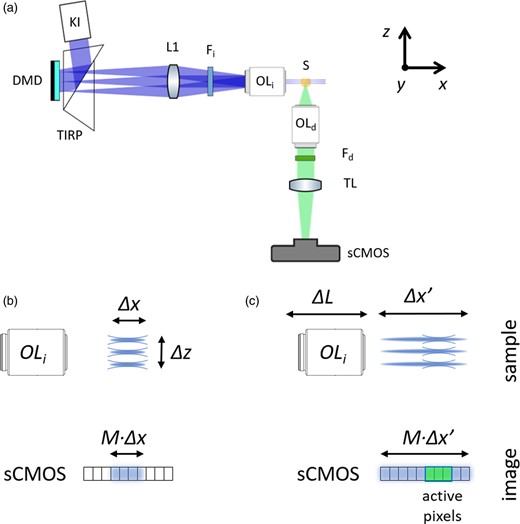
(a) Experimental setup: the light emitted from an LED is projected by a Köhler Illuminator (KI) to a Digital Micromirror Device (DMD) using a Total Internal Reflection Prism (TIRP). The light reflected by the DMD is collected by the lens L1, filtered by the illumination filter F_i and imaged on the sample (S) by the objective lens (OL_i). The fluorescence emitted by the illuminated volume is collected by the detection objective (OL_d) and the tube lens (TL), filtered by the emission filter F_d, forming an image at the camera (sCMOS). (b) The pattern remains in focus for a distance Δx. (c) The illuminations lens (OL_i) is moved along the distance ΔL in order to scan the pattern on the sample for a distance Δx. The acquisition with the rolling shutter of the sCMOS camera is synchronized with the motion of the lens OL_i, sequentially activating the pixels that correspond to the focus position of the pattern.

Open in new tabDownload slide

However, when it comes to measuring a large (chemically cleared) sample, techniques based on lateral illumination suffer two major optical disadvantages. First, the illumination objective typically has a depth of field (DOF) which is orders of magnitude shorter than the total extent of the specimen along the x-direction. Second, the detection objective has its best resolution confined within a narrow region around its focal point: the further the signal is emitted away from its DOF, the more it will degrade due to defocused detection. The goal of the present work is the development of strategies for the improvement of smSVIM imaging capabilities in both transverse and axial directions. To do this, we combine hardware and software approaches. The limited extension of the illumination pattern is effectively enlarged by synchronizing the movement of the illumination objective with a progressive activation of the camera sensor. A preprocessing deconvolution routine, on the other hand, is performed to increase the imaging quality outside the detection DOF. We speculate that each projected image acquired by the camera got blurred by an—overall effective—point spread function (PSF). We compute this PSF by projecting its defocused distribution along the entire imaged volume, and then we use it to deconvolve each camera image before their inversion. With the said approach, we enable the acquisition of mm-scaled chemically cleared tissues without the need of any sample movement and with improved imaging resolution.

Materials and Methods

Spatially Modulated Selective Volume Illumination Microscopy on a Large Field of View

The first element of the optical setup is an LED coupled to a Köhler Illuminator (Fig. 1a) to illuminate a Digital Micromirror Device (DMD). The DMD generates a pattern consisting of vertical lines (parallel to the y-axis in Fig. 1) that are projected on the sample by the illumination objective lens OL_i. The sample is placed in a cuvette and immersed in a liquid for refractive index matching. The pattern remains in focus within a distance Δx (Fig. 1b), illuminating a volume of the sample that is modulated along the z-direction. The presented schema results in an axial pattern that has spatial extension Δz, determined by the illuminated spot on the DMD and the illumination optics. Here, we use a depth Δz that is, approximately, twice the depth of field of the detection objective lens OL_d. The light emitted by the sample is then collected orthogonally by the detection objective OL_d and forms an image on the scientific complementary metal-oxide semiconductor sCMOS (camera). Thus, the collected image is the sum of the fluorescence signal originated by the different planes of the sample within the selected volume of depth Δz. We project N patterns forming a Walsh–Hadamard (WH) basis (Beer, 1981) modulated along the z-direction, and we acquire the N corresponding images consequently. For each pixel (x, y), the N amplitude values constitute the WH spectrum. The fluorescence distribution is reconstructed thanks to the fast WH inverse transform (Beer, 1981) applied in parallel to all pixels.

In order to image large biological tissues, we use low-magnification detection objective lenses, in particular 2× and 5×. This choice reduces the resolution to a few micrometers (Table 1), but it also allows to acquire larger tissues in a single scan (Voigt et al., 2019). For illumination and detection, we use two objective lenses with the same numerical aperture (NA) so that the excitation cut-off frequency (2NA/λ_i) is close to that of the detection (2NA/λ_d), where λ_i is the illumination and λ_d is the detection wavelength, respectively. However, since the incoherent light pattern remains in focus only within the illumination depth of field and the modulation shows high contrast only within a restricted extent Δx, the three-dimensional reconstruction is limited to a narrow field of view. We note that, along the y-direction, the pattern extends over a distance Δy instead, corresponding to the field of view (FOV) of the illumination objective, which is greater than Δx (see Table 1). Having the same value for Δx and Δy would be ideal for complete exploitation of the field of view of the imaging system.

To extend the field of view, we translate the illumination objective along the x-axis by translating it back and forth during the acquisition. To this purpose, we use a voice coil motor which moves the objective by a distance ΔL and, as a consequence, translates the patterns by a distance Δx′ = ΔL ⋅ n (using the paraxial approximation), where n is the refractive index of the liquid in the chamber. In this way, an effective pattern with an enhanced persistence length is created and the modulation is ultimately limited by the sensor size. However, the translation of the illumination focus would not guarantee that a high contrast pattern is created along with the entire distance Δx′ due to its diverging profile. To reject the out-of-focus contributions, we synchronize the stage motion with the camera sensor reading. We use the camera in the so-called rolling shutter mode (Baumgart & Kubitscheck, 2012; Silvestri et al., 2012; Song et al., 2016), where the columns of the sCMOS sensor are used as a slit detector. Each line of the sCMOS chip is activated sequentially and the readout is performed from one side of the sensor to the opposite. The rolling shutter is synchronized with the motion of the linear stage so that they are both triggered by a change of the DMD pattern. For our measurements, we activate a group of columns in the sCMOS, which we slide across the image sensor. This movement is synchronized with the translation of the illumination objective. The optimal number of columns being simultaneously open is, hence, determined by the illumination numerical aperture. With a highly focused excitation beam (higher NA) strong light intensity is delivered in a narrow region. Because of this, fewer columns can be kept concurrently open, reducing their exposure time. According to the desired frame exposure, the speed of the translation stage is set to cover the sample thickness in such interval of time. For the samples presented in this manuscript, a single frame exposure lasted about 1 s, as the maximum number of columns opened at once was around 350, in which a single line is kept open for 100 ms. A similar approach has been proposed by Dean et al. (2015) and is adopted in state-of-the-art SPIM systems (Voigt et al., 2019). One of the advantages of this method is to decouple the lateral (x,y) and axial (z) resolutions so that, by using the same objective lenses for illumination and detection, isotropic resolution can be potentially achieved. However, considering that the size of the DMD pixel is larger than the size of the sCMOS pixel and that the finest degree of modulation is two DMD pixels for projection, we expect the axial resolution to be three times worse than the lateral.

Setup

The light from an LED emitting either blue or red light (Thorlabs SOLIS-445C and Thorlabs SOLIS-623C) is filtered by a band pass filter (475 AF 40 and Thorlabs FB620-10) and coupled to a Köhler illuminator. By means of a total internal reflection prism (Henan Kingopt, custom made prism), the light is projected on a DMD (Texas-Instruments DLP LightCrafter 6500). The pattern created on the DMD consists of vertical lines (in the yz-plane). The pixel size of the DMD is 7.6 μm but, since the micromirrors rotate around their diagonal, the device is mounted with a tilt around its axis, giving an effective line spacing of 10.7 μm. The modulation masks are generated binning two lines together, in order to create a pattern at the sample with higher modulation contrast. The Köhler illuminator creates a uniform circle with 12 mm diameter on the DMD.

The patterns generated by the DMD consist of 128 WH functions of z. For each WH function, two complementary positive patterns have been generated and projected. This approach has been proven to give high-quality reconstructions due to its robustness to noise and CW component (Rousset et al., 2018). Nonetheless, other measurement patterns can be preferred with different modulation technology (Garbellotto & Taylor, 2018; Ren et al., 2020). The sample is immersed in water (beads) or in clearing solution (tissues) in a 2.5 cm side glass cuvette. We test two objectives both for illumination and detection: a 2× (Mitutoyo Plan Apo LWD, 0.055NA) and a 5× (Mitutoyo Plan Apo LWD, 0.14 NA). The presented configuration leads to an optical power at the DMD plane of about 70 mW for both emitting LEDs. The power at the sample depends on the illumination objective: it measures 350 mW/cm² for the 4× and 100 mW/cm² for the 2× (values are obtained by considering a uniform illumination, as for the first function of the WH basis).

The fluorescence emitted by the sample is collected orthogonally to the illumination arm, by the detection objective OL_d and then filtered by a band pass filter centered at λ_d = 520 nm or λ_d = 670 nm (Omega Filter 518QM32 and 695AF55). In combination with a tube lens (Nikon MXA20696), the objective lens OL_d forms an image at the scientific CMOS camera (Hamamatsu Orca Flash 4, 2,048 × 2,048 pixels with 6.5 μm side). The acquired image is the sum of the fluorescence signal originated by the different planes of the sample within the selected volume of depth Δz.

For the extension of the field of view along x, we use a voice coil motor (Physik Instrumente, C-413 PIMag Motion Controller, V-524 linear stage), with maximum oscillation frequency of 15 Hz. Said stage is synchronized with both the DMD and camera by a custom Python software, based on the library Scope Foundry (Durham et al., 2018).

Image Formation and Deconvolution

When imaging an object O(x, y, z) with an optical system characterized by its PSF, it is common to consider the blurring as an isoplanatic process along both xy-directions. However, the fluorescence emitted from different depths is characterized by a PSF that progressively degrades as emission comes from out-of-focus planes. In this work, we theoretically simulated the variation of the PSF along the z-direction, by considering the aberrations induced by the presence of air, glass, and clearing solution interfaces. Thus, the PSF of the presented system can be mapped as a function of the three-spatial directions, PSF(x, y, z), that blurs along the first two:

where R(x, y, z) corresponds to the volume reconstruction obtained by directly solving the smSVIM problem. The technique permits to selectively excite the fluorescence at different depths, by projecting a binary pattern that is uniform along xy and depends only on χ_i(z). Thus, each camera detection can be written as a projection of the excited volume along the z-axis:

where χ_i(z) is a step function whose values are either 0 or 1. The underlying idea consists of approximating the recorded projection as blurred by an effective PSF determined by its modulation as:

where a reasonable choice can be , which depends on the specific mask adopted. Since the smSVIM relies on the difference between the pattern modulated with χ_i(z) and its negated version 1 − χ_i(z), the WH image will be made of different blurring contributions along the z-axis. Thus, we assume that a choice for an effective PSF is the projection of the PSF map across the entire volume:

where a is a constant that we introduce to normalize the PSF, and so that:

With the formulation above, we consider each camera acquisition blurred by the same (camera isoplanatic) PSF_eff. The preprocessing step of the raw acquisitions is accomplished by deconvolving with such effective point spread function. Although this is not rigorous, we found that pre-deconvolving with the same effective PSF behaves better than either pre-deconvolving with a modulated PSF-projection and post-deconvolving the reconstruction of the smSVIM.

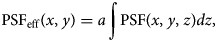
To reinterpret tomographic information based on modulated projections, the smSVIM relies on the solution of an inverse problem. Due to its experimental design, the resolution of the volume gets progressively worse when looking away from the focal plane. In simple terms, the PSF changes with the depth due to defocused contributions. In general, deconvolution approaches can be used to compensate for defocus (Berriel et al., 1983; Jayaweera et al., 2021). However, we found that deconvolving each plane with a varying PSF produces artifacts that depend on the position along z. To avoid this, we propose to uniformly enhance the image quality by interpreting the deconvolution problem as a preprocessing task, to be executed on raw data before the Hadamard inversion.

Each raw data recorded by the camera is the z-projection C_i(x, y) of the object modulated by a binary pattern χ_i(z), which turns on/off the signal emitted at different depths. It follows that every image is corrupted by a non-trivial blurring. In smSVIM, the Hadamard measurement consists in subtracting from a single pattern contribution, its negated implementation. Thus, the image used for Hadamard inversion is a linear combination of the fluorescence excited in the whole sample, modulated via a sign change along the z-axis. In this context, we approximate the image blurring with an effective point spread function projected along the z-axis as . By doing this, we can implement an iterative Richardson–Lucy (Richardson, 1972) deconvolution scheme to preprocess each camera projection as in:

where t denotes the iteration step that leads to the deconvolved image . We run 30 iterations in parallel for each projected pattern C_i(x, y). The implementation of the method was written in Python and run on a GPU Nvidia Titan RTX. For a faster execution, we used depth-wise convolution routines in PyTorch as in Ancora et al. (2021) but here, instead, using the same PSF for all the images.

Reconstruction from smSVIM Acquisition

After the deconvolution process, the images C_i(x, y) are subtracted two-by-two to recreate the correct measurement of the WH mask. In fact, the WH masks consist of ±1 values and are physically implemented with two measurements obtained by projecting two positive complementary masks. Afterward, the fast WH inverse transform (Beer, 1981) is applied to each pixel to reconstruct the volume R(x, y, z).

Mouse Brain Labeling and Tissue Clearing Protocol

Animal experiments were carried out in compliance with the institutional guidelines for the care and use of experimental animals (European Directive 2010/63/UE and the Italian law 26/2014), authorized by the Italian Ministry of Health and approved by the Animal Use and Care Committee of the University of Milan.

Adult healthy wild-type mice were cardially perfused with 30 mL of PBS followed by 40 mL of 4% PFA using a peristaltic pump. Brains were harvested, cut in half longitudinally, further fixed with 4% PFA for 2 h, dehydrated with methanol and stored at −20°C until use. Tissues were rehydrated, washed with 0.5% Tween-20 in PBS for 1 day at 4°C under agitation and incubated for 3 days with a blocking solution (10% donkey serum, 0.1% Triton-X, 0.05% Sodium Azide). Samples were then incubated with rat anti-PECAM1 (MEC13.3, BD 550274, 1:200) primary antibody diluted in blocking solution for 7 days at 4°C under agitation. Samples were washed in PBS 0.5% Tween-20 for 3 days and then were incubated with donkey anti-rat secondary antibody conjugated with Alexa Fluor 647 (Jackson Immunoresearch, 1:500) in blocking solution at 4°C for 7 days under agitation. Samples were washed in PBS 0.5% Tween-20 for 3 days before clearing. Immunolabelled tissues were cleared using a benzyl alcohol benzyl benzoate (BABB) protocol. Briefly, samples were dehydrated with methanol and then incubated for 2 h at room temperature with a solution composed by 50% BABB (benzyl alcohol/benzyl benzoate 1:2) and 50% methanol. Samples were then incubated in 100% BABB until fully cleared and stored at 4°C until acquisition.

Rat Brain Processing

The brain from an adult rat (female, 14 weeks) was extracted and fixed as in Perin et al. (2019). A coronal macroslice (2 mm thickness) was cut with a razor blade at the level of hippocampus/lateral ventricles and processed with iDISCO+, with two modifications. First, since no antibodies were used, incubation omitted block, primary and primary wash steps, and TOPRO was incubated for 4 h at 37°C before last wash sequence. Second, DBE was substituted with ethylcinnamate [as in Henning et al. (2019)] which has similar optical properties but is less aggressive in dissolving plastic and nontoxic (Bhatia et al., 2007).

Results and Discussion

Spatial Resolution and FOV Extension

To test the performances of the field of view extension method, we acquire fluorescent nanobeads (Estapor F1-XC 010) embedded in a transparent, solid gel matrix (1.5% phytagel in distilled water) contained in a Fluorinated Ethylene Propylene (FEP) tube. The beads were of an average diameter of 500 nm, with peaked emission at λ_d = 582 nm. The results of acquisition at 5× magnification are shown in Figure 2. Without the field of view extension, the beads at the image center (within Δx) are clearly visible (Fig. 2a), whereas in the left and right margins, there are fewer and larger emitters.

Fig. 2.

Reconstruction at 5× magnification of fluorescence beads. (a) Plane xy without field of view extension. (b) Plane xy with field of view extension. (c) Plane xz without field of view extension. (d) Plane xz with field of view extension. (e) Magnified detail of the green square in panel (c). (f) Magnified detail of the green square in panel (d). The green arrows indicate the same bead aggregate, visualized differently with the two modalities. Scale bar is 1 mm.

Open in new tabDownload slide

Conversely, the field of view extension (Fig. 2b) uniformly reconstructs the entire sample, with diffraction-limited resolution. By slicing the reconstructed volume in xz-planes (Fig. 2c), only bead aggregates are visible in the margins. Due to the illumination defocus, their reconstruction is severely elongated along the detection axis z and exhibits a reduced contrast. However, the motion of the excitation objective and the synchronization with the sCMOS camera solves this problem (Fig. 2d), reconstructing the beads uniformly with enhanced contrast. The highlighted rectangles in Figures 2c and 2d show a bead aggregate (green arrows) far from the central part of the image and whose reconstruction is elongated only when the field of view extension is not applied (Fig. 2e). To highlight the benefits given by the presented scheme, we have plotted the spatial profiles of point emitters (i.e., their PSF), both laterally and axially (Fig. 3). The translation motor synchronization with the sensor readout prevents the PSFs from broadening when recording away from the central imaging region, providing uniform contrast over the entire image plane. These results indicate that it is possible to extend the field of view by refocusing the illumination pattern, similarly to what adopted in SPIM microscopy, by refocusing a single light sheet (Dean et al., 2015; Voigt et al., 2019).

Fig. 3.

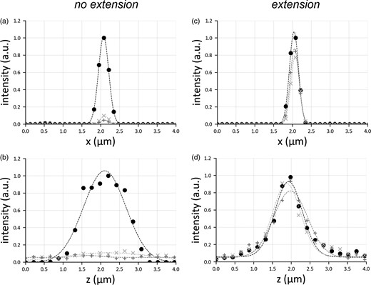
Lateral (a,c) and axial (b,d) profile of a point emitter, considering the cases in which there is no translation of the illumination objective (a,b) or in which the translation motor is used (c,d). For each panel, three graphs are shown: the circle marker represents the PSF in the center of the image, the marker “+” that at the border of the sensor, and the marker “x” shows the PSF halfway from center and border. The PSFs are all normalized with respect to the peak intensity of the emitter located at the center. Gaussian fit is added to the curve as a trendline.

Open in new tabDownload slide

Imaging of Cleared Brain Tissue

We applied our imaging strategy to chemically cleared biological samples. We labeled the mouse brain vasculature (see Materials and Methods section) with immunofluorescence for PECAM1 and acquired images at 5× magnification to reveal the capillary plexus (Fig. 4). Our imaging system yields uniform reconstructions over the entire field of view: different regions of the sample are reconstructed with similar resolutions (Fig. 4).

Fig. 4.

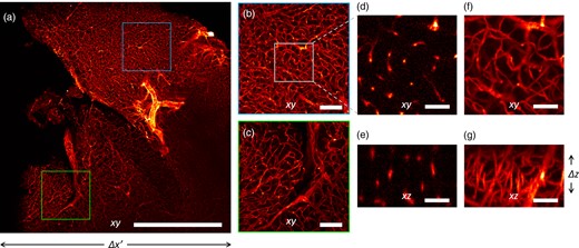
Imaging of a mouse brain at 5× magnification. (a) Maximum Intensity Projection of the reconstructed volume. (b,c) Magnified details of the blue and green boxes in panel (a), respectively. (d,f) Magnified detail of the white square in panel (b), shown in a single xy plane and as Maximum Intensity Projection, respectively. (e) Detail of the xz plane, perpendicular to the plane shown in panel (d). (g) Maximum Intensity Projection of the region shown in panel (e). Scale bar is 1 mm in (a), 250 μm in (b,c), and 40 μm in (d,g).

Open in new tabDownload slide

The three-dimensional vascular network is recovered at a lateral resolution slightly higher than the axial. The theoretical depth of field of the detection objective is 52 μm, but the reconstruction in 3D shows an acceptable blurring for at least twice the DOF (Calisesi et al., 2019). This motivates the choice of illuminating a thickness Δz, larger than the depth of field. Hence, the entire volume Δx′ ⋅ Δy ⋅ Δz is reconstructed without moving the sample.

It is worth noting that the use of LED illumination avoids shadowing artifacts typical of SPIM. Shadowing artifacts are given by the presence of scattering and absorbing centers in the sample, hindering the propagation of coherent light. This results in elongated shadows which are parallel to the light sheets. The LED source used in smSVIM effectively avoids the presence of said artifacts thanks to its broader spatial frequency support. When imaging extended samples, it is often the transport mean free path that limits the extension of the imaging region, as in several SPIM configurations. However, when using a 2× detection objective to image PECAM1 + blood vessels in an extended portion of the brain (which includes cortex, hippocampus, caudoputamen, and thalamus), smSVIM proves to be effective in recovering fluorophores distributions over a total extension of 6.6 × 6.6 mm² (Fig. 5). However, the methods found in the literature to overcome this problem include double illumination (Ding et al., 2017) and transform-based methods (Liang et al., 2016).

Fig. 5.

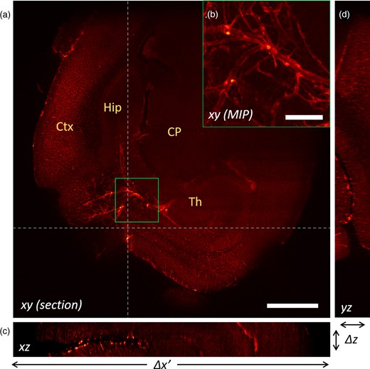
Reconstruction of a mouse brain at 2× magnification. (a) Reconstructed xy-plane of the sample. The cortex (Ctx), hippocampus (Hip), caudoputamen (CP), and thalamus (Th) are visible. (b) Maximum Intensity Projection of the detail highlighted in the green square in panel (a). The big calibre vessels likely include branches from the posterior cerebral artery, the hippocampal arteries, and veins and the thalamoperforating arteries. (c) Reconstructed xz-plane. (d) Reconstructed yz-plane. Scale bar is 1 mm in (a) and 200 μm in (b).

Open in new tabDownload slide

Nonetheless, solving an inverse problem after a modulated illumination might be troublesome. An undesired modulating factor can, in principle, generate artifacts that limit the reconstruction quality of the volume of interest. This might be the case for a nonuniform illumination spot on the DMD or sample photobleaching. While the first factor can be easily corrected, photobleaching needs an additional discussion. In fluorescence microscopy, photobleaching is a phenomenon that may occur when overexposing a fluorescent probe to light, causing an exponential decrease of the fluorescence signal over time. The described exponential modulation has also been measured in some smSVIM measurements, as in the sample presented in Figure 5. Here, together with patterned modulation, it is introduced a further factor as an exponential decay. A possible strategy to overcome this tedious problem consists of compensating for the known exponential decrease by rescaling the acquired frames by a factor I(t)/exp(−kt); with time being encoded by patterning.

Overall, the technique proves capable of acquiring a 3D volume without moving the sample and being laterally limited by the sensor size, with the possibility of further extending the depth of field (Tomer et al., 2015; Quirin et al., 2016) or scan the sample in different regions. Furthermore, reconstructions of thicker volumes might also be obtained by enlarging the modulated area at the DMD and, consequently, moving the illumination subsystem. This approach fits compressed acquisition routines which would lower the total acquisition time by an order of magnitude (Calisesi et al., 2019). In this paper, however, we investigate the reconstruction quality obtainable with a static sample by proposing a deconvolution method tailored to smSVIM.

Deconvolution of smSVIM Data

For this study, we measure a coronal macroslice extracted from a rat brain (lateral ventricle, posterior to the bregma) labeled with the TOPRO nuclear dye (Figure 6; see Materials and Methods section). We report the results obtained on the study of the cells that exhibit different nucleal sizes, in particular neuronal and glial cells.

Fig. 6.

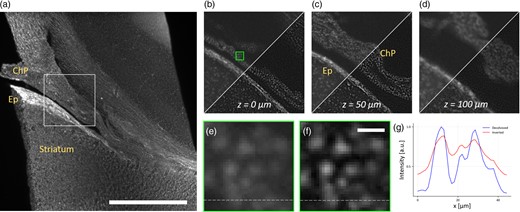
Reconstruction using the preprocessing deconvolution of the coronal rat brain macroslice. (a) Maximum intensity projection of the deconvolved stack along the z-axis. In this image is possible to recognize the choroid plexus (ChP), the ependyma (Ep), and the striatum; 5× magnification, the scale bar is 1 mm. (b–d) Comparison at different depths between standard reconstruction (diagonal top-left) and deconvolved (bottom-right) in the region delimited by the white box in panel (a). Deconvolved reconstruction provides increased contrast up to twice the depth of field (z = 50 μm) and single nuclei are sharply resolved. Details of the green box in panel (b) are shown in panel (e) for the standard reconstruction, and in panel (f) for the dataset preprocessed with deconvolution. Scale bar is 13 μm. (g) Intensity profile for the standard (red solid line) and deconvolved (blue) reconstructions along the dashed lines in panels (e,f).

Open in new tabDownload slide

Figure 6a shows a maximum intensity projection of the reconstructed specimen, which has been deconvolved and then inverted with the method previously described. Here, we can recognize two main structures: the choroid plexus (ChP) and the ependyma (Ep). The white inset locates a small region of the sample, which we use to show details resolved at different depths (Figs. 6b–6d). In these three panels, we compare the reconstructions obtained with the preprocessing deconvolution step and without it. The deconvolution provides an increase in contrast and background removal. In particular, in Figure 6c, we can distinguish single round nuclei in the choroid plexus, as well as elongated nuclei possibly belonging to pericytes, endothelial, or smooth muscle cells. To quantify the contrast gain, we define it as the standard deviation of the volume normalized by its mean value, calculated with respect to its average intensity. The volume that has not been deconvolved has a contrast of 0.89, whereas its counterpart reaches 1.07 increasing the contrast by nearly 20%. This difference leads to an improvement in the imaging resolution: the single cells are distinguishable in the focal position, here indicated as z = 0 μm (Fig. 6b). At a distance z = 50 μm (Fig. 6c), twice the depth of field, we also observe the same level of improvement in contrast and resolution. Away from the focal position, at z = 100 μm (Fig. 6d), four times the depth of field, the deconvolution still increases the image contrast, but the reconstruction is so blurred that the nuclei are not anymore distinguishable. Further comparisons between the two reconstructions are presented in Figure 6e (not deconvolved) and Figure 6f (deconvolved). These panels crop a region located at the focal plane within the choroidal plexus and depicted with a green box in Figure 6c. Deconvolution permits to resolve neatly individual nuclei, and by plotting a line profile (Fig. 6g), it is possible to assess the enhanced reconstruction provided by the preprocessing step.

It is important to recall that our method does not directly deconvolve along the z-direction. Its action is transported to the z-axis by the consecutive inversion problem carried on deconvolved planar images. Thus, the increase in resolution at different depths is an effect connected to the defocus compensation, not to the action of the deconvolution along the said axis. To appropriately tackle the extension of the depth of field, we should deal with the problem of depth-dependent deconvolution, which implies an anisoplanatic PSF along the z-axis. It is a future perspective worth investigating for an even more significant improvement of the quality of smSVIM reconstructions.

Conclusion

In this paper, we demonstrate a smSVIM acquisition scheme, which recovers the three-dimensional distribution of fluorophores over a volume up to 6.6 × 6.6 mm² × 340 μm. The proposed technique yields volumetric reconstruction without the presence of shadowing artifacts, translation of the sample or additional hardware elements in a widefield detection. The specimen translation is, in fact, of great importance when dealing with water-cleared or porous samples that might be damaged by motion, or eventually, misaligned due to their translation. Furthermore, the projection of different illumination patterns might be paired with compressed reconstruction routines, as compressive sensing, remarkably decreasing the total acquisition time (Calisesi et al., 2021).

SmSVIM has been tested in several configurations of illumination and detection lenses, with different illuminated regions and fields of view. Each configuration was chosen for imaging a particular cleared sample, demonstrating the flexibility of our method. We also present how a further signal modulation might be detrimental to the reconstruction process. Nonetheless, we demonstrate how to easily remove unwanted modulations.

A deconvolution algorithm is also described, to improve image contrast over the modulated volume, which is affected by different defocus contributions. Yet, a better aberration estimate might be considered in the imaging model, which could lead to a further improvement in the reconstruction quality (Silvestri et al., 2014). The technique is thus suited for fixed, cleared, or anesthetized transparent samples up to millimeters sizes. To this extent, elements like electrically tunable lenses could further improve the axial extension of the reconstructed volume (Fahrbach et al., 2013).

Considered together, the designed microscopy setup and the presented deconvolution approach constitute a powerful tool for imaging of large volumes, without any sample translation or probe-induced artifacts.

Acknowledgments

We thank Luisa Ottobrini and Pietro Veglianese for the help in the sample preparation.

Funding

This project has received funding from the European Union's Horizon 2020 research and innovation programme under grant agreement no. 871124, from H2020 Marie Skłodowska-Curie Actions (HI-PHRET project, 799230), from LaserlabEurope V (871124), and from Regione Lombardia (NEWMED, POR FESR 2014-2020).

Conflict of interest

The authors declare none.

References

Author notes