


Abstract
Testing the homogeneity between two samples of functional data is an important task. While this is feasible for intensely measured functional data, we explain why it is challenging for sparsely measured functional data and show what can be done for such data. In particular, we show that testing the marginal homogeneity based on point-wise distributions is feasible under some mild constraints and propose a new two-sample statistic that works well with both intensively and sparsely measured functional data. The proposed test statistic is formulated upon energy distance, and the convergence rate of the test statistic to its population version is derived along with the consistency of the associated permutation test. The aptness of our method is demonstrated on both synthetic and real data sets.
1 Introduction
Two-sample testing of equality of distributions, which is the homogeneity hypothesis, is fundamental in statistics and has a long history that dates back to Cramér (1928), Von Mises (1928), Kolmogorov (1933), and Smirnov (1939). The literature on this topic can be categorized by the data type considered. Classical tests designed for low-dimensional data include Bickel (1969), Friedman and Rafsky (1979), Bickel and Breiman (1983), Schilling (1986), Henze (1988) among others. For recent developments that are applicable to data of arbitrary dimension, we refer to energy distance (ED) (Székely & Rizzo, 2004) and maximum mean discrepancy (Gretton et al., 2012; Sejdinovic et al., 2013). To suit high-dimensional regimes (Aoshima et al., 2018; Hall et al., 2005; Zhong et al., 2021), extensions of ED and maximum mean discrepancy were studied in Chakraborty and Zhang (2021), Gao and Shao (2021), and Zhu and Shao (2021). Some other interesting developments of ED for data residing in a metric space include Klebanov (2006) and Lyons (2013). In this paper, we focus on functional data that are random samples of functions on a real interval, e.g., (Davidian et al., 2004; Hsing & Eubank, 2015; Ramsay & Silverman, 2005; Wang et al., 2016).
Two-sample inference for functional data is gaining more attention due to the explosion of data that can be represented as functions. A substantial literature has been devoted to comparing the mean and covariance functions between two groups of curves or testing the nullity of model coefficients, see Fan and Lin (1998), Cuevas et al. (2004), Cox and Lee (2008), Panaretos et al. (2010), Zhang et al. (2010), Horváth and Kokoszka (2012), Zhang and Liang (2014), Staicu et al. (2015), Pini and Vantini (2016), Paparoditis and Sapatinas (2016), Wang et al. (2018), Guo et al. (2019), Zhang et al. (2019), He et al. (2020), Yuan et al. (2020), and Wang (2021). However, the underlying distributions of two random functions can have the same mean and covariance function, but differ in other aspects. Testing homogeneity, which refers to a hypothesis testing procedure to determine the equality of the underlying distributions of any two random objects, is thus of particular interest and practical importance. The literature on testing the homogeneity for functional data is much smaller and restricted to the two-sample case based on either fully observed (Benko et al., 2009; Cabaña et al., 2017; Krzyśko & Smaga, 2021; Wynne & Duncan, 2022) or intensively measured functional data (Hall & Keilegom, 2007; Jiang et al., 2019).
For intensively measured functional data, a presmoothing step is often adopted to each individual curve in order to construct a smooth curve before carrying out subsequent analysis, which may reduce mean square error (Ferraty et al., 2012) or, with luck, remove the noise, a.k.a. measurement error, in the observed discrete data. This results in a two-stage procedure, smoothing first and then testing homogeneity based on the presmoothed curves. For example, Hall and Keilegom (2007) and Jiang et al. (2019) adopted such an approach. In addition, the ED in Székely and Rizzo (2004) could be extended to the space of functions to characterize the distribution differences of random functions, provided the functional data are fully observed without errors (Klebanov, 2006).
Specifically, the ED between two random functions X and Y is defined as
where are i.i.d copies of , respectively, and . According to the results of Klebanov (2006) and Lyons (2013), fully characterizes the distributions of X and Y in the sense that and , where we use to indicate that are identically distributed. Given two samples of functional data and which are intensively measured at some discrete time points, the reconstructed functions, denoted as and , can be obtained using the aforementioned presmoothing procedure. Then, can be estimated by the U-type statistic
While the above presmoothing procedure to reconstruct the original curves may be promising for intensely measured functional data, it has not yet been utilized to our knowledge, perhaps due to the technical and practical challenges to implement this approach as the level of intensity in the measurement schedule and the proper amount of smoothing are both critical. First, the distance between the reconstructed functional data and its target (the true curve) needs to be tracked and reflected in the subsequent calculations. Second, such a distance would depend on the intensity of the measurements and the bandwidth used in the presmoothing stage. Neither is easy to nail down in practice.
Furthermore, in real world applications, such as in longitudinal studies, each subject often may only have a few measurements, leading to sparse functional data (Yao et al., 2005a). Here, presmoothing individual data no longer works and one must borrow information from all subjects to reconstruct the trajectory of an individual subject. The principal analysis through conditional estimation (PACE) approach in Yao et al. (2005a) offers such an imputation method, yet it does not lead to consistent estimates of the true curve for sparsely observed functional data as there are not enough data available for each individual. Consequently, the quantities in equation (1) are not consistently estimable as these expectations are outside the corresponding norms. Pomann et al. (2016) reduced the problem to testing the homogeneity of the scores of the two processes by assuming that the random functions are finite dimensional. Such an approach would not be consistent either as the scores still cannot be consistently estimated for sparse functional data. To our knowledge, there exists no consistent test of homogeneity for sparse functional data. In fact, it is not feasible to test full homogeneity based on sparsely observed functional data as there are simply not enough data for such an ambitious goal.
This seems disappointing, since although it has long been recognized that sparse functional data are much more challenging to handle than intensively measured functional data, much progress has been made to resolve this challenge. For instance, both the mean and covariance function can be estimated consistently at a certain rate (Li & Hsing, 2010; Yao et al., 2005a; Zhang & Wang, 2016) for sparsely observed functional data. Moreover, the regression coefficient function in a functional linear model can also be estimated consistently with rates (Yao et al., 2005b). This motivated us to explore a less stringent concept of homogeneity that can be tested consistently for sparse functional data. In this paper, we provide the answer by proposing a test of marginal homogeneity for two independent samples of functional data. For ease of presentation, we assume that the random functions are defined on the unit interval .
Definition of marginal homogeneity. Two random functions X and Y defined on [0, 1] are marginal homogeneous if
From this definition we can see that unlike testing homogeneity that involves testing the entire distribution of functional data, testing marginal homogeneity only involves simultaneously testing the marginal distributions at all time points. This is a much more manageable task that works for all sampling designs, be it intensively or sparsely observed functional data, and it is often adequate in many applications. Testing marginal homogeneity is not new in the literature and has been investigated by Chakraborty and Zhang (2021) and Zhu and Shao (2021) for high-dimensional data. They show that the marginal tests can be more powerful than their joint counterparts under the high-dimensional regime. In a larger context, the idea of aggregating marginal information originates from Zhu et al. (2020), where they consider a related problem of testing the independence between two high-dimensional random vectors.
For real applications of testing marginal homogeneity, taking the analysis of biomarkers over time in clinical research as an example, comparing differences between marginal distributions of the treatment and control groups may be sufficient to establish the treatment effect. To contrast stocks in two different sectors, the differences between marginal distributions might be more important than the differences between joint distributions. In addition, differences between marginal distributions can be seen as the main effect of differences between distributions. Thus, it makes good sense to test marginal homogeneity, especially in situations where joint distribution testing is not feasible or inefficient.
Let λ be the Lebesgue measure on . The focus of this paper is to test
This can be accomplished through the marginal energy distance (MED) defined as
where and are independent copies of X and Y, respectively. Indeed, MED is a metric for marginal distributions in the sense that and for almost all . A key feature of our approach is that it can consistently estimate for all types of sampling plans. Moreover, , , and can all be reconstructed consistently for both intensively and sparsely observed functional data. Such a unified procedure for all kinds of sampling schemes may be more practical as the separation between intensively and sparsely observed functional data is usually unclear in practical applications. Moreover, it could happen that while some of the subjects are intensively observed, others are sparsely observed. In the extremely sparse case, our method can still work if each subject only has one measurement.
Measurement errors (or noise) are common for functional data, so it is important to accommodate them. If noise is left unattended, there will be bias in the estimates of MED as the observed distributions are no longer the true distributions of X and Y. One might hope that the measurement errors can be averaged out during the estimation of the function in in analogy to estimating the mean function or covariance function (Yao et al., 2005a). However, this is not the case. To see why, let , , , and be independent white noise. When estimating mean or covariance function at any fixed time , it holds that and for . But . Likewise, we can see that the ED in (1) would have the same challenge to handle measurement errors unless these errors were removed in a presmoothing step before carrying out the test. So the challenges with measurement errors is not triggered by the use of the norm in MED. The norm in ED will face the same challenge.
For intensely measured functional data, a presmoothing step is often used to handle measurement errors in the observed data in the hope that smoothing will remove the error. However, this is a delicate issue, as it is difficult to know the amount of smoothing needed in order for the subsequent analysis to retain the same convergence rate as if the true functional data were fully observed without errors. For instance, Zhang and Chen (2007) study the effects of smoothing to obtained reconstructed curves and show that in order to retain the same convergence rate of mean estimation for fully observed functional data, the number of measurements per subject that generates the curves must be of higher order than the number of independent subjects. This requires functional data that are intensively sampled well beyond ultra-dense (or dense) functional data that have been studied in the literature (Zhang & Wang, 2016).
In this paper, we propose a new way of handling measurement errors so that the -based testing procedure is still consistent in the presence of measurement errors. The key idea is to show that when the measurement errors and of X and Y, respectively, are identically distributed, i.e., , the -based approach can still be applied to the contaminated data with consistency guaranteed under mild assumptions (cf. Corollary 3). When , we propose an error-augmentation approach, which can be applied jointly with our unified estimation procedure.
To conduct hypothesis testing, -based approaches can be implemented as permutation tests. We refer the book by Lehmann and Romano (2005) for an extensive introduction to permutation test. The use of permutation test for distance/kernel-based tests is not new in the literature. The consistency of permutation test for distance covariance (Székely et al., 2007) or Hilbert–Schmidt independence criterion (Gretton et al., 2007) has been investigated by Pfister et al. (2018), Rindt et al. (2021), and Kim et al. (2022) for low-dimensional data, where distance covariance and Hilbert–Schmidt independence criterion are distance-based and kernel-based independence measures, respectively. Under the high dimension, low sample size setting (Hall et al., 2005; Zhu & Shao, 2021) studied the size and power behaviours of permutation test for ED. The difference in the proof of consistency of permutation test between longitudinal data and vector-valued data is substantial. For instance, MED estimated from longitudinal data is an integration of local weighted averages, where the measurement time points in the weights are also random and hence requires special handling in the proof.
The rest of the paper is organized as follows. Section 2 contains the main methodology and supporting theory about testing marginal homogeneity. Numerical studies are presented in Section 3. The conclusion is in Section 4. All technical details are postponed to Section 5.
2 Testing marginal homogeneity
We first consider the case where there are no measurement errors and postpone the discussion of measurement errors to the end of this section. Let and be i.i.d copies of X and Y, respectively. In practice, the functions are only observed at some discrete points:
This sampling plan allows the two samples to be measured at different schedules and additionally each subject within the sample has its own measurement schedule. This is a realistic assumption but the consequence is that two-dimensional smoothers will be needed to estimate the targets. Fortunately, the convergence rate of our estimator attains the same convergence rate as that of a one-dimensional smoothing method. This intriguing phenomenon will be explained later.
For notational convenience, denote and . Let be the combined observations, where for , is a vector of length ,
The observations corresponding to X and Y are defined as and , respectively.
To estimate in (4), note that we actually have no observations for the one-dimensional functions , , and , due to the longitudinal design where X and Y are observed at different time points. Thus, the sampling schedule for X and Y are not synchronized. A consequence of such asynchronized functional/longitudinal data is that a one-dimensional smoothing method that has typically been employed to estimate a one-dimensional target function, e.g., does not work here because cannot be observed at any point t. However, a workaround is to estimate the following two-dimensional functions first:
then set in all three estimators. Since can all be recovered by some local linear smoother, admits consistent estimates for both intensively and sparsely observed functional data. For instance, can be estimated by , where
and can be estimated by , where
can be estimated similarly as by an estimator . In the above, and should be understood as the respective length of the vector and and is a one-dimensional kernel with bandwidth h. The sample estimate of can then be constructed as
For hypothesis testing, the critical value or p-value can be determined by permutations (Lehmann & Romano, 2005). To be more specific, let be a permutation. There are number of permutations in total and we denote the set of permutations as . For , define the permutation of on as
Write the statistic that is based on the permuted sample as and let be i.i.d and uniformly sampled from , we define the permutation-based p-value as
Then, the level-α permutation test w.r.t. can be defined as
2.1 Convergence theory
In this subsection, we show that is a consistent estimator and develop its convergence rate.
- (A.1)The kernel function is symmetric, Lipschitz continuous, supported on , and satisfies
- (A.2)
Let , and denote the density functions of by , , respectively. There exists constants c and C such that for any .
- (A.3)
are mutually independent.
- (A.4)
The second-order partial derivatives of are bounded on .
- (A.5)
and .
The next assumption specifies the relationship of the number of observations per subject and the decay rate of the bandwidth parameters .
The following theorem states that we can consistently estimate with sparse observations.
Given two sequences of positive real numbers and , we say that and are of the same order as (denoted as ) if there exists constants such that and . The convergence rates of for different sampling plans are provided in the following corollary.
Under Assumptions 1 and 2, and further assume .
- When for all , where is a constant, and , we have
- When for all and , we have
2.2 Validity of the permutation test and power analysis
We now justify the permutation-based test for sparsely observed functional data. Under the null hypothesis and the mild assumption that are i.i.d across subjects, the size of the test can be guaranteed by the fact that the distribution of the sample is invariant under permutation. For a rigorous argument, see Theorem 15.2.1 in Lehmann and Romano (2005). Thus, the permutation test based on the test statistic (7) produces a legitimate size of the test. The power analysis is much more challenging and will be presented below.
Let be a fixed permutation and , be the estimated functions from algorithms (5) and (6) using permuted samples . The conditions on the decay rate of bandwidth parameters that ensure the convergence of for any fixed permutation π are summarized below.
Let Π be a random permutation uniformly sampled from . If the sample is randomly shuffled, it holds that and for any . For the sample estimate based on the permuted sparse observations, we show that converges to 0 in probability.
For the original data that have not been permuted, , which is strictly positive under the alternative hypothesis. On the other hand, we know from Theorem 2 that the permuted statistics converges to 0 in probability. This suggests that under mild assumptions, the probability of rejecting the null approaches 1 as . We make this idea rigorous in the following theorem.
Since Assumption 3 implies Assumption 2, Theorem 1 holds under the assumption of Theorem 3 and it facilitates the proof of Theorem 3.
2.3 Handling of measurement errors
With the presence of measurement errors, the actual observed data are
where , , and are mean 0 independent univariate random variables. Denote the combined noisy observations by , where
The local linear smoothers described in equations (5) and (6) are then applied with the input data and replaced, respectively, by and . The resulting outputs are denoted as , leading to the estimator
Correspondingly, the proposed test with contaminated data is
where To study the convergence of , define the two-dimensional functions , , and as
where and are independent and identical copies of and , respectively. The target of is shown to be
An unpleasant fact is that involves errors, which cannot be easily removed due to the presence of the absolute error function in (11). The handling of measurement errors in both method and theory is thus very different here from conventional approaches for functional data, where one does not deal with the absolute function. The ED with -norm in equation (2) also has this issue. Thus, measurement errors would also be a challenge for the full homogeneity test even if we can approximate the norm in the ED well.
To show the approximation error of , we need the following assumptions.
- (D.1)
and .
- (D.2)
are mutually independent.
- (D.3)
The second-order partial derivatives of are bounded on .
By the property of ED, it holds that and for almost all . Then, we show that under the following assumptions, the condition that would imply the homogeneity of and .
Suppose that for any
- (E.1)
, are continuous random variables with density functions , , respectively.
- (E.2)
, are i.i.d continuous random variables with characteristic function and the real zeros of have Lebesgue measure 0.
- (E.3)
are mutually independent.
For common distributions, such as Gaussian and Cauchy, their characteristic functions are of exponential form and have no real zeros. Some other random variables, such as exponential, Chi-square, and gamma, have characteristic functions of the form with only a finite number of real zeros. Since it is common to assume Gaussian measurement errors, the restriction on the real zeros of the characteristic function in Assumption 5(E.2) is very mild.
Based on the above theorem, we have the important property that for almost all . As discussed before, can be consistently estimated by and the test can be conducted via permutations. Consequently, the data contaminated with measurement errors can still be used to test marginal homogeneity as long as . We make this statement rigorous below.
The circumstance of identically distributed errors among the two samples is a strong assumption that nevertheless can be satisfied in many real situations, for example, when the curves and are measured by the same instrument. The primary biliary cirrhosis (PBC) data in Section 3.2 underscore this phenomenon.
When , not all is lost and we show that some workarounds exist. In particular, we propose an error-augmentation method that raises the noise of one sample to the same level as that of the other sample.
For instance, suppose that and . Then the variances and can be estimated consistently using the R package ‘fdapace’ (Carroll et al., 2021) under both intensive and sparse designs with estimates and , respectively. Yao et al. (2005a) showed that
where and are the bandwidth parameters for estimating the covariance function and the diagonal function , respectively. A different estimator for that has a better convergence rate is provided in Lin and Wang (2022). An analogous result holds for . Then, by adding additional Gaussian white noise, we obtain the error-augmented data , as follows:
where . With being the combined error-augmented data, the proposed test is
where .
The normal error assumption is common in practice. The variance augmentation approach also works for any parametric family of distributions that is close under convolution (i.e., the sum of two independent distributions from this family is also a member of the family) and that has the property that the first two moments of a distribution determine the distribution.
3 Numerical studies
In this section, we examine the proposed testing procedure for both synthetic and real data sets.
3.1 Performance on simulated data
For simulations, we set and perform 500 Monte Carlo replications with 200 permutations for each test. We select the bandwidth parameters as in estimating MED. Commonly used methods in the literature such as cross-validation and generalized cross-validation could be used. But they require more computing resources and their success is not guaranteed. Therefore, we adopted a simple default bandwidth, which uses 10% of the data range as specified in the R package fdapace (Carroll et al., 2021). This choice performed satisfactorily. For real data, the best practice is to explore various bandwidths, including subjective ones based on visual inspection of the data, and decide which one fits the data best without evidence of under or over fitting. The following example is used to examine the size of our test.
The quantities are used to control the sparsity level. We consider three designs with different sparsity levels: are uniformly selected from (extremely sparse), (medium sparse), or (not so sparse) for all . The variances and quantify the magnitude of the measurement errors. We set when and when . If , the error augmentation method described in Section 2.3 is used. To examine whether our test works for noise-contaminated situations, we add Gaussian white noises when applying the error augmentation method regardless of whether or not the measurement errors follow a Gaussian distribution.
Table 1 contains the size comparison results under the sparse designs. As a baseline method for comparison, the functional principal component analysis (FPCA) approach is also included, where we first impute the principal scores and then apply the ED on the imputed scores. To be more specific, the first step is to reconstruct the principal scores using the R package ‘fdapace’ (Carroll et al., 2021). Then, a two-sample tests for multivariate data are applied on the recovered scores. For this, we choose the ED-based procedure and conduct the hypothesis testing via the R package ‘energy’ (Rizzo & Szekely, 2021). The FPCA approach has two drawbacks. First, the scores cannot be estimated consistently; second, the infinite dimensional vector of scores has to be truncated for computational purposes, which causes information loss. When the Gaussian errors have different variances, the same error-augmentation method is applied to the FPCA approach. From Table 1, we see that the -based methods have satisfactory size for all cases, while the FPCA approach leads to sizes larger than the nominal level for the very sparse case and sizes smaller than the nominal level for the less sparse case, meaning that the size of the FPCA approach is often different from the nominal level. This may be due to the inherent inaccuracy in the imputed scores. When , we apply the error-augmentation approach and add additional Gaussian noises, even when the measurement errors follow scaled Student t-distributions. The closeness of the size and the nominal level reveals the robustness of our test. The following example is used to examine the power of our test.
Comparison of size
| Without augmentation | With augmentation | |||||
|---|---|---|---|---|---|---|
| Error | FPCA | FPCA | ||||
| Normal | 150 | 1,2 | ||||
| 4,5,6 | ||||||
| 8,9,10 | 0 | |||||
| 200 | 1,2 | |||||
| 4,5,6 | ||||||
| 8,9,10 | 0 | 0 | ||||
| 300 | 1,2 | |||||
| 4,5,6 | ||||||
| 8,9,10 | 0 | 0 | ||||
| Student t | 150 | 1,2 | ||||
| 4,5,6 | ||||||
| 8, 9,10 | 0 | 0 | ||||
| 200 | 1,2 | |||||
| 4,5,6 | ||||||
| 8,9,10 | 0 | |||||
| 300 | 1,2 | |||||
| 4,5,6 | 0 | |||||
| 8,9,10 | 0 | 0 | ||||
Note. MED = marginal energy distance.
By selecting and such that , we have . Under this scenario, and have the same marginal mean and variance, but different marginal distributions. In this example, we set , , when and when . The power comparison results are provided in Table 2. Since the FPCA approach is often different from the nominal level, which makes the power comparison not so meaningful as a fair comparison requires similar levels of actual sizes. We have thus not included FPCA in the power analysis. Instead, we compare the power of -based tests between sparse and intensively sampled data, where the sparse data are uniformly sampled from intensively sampled data. The same error-augmentation approach is applied to when , regardless of design intensities. When the measurement errors follow scaled Student t-distributions, MED-based tests have moderate power loss compared to intensively sampled data when , but the powers catch up quickly when . We note that when the measurement errors follow scaled t-distributions with , the error-augmentation approach is applied by adding additional Gaussian noise to the observations. The high powers for medium and not so sparse cases demonstrate the robustness of our tests against additional noises. For the extremely sparse case () with Gaussian measurement errors, and as the sample sizes increase to 300, the power grows to 0.836 when and to 0.556 when .
Comparison of power
| Without augmentation | With augmentation | ||||
|---|---|---|---|---|---|
| Error | |||||
| Normal | 150 | 1 (100) | |||
| 200 | |||||
| 300 | |||||
| Student t | 150 | ||||
| 200 | |||||
| 300 | 1 (100) | 1 (100) | |||
| Without augmentation | With augmentation | ||||
|---|---|---|---|---|---|
| Error | |||||
| Normal | 150 | 1 (100) | |||
| 200 | |||||
| 300 | |||||
| Student t | 150 | ||||
| 200 | |||||
| 300 | 1 (100) | 1 (100) | |||
Note. MED = marginal energy distance.
The stochastic processes are i.i.d copies of X, are i.i.d copies of Y, where for , X is a Gaussian process with mean 0 and covariance structure , and Y is a Gaussian process with mean and covariance structure . When and , X and Y have the same mean, but difference covariance structure. When and , X and Y have the same covariance structure but different means. In the two-sample context, the magnitudes of α and β determine the level of deviation from the null hypothesis. Larger values of would lead to easier testing problem so we can explore the power performance under various alternative hypotheses. We consider similar sampling designs to Example 1 with Gaussian measurement errors.
For this example, we consider the case with noise level . We compare the results for both sparsely () and intensively sampled data (), from which the sparse data are sampled. The simulation results are shown in Figure 1, which reveals that MED-based approach enjoys strong power growth for intensively sampled data, and comparable power growth for sparsely sample data (see the left panel of Figure 1) when testing the equal-mean hypothesis. The result in the right panel of Figure 1 suggests that the sampling frequency has a more prominent role on the power of testing equal-covariance.
Power study w.r.t. Example 3.
3.2 Applications to real data
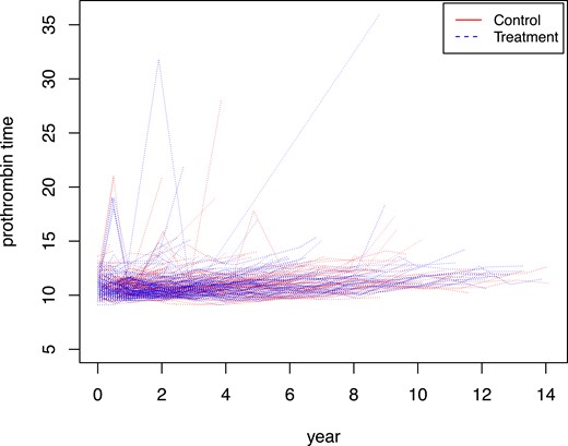
In this subsection, we apply the proposed -based tests to two real data sets. PBC data: The first data set is the PBC data from Mayo Clinic (Fleming & Harrington, 2005). This data set is from a clinical trial studying PBC of the liver. There were 312 patients assigned to either the treatment or control group. The drug D-penicillamine is given to the treatment group. Here, we are interested in testing the equality of the marginal distributions of prothrombin time, which is a blood test that measures how long it takes blood to clot. The trajectories of prothrombin time for different subjects are plotted in Figure 2, and there are on average six measurements per subject. For our tests, the bandwidth is set to be 2. Here, the equal distribution assumption for errors seems to work (the estimated variances for treatment and control group are 0.96 and 1.009, respectively). By using 200 permutations, the p-value of the -based test is 0.54, which means that there is not enough evidence to conclude that the marginal distributions of prothrombin time are different between the two groups. This conclusion matches with existing knowledge that D-penicillamine is ineffective to treat PBC of liver.
Trajectories of real data.
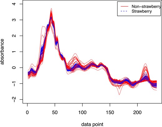
Strawberry data: In the food industry, there is a continuing interest in distinguishing the pure fruit purees from the adulterated ones (Holland et al., 1998). One practical way to detect adulteration is by looking at the spectra of the fruit purees. Here, we are interested in testing the marginal distribution between the spectra of strawberry purees (authentic samples) and non-strawberry purees (adulterated strawberries and other fruits). The strawberry data can be downloaded from the UCR Time Series Classification Archive (Dau et al., 2018; https://www.cs.ucr.edu/˜eamonn/time_series_data_2018/). The single-beam spectra of the purees were normalized to back-ground spectra of water and then transformed into absorbance units. The spectral range was truncated to 899–1802 (235 data points). The two samples of spectra are plotted in Figure 2 and more information about this data set can be found at Holland et al. (1998). The estimated variances of the measurement errors are 0.000279 and 0.00031 for the two samples, which indicates that there are practically no measurement errors. To check the performance of our method, we analyse the data using all 235 measurements as well as sparse subsamples that contain 2–10 observations per subject. The R package ‘energy’ is applied for the complete data. Both tests are conducted with 200 permutations and have p-value 0.005. Thus, we have strong evidence to conclude that the marginal distributions between the spectra of strawberry and non-strawberry purees are significantly different and our test produced similar results regardless of the sampling plan.
4 Conclusion
The literature on testing homogeneity for functional data is scarce probably because most approaches rely on intensive measurement schedules and the hope that measurement errors could be addressed by presmoothing the data. Since reconstruction of noise-free functional data is not feasible for sparsely observed functional data, a test of homogeneity is infeasible. In this work, we show what is feasible for sparse functional data, a.k.a. longitudinal data, and propose a test of marginal homogeneity that adapts to the sampling plan and provides the corresponding convergence rate. Our test is based on ED with a focus on testing the marginal homogeneity. To the best of our knowledge, this is the only nonparametric test with theoretical guarantees under sparse designs, which are ubiquitous.
There are several twists in our approach, including the handling of asynchronized longitudinal data and the unconventional way that measurement errors affect the method and theory. The asynchronization of the data can be overcome completely as we demonstrated in Section 2.1, but the handling of measurement errors requires some compromise when the distributions of the measurement errors are different for the two samples. This is the price one pays for lack of data and is not due to the use of the norm associated with testing the marginal homogeneity, as an norm for testing full homogeneity would also face the same challenge with measurement errors unless a presmoothing step has been employed to eliminate the measurement errors. As we mentioned in Section 1, this would require a super intensive sampling plan well beyond the usual requirement for dense or ultra-dense functional data (Zhang & Wang, 2016). While the new approach may involve error augmentation, numerical results show that the efficiency loss is minimal. Moreover, such an augmentation strategy is not uncommon. For instance, an error augmentation method has also been adopted in the SIMEX approach (Cook & Stefanski, 1994) to deal with measurement errors for vector data.
While testing marginal homogeneity has its own merits and advantages over a full-fledged test of homogeneity, our intention is not to particularly endorse it. Rather, we point out what is feasible and infeasible for sparsely or intensively measured functional data and develop theoretical support for the proposed test. To the best of our knowledge, we are the first to provide the convergence rate for the permuted statistics for sparse functional data. This proof and the proof of consistency for the proposed permutation test are non-conventional and different from the multivariate/high-dimensional case.
5 Technical details
5.1 Proof of Theorem 1
Here, we show that
and can be bounded similarly. For , set
where ; otherwise . The weighted raw data are denoted as
If there is no confusion, we will only write , instead of , for simplicity. Both (5) and (6) admit closed form solutions and some algebra show that for
Here, are two-dimensional functions defined as
where for , have the following expressions:
By some straight-forward calculations, for
where for ,
and
Lemma 3 entails that the denominator in (13) is bounded away from 0 with high probability. Thus, for , we have
It can be easily seen that if , and if . By Taylor expansion
where
5.2 Proof of Theorem 2
For any permutation π, let be the estimated function based on the permuted sample
Correspondingly, the explicit form of depends on the following quantities:
For , let be defined similarly with with replaced by , respectively. Then it can be shown that admits a similar form as with replaced by , .
The following lemma shows that as well as converge to their mean functions, where Π is a random permutation sampled uniformly from .
Under the assumptions of Theorem 2, for any , we have
- for any fixed permutation ,where C is a constant that depends on . Moreover, satisfies the same bound.
- For any random permutation Π sampled from uniformly,where C is a constant that depends on . Moreover, can attain the same rate as above.
Under the assumptions of Theorem 2, for any , we have
- for any fixed permutation ,
- For any random permutation Π sampled from uniformly,
(ii) The result follows from the fact that the upper bounds in (17) and (18) hold uniformly for all permutations in . □
Next, we resume the proof of Theorem 2. For any , we set
By symmetry of the kernel K, if or . Consequently, by Lemmas 2 and 3, if ,
Otherwise, would converge to a positive constant in probability. This also implies that the denominator of is bounded away from 0 with high probability. Thus,
which entails that
5.3 Proof of Theorem 3
Under , set . By Theorems 1 and 2,
5.4 Proof of Corollary 2
Under Assumptions 1, 2, and 4, the result can be shown by adopting similar arguments as in the proof of Theorem 1 by replacing , , , , with , , , , , respectively.
5.5 Proof of Theorem 4
5.6 Proof of Corollary 3
Funding
This research was supported by NIH grant UH3OD023313 (ECHO programme) and NSF DMS-2210891 and DMS-1914917.
Data availability
The data are available in the book ‘Counting Process and Survival Analysis’ by Thomas R. Fleming and David P. Harrington (2005) [https://onlinelibrary.wiley.com/doi/book/10.1002/9781118150672] and from the UCR Time Series Classification Archive [https://www.cs.ucr.edu/eamonn/time_series_data_2018/].
References
Author notes
Conflict of interest: We have no conflicts of interest to disclose.
